Unsupervised Cross-Domain Soft Sensor Modelling via Deep Physics-Inspired Particle Flow Bayes
Abstract
Data-driven soft sensors are essential for achieving accurate perception through reliable state inference. However, developing representative soft sensor models is challenged by issues such as missing labels, domain adaptability, and temporal coherence in data. To address these challenges, we propose a deep Particle Flow Bayes (DPFB) framework for cross-domain soft sensor modeling in the absence of target state labels. In particular, a sequential Bayes objective is first formulated to perform the maximum likelihood estimation underlying the cross-domain soft sensing problem. At the core of the framework, we incorporate a physics-inspired particle flow that optimizes the sequential Bayes objective to perform an exact Bayes update of the model extracted latent and hidden features. As a result, these contributions enable the proposed framework to learn a rich approximate posterior feature representation capable of characterizing complex cross-domain system dynamics and performing effective time series unsupervised domain adaptation (UDA). Finally, we validate the framework on a complex industrial multiphase flow process system with complex dynamics and multiple operating conditions. The results demonstrate that the DPFB framework achieves superior cross-domain soft sensing performance, outperforming state-of-the-art deep UDA and normalizing flow approaches.
Index Terms:
Bayesian deep learning, soft sensor, domain adaptation, unsupervised learning, particle filtering.I Introduction
Rapid evolution of industrial instrumentation, computing, and communication in recent years have fueled a growing demand for complex systems with rich dynamics. Accurate estimation of both the representations of the dynamic system and its operating condition is often critical for monitoring and control. These system representations often consist of a set of mutually exclusive state variables that encapsulate the information needed to describe the system’s behavior over time. In this context, inference models such as soft sensors and discrete filters play a crucial role in predicting these states (labels), given the time series measurements (data) from the integrated physical sensors.
Following the rise of deep learning, neural networks (NNs) have been widely adopted as soft sensors in both autonomous systems and industrial processes [1]. However, most deep learning-based soft sensor models assume that training and testing data are drawn from a single domain with a unified distribution [2]. This assumption is highly unrealistic in practice, as industrial systems and processes exhibit distinct dynamics and data distributions under different operating conditions [3]. Consequently, deep soft sensor models trained on data collected from preset conditions (source domains) cannot generalize well to target applications with unseen operating conditions (target domains). Although the soft sensor models could be rebuilt using data and labels collected from the target domains, it is inefficient. Moreover, obtaining state labels in many industrial systems is not as straightforward as acquiring measurement data, readily provided by the physical sensors. In many circumstances, collecting representative labels on target operating conditions may be too expensive or unattainable [4], ultimately leading to missing labels in the target domains.
To tackle the challenge of distributional mismatch between domains and the problem of missing labels, unsupervised domain adaptation (UDA) has shown immense potential in leveraging unlabelled target data to generalize deep learning models beyond the labelled source data [5]. A plethora of feature-based deep UDA models have been proposed for cross-domain time series data analysis in many important applications [6]. These UDA models predominantly rely on deep domain adaptation techniques such as stacked autoencoders (AEs) [7, 8, 9, 10], domain adversarial training (DAT) [11, 12, 13, 14], variational Bayes (VB) [15, 16, 17, 18] to extract nonlinear domain-invariant feature representations that can be adapted to both source and target domains. Recently, deep probabilistic UDA models [19, 20, 21, 22] that combine the auto-encoding variational Bayes (AEVB) framework [23] with DAT have seen improved robustness to incomplete data via better predictive uncertainty quantification. Due to the intrinsic capacity of the AEVB framework in characterizing stochastic data, these models provide a probabilistic data modelling solution ideal for dynamic industrial systems [24].
Despite the widespread success of existing deep UDA models, several major issues remain. To address covariate shift, these models rely on the domain invariance assumption, which assumes that the posterior distribution of features remains the same across the source and target domains. However, this assumption compromises the expressive power of the resulting feature representation [17]. Additionally, the AEVB framework implements the variational approximation, which employs a mean-field parametric posterior distribution with highly localized density and limited generalization capability [25]. The drawbacks, when combined, could impede effective domain adaptation and result in a inadequate characterization of the complex cross-domain time series data. Secondly, deep UDA models are typically trained using exclusive source and target time series data, which is challenging to collect from specific domains in many industrial systems due to their perpetually varying operating conditions. Moreover, these domain-specific data overlook the complex dynamics that occur during transitions between domains. Therefore, to address the unsupervised cross-domain soft sensing problem, it is crucial to develop end-to-end models that can perform UDA on time series data consisting of switching domains, which has not been extensively studied in the literature [21]. Finally, while RNNs are capable of capturing complex temporal dependencies and factors of variation underlying time series data [26], existing RNN-based UDA models do not subject these hidden states to domain adaptation. As a consequence, this could preclude the extensive adaptation of temporal coherence across time series from distinct domains [19].
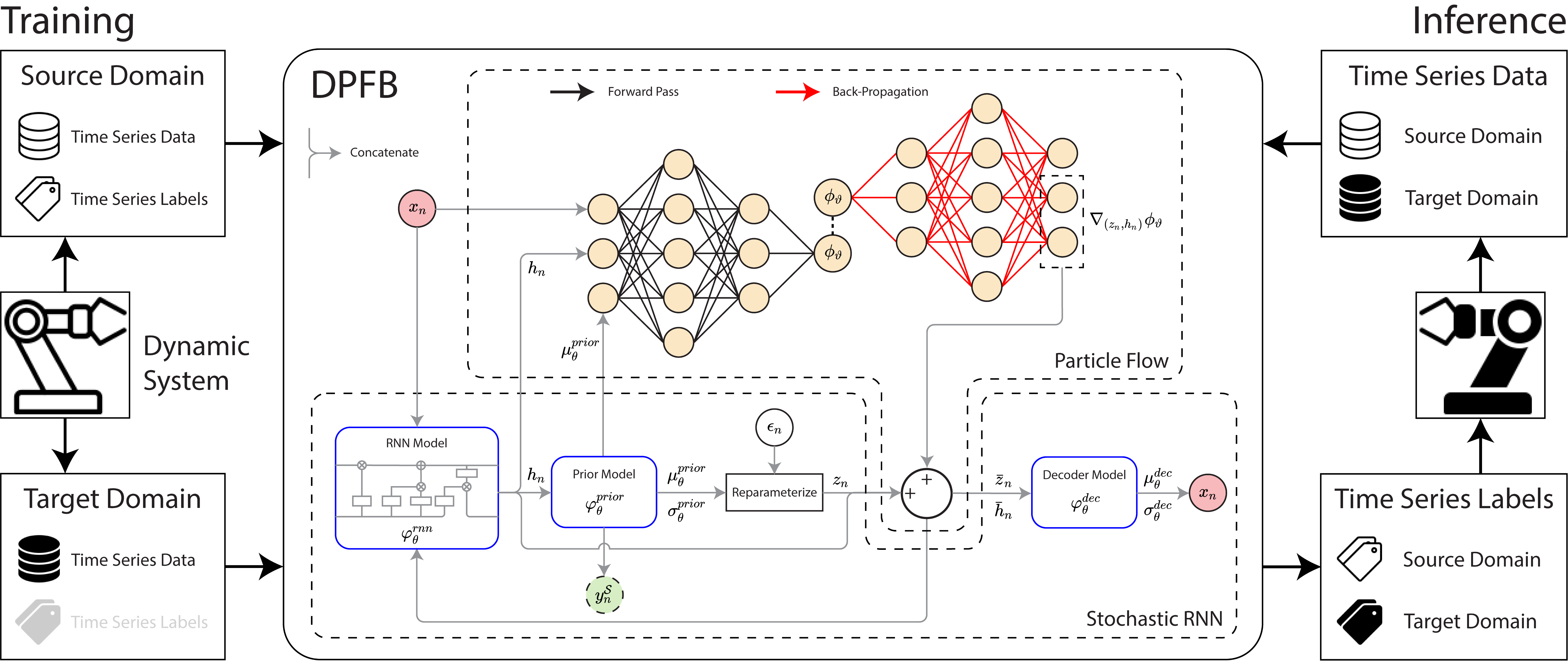
In this paper, we propose a deep Particle Flow Bayes (DPFB) framework to address the unsupervised cross-domain soft sensing problem in dynamic systems with varying operating conditions. The DPFB framework learns a cohesive approximate posterior feature representation that accurately characterizes the complex cross-domain system dynamics, thereby facilitating effective unsupervised time series domain adaptation. In addition, our proposed framework abstains from the restrictive domain invariance assumption and variational approximation in retaining the domain-adaptability and nonlinear data modelling capability of the learned feature representation. Fig. 1 provides an overview of the proposed framework. To the best of knowledge, this is the first work that investigates deep particle flow for cross-domain soft sensor modelling. Our contributions are highlighted as follows:
-
•
A sequential Bayes objective is formulated to perform maximum likelihood estimation of the cross-domain time series data and source labels. This objective underpins the proposed framework and inherently facilitates a Bayes update of the model extracted latent and hidden features.
-
•
A physics-inspired particle flow that resembles the advection of fluid in a potential-generated velocity field, is proposed to transport the model extracted feature samples. A flow objective is derived to enable the particle flow in performing a Bayes update to endow the transported features with a representative approximate posterior.
-
•
The proposed DPFB framework is validated on a real industrial system with complex dynamics and multiple operating conditions. Benchmark results show that amidst the missing target labels, DPFB achieves superior cross-domain soft sensing performances in comparison to state-of-the-art deep UDA and normalizing flow approaches.
The rest of the paper is organized as follows: Section II outlines the backgrounds of time series UDA and sequential AEVB. Section III details the formulation of our proposed DPFB framework. A real industrial case study is presented and discussed in Section IV. Section V concludes the paper.
II Backgrounds
II-A Unsupervised Time Series Domain Adaptation
UDA is a special case of transfer learning, where the source and target domains are from the same space and the labels are missing in the target domain [6]. Consider a sequence of data and label subspace pairs and of length , known respectively as the source and target domains with distinctive marginal data distributions . The objective of time series UDA is to predict the missing target labels , using the cross-domain data and source labels [5]. In general, deep UDA models achieve this by learning, at each sample index , a domain-invariant latent feature space that generalizes well across domains, so that it accurately predicts the labels in both the label spaces . On one hand, the DAT-based models [11, 12, 13, 14] incorporate a feature-level domain discriminator, where its adversarial gradients are backpropagated to train the feature extractors in generating domain-invariant feature representations. On the other hand, the VB-based models [15, 16, 17, 18] implement variational inference to learn domain-invariant probabilistic latent feature representations that generalize the knowledge learned from the supervised source domain to the unsupervised target domain. Nevertheless, these deep UDA approaches hinge on the assumption of domain invariance, which could impede the generalization and expressive abilities of feature models in characterizing complex cross-domain system dynamics [27].
II-B Sequential Auto-Encoding Variational Bayes
The AEVB is a class of probabilistic deep learning framework that aims to maximize the lower bound of the joint data log-likelihood . By introducing a latent state , a variational evidence lower bound (ELBO) of the data log-likelihood can be obtained via the importance decomposition , where denotes the (positive-valued) Kullback-Leibler divergence (KLD). The data likelihood , the latent approximate posterior distribution , and the latent prior distribution are mean-field Gaussians parameterized respectively by the fully-connected neural network (FCNN) models: decoder, prior, encoder, known collectively as the variational AE (VAE). The parameters and denote the set of NN parameters governing these models. A significant drawback of VAE is the assumption that the time series data are independent and identically distributed (i.i.d.), which falls short at capturing the underlying temporal characterization. To address this, the sequential AEVB framework [28] introduces a sequential ELBO as follows:
| (1) | ||||
where denotes a partial sequence up to the sample. Similarly, the conditional data likelihood , the latent prior distribution , and the approximate posterior are mean-field Gaussians parameterized by RNN models, known collectively as the variational RNN (VRNN). However, existing VRNN-based approach rely on the variational approximation, which significantly compromises their generalization capability to perform effective domain adaptation. Moreover, the RNN hidden states are not explicitly subjected to posterior update, which could result in poorly conditioned hidden states that generate latent features divergent from the actual system representation.
II-C Particle Flow
Bayesian inference, which is a more general approach than variational inference [29], constructs an exact approximation of the true posterior recursively via the Bayes rule . Particle flow, first introduced in [30], achieves this by subjecting prior samples to a series of infinitesimal transformations that follow a linear ordinary differential equation (ODE) in continuous pseudo-time . The function , known as the velocity, is formulated such that the flow inherently performs the Bayes update, and the transformed samples represent an empirical (Monte Carlo) approximation of the true posterior. While particle flow is closely related to normalizing flows [31, 25] for variational inference, the latter do not exhibit a Bayes update. Pal et al. [32] recently combined graph representation learning with particle flow for spatiotemporal time series forecasting, but relied on restrictive local linearization for nonlinear models. Nonetheless, existing flow-based methods do not consider the issues of domain shift and missing labels.
III Methods
In this section, we develop the deep Particle Flow Bayes (DPFB) framework. First, we consider the cross-domain time series maximum likelihood problem, which results in a sequential Bayes objective (SBO). Then, a RNN-based parameterization is introduced for the SBO to sample stochastic temporal features. Finally, we propose a physics-inspired particle flow that performs exact Bayes update of the extracted features.
III-A Semi-supervised Sequential Bayes Objective
From a probabilistic perspective, the unsupervised cross-domain soft sensor modelling problem can be viewed as maximizing the joint likelihood of the cross-domain time series data and the source labels. The maximum likelihood problem can be formulated as follows:
| (2) | ||||
Taking into account the difficulty of directly optimizing (2), we introduce a sequence of stochastic latent state space and consider an importance decomposition of the conditional data log-likelihood that holds for any choice of approximate posterior as follows:
| (3) | ||||
where
| (4) | ||||
Here, denotes the intractable true joint latent posterior . Also, we assumed that , i.e., the true posterior is self-sufficient and gains no further information from observing the labels.
Subsequently, we consider factorizing the conditional data likelihood in (3) as follows:
| (5) | ||||
where we assumed that , i.e., the approximate posterior latent sequence accurately characterizes the preceding time series . Finally, substituting (5) into (3), we obtain the sequential Bayes objective (SBO) as follows:
| (6) | ||||
As a result, we reformulated the cross-domain soft sensing problem as an end-to-end expectation-maximization algorithm (6). In the maximization step, the first two objectives identify a pair of generative data likelihood and label likelihood that represent the cross-domain data and source labels. In the expectation step, the last two objectives aim to find the optimal marginal approximate posterior and joint approximate posterior that resemble the conditional prior and the intractable true posterior , respectively.
In particular, the first three objectives in (6) are the same as those in the VRNN’s sequential ELBO (1). However, we have added an additional (third) semi-supervised objective to account for the source labels. In addition to these objectives, our SBO formulation includes the final KLD objective, which inherently performs a Bayesian smoothing [29] of the partial state sequence . This Bayesian smoothing encourages the latent state sequence to adopt an approximate posterior feature representation that facilitates a comprehensive characterization of the cross-domain time series data.
III-B Recurrent Neural Network Parameterization
In this subsection, we introduce a RNN parameterization for the proposed SBO. First, we parameterize the generative data and label likelihoods, and the latent prior in (6) as Gaussian distributions, given by:
| (7a) | ||||
| (7b) | ||||
| (7c) | ||||
where and are isotropic covariances, and denotes the diagonal function. In particular, we allow the latent prior (7c) to coincide with the label likelihood (7b), allowing the models to learn to predict the source labels. This supervised knowledge in the source domain can then be adapted to the unsupervised target domain during the Bayes update of the proposed particle flow.
Subsequently, the mean and standard deviation pairs in (7) are obtained using a stochastic RNN as follows:
| (8a) | ||||
| (8b) | ||||
| (8c) | ||||
where is the RNN model, and the prior model , decoder model and state encoding model are FCNNs. Here, the memory-encoding RNN hidden states serve as an embedding of the preceding time series to retain the intrinsic temporal information; this allows us to work with a reduced-dimension state space instead of the exponentially growing for the entire latent sequence, thus avoiding curse of dimensionality [33].
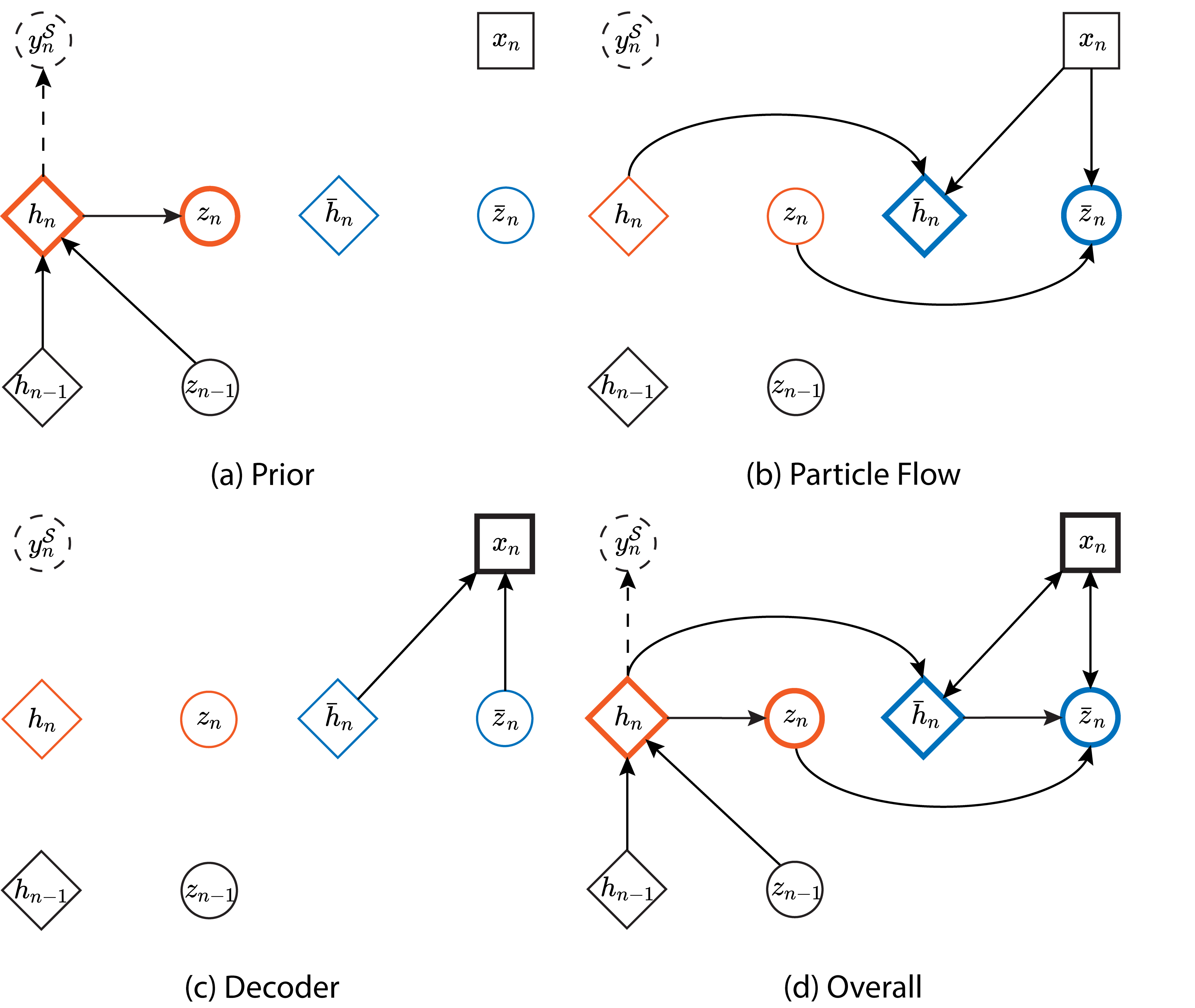
To sample from the latent prior , we compute its mean and standard deviation using equations (8a) to (8b), and then apply the reparameterization trick [23]. It is worth noting that although the hidden states have a degenerate conditional distribution , where is the Dirac delta function, they remain stochastic due to the recurrence and the variability of latent states after integrating out the conditioned variables. Additionally, unlike in VRNN [28], data are not fed into the RNN model to minimize the inheritance of data noise. Fig. 2 outlines the (features) prior and (data) decoder operations in DPFB.
III-C Particle Flow for Bayesian Inference
In this subsection, we introduce particle flow as a Bayesian inference technique to parameterize the approximate posterior. More precisely, a set of sampled prior latent and hidden state particles is subjected to a series of infinitesimal transformations, collectively mapping them to . These FCNN-parameterized transformations, denoted individually as , are governed by an ODE on a continuous pseudo-time interval . The flow velocity function is designed to induce a Bayes update, such that the transformed particles empirically constitute an approximate posterior that statistically resembles the true posterior .
In particular, we sample the prior particles using the RNN and prior models (8a)-(8b), given transformed particles from the previous sample. Incorporating the RNN parameterization (8) followed by the particle flow into our SBO (6), we obtain
| (9) | ||||
where we obtain the third objective using the density transformation . Here, denotes the determinant operator, and denotes the Jacobian of with respect to its input variables.
Integrating particle flow into our framework provides two key advantages. First, it results in an end-to-end learning framework that eliminates the disjointed encoder model in VRNN. This prevents unstable KLD gradients that arises from divergent prior and encoder distributions [34]. Second and more importantly, it preserves the expressive and generalization powers of the approximate posterior by overcoming the restrictive variational approximation. Nevertheless, it is not possible to directly optimize the KLD in (9) due to the intractable true posterior . Taking this into account, we propose the particle flow in the following section.
III-D Deep Physics-Inspired Particle Flow
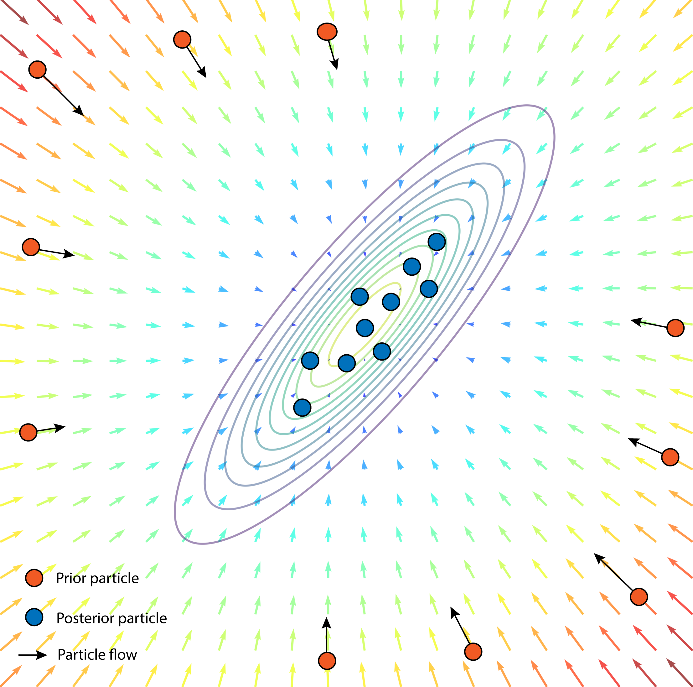
In this subsection, we propose a physics-inspired particle flow that draws inspiration from the control-oriented approaches [35, 36] to Bayesian inference. The proposed particle flow simulates fluid advection, where the flow (transport) of fluid is driven by an irrotational potential-generated velocity field. We provide a planar illustration of the particle flow in Fig. 3. Subsequently, we derive a tractable flow objective that solves the minimum KLD problem in the SBO (9). Consequently, the particle flow learns to inherently perform a Bayes update on the RNN-extracted features towards constructing a representative approximate posterior.
Our proposed particle flow takes the following form:
| (10) |
where denotes the Del operator (gradient) with respect to . Here, we parameterize the normalized (mean-subtracted) velocity potential as FCNN. By discretizing (10) using a forward Euler scheme with step size , we obtain the infinitesimal piecewise-linear transformation given by:
| (11) | ||||
Here, represent the trajectories traced out by the feature particles, as they undergo the particle flow over the defined pseudo-time interval . Therefore, the particle trajectories begin at the initial coordinates and end at final coordinates .
As a direct consequence, the proposed particle flow (10) induces an evolution in the resulting empirical distribution , which can be described by a Kolmogorov forward equation as follows:
| (12) |
where denotes the divergence operator . Upon closer examination, it becomes apparent that this forward equation is in fact a continuity equation which governs the advection of fluid, uncovering its fundamental connection to physics. In particular, corresponds to the fluid density, and represents the driving velocity potential. The resulting gradient acts as the irrotational (conservative) velocity field, as illustrated by the (coloured) arrows in Fig. 3.
Next, we derive a tractable flow objective for the proposed particle flow (10)-(11) using the calculus of variations in two stages, so that it induce a Bayes update of the RNN-extracted prior feature particles. In the first stage, Proposition 1 shows that solving the minimum KLD problem is equivalent to solving a partial differential equation (PDE). In the second stage, Proposition 2 yields a tractable particle flow objective that provides a weak solution to the aforementioned PDE.
Proposition 1.
Assuming the following hold:
-
1.
The prior distribution (before particle flow) has compact support on .
-
2.
The preceding approximate posterior (after particle flow) is a good approximation to the true posterior .
-
3.
The pseudo-time step size is sufficiently small.
Considering a particle flow of the form (10), the problem of minimizing the KLD in (9):
| (13) | ||||
is then equivalent to finding the velocity potential that satisfies the following PDE:
| (14) | ||||
where denotes the normalized innovation squared (NIS):
| (15) | ||||
and denotes its mean .
Proof.
Refer to Supplementary Materials. ∎
Proposition 2.
The following particle flow objective:
| (16) | ||||
is equivalent to solving the weak formulation of PDE (LABEL:eq:Proposition_1_PDE), given that . Here, denotes the Euclidean norm, denotes the covariance, and denotes the Sobolev space of square-integrable scalar functions whose first derivative is also square-integrable.
Proof.
Refer to Supplementary Materials. ∎
Remark.
The second assumption of Proposition 1 becomes more accurate as training progresses. The velocity potential are modelled as FCNN (with leaky ReLU activation), which is shown to be universal approximator in Sobolev spaces [37].
To summarize, Propositions 1 and 2 have allowed us to reformulate the intractable minimum KLD problem (13) as a tractable particle flow objective (16). As a result, by optimizing the velocity potential with respect to (16) and transporting the prior samples through the corresponding infinitesimal transformations (11), we are able to perform exact, non-variational Bayesian update of the RNN-extracted feature particles to obtain an empirical approximate posterior that accurately resembles the true posterior in a statistical sense.
The minimum covariance objective in (16) plays a crucial role as it ensures that a decrease in the NIS (15) corresponds to an increase in the velocity potential. The gradient consistently points in the direction of greatest potential ascent, and by minimizing the covariance, we guarantee that the potential-generated velocity field drives the flow of latent particles towards the high probability regions of true posterior distribution, as illustrated in Fig. 3. These regions, characterized by low NIS values, are where the true posterior is concentrated. As a result, the proposed particle flow inherently performs a Bayes update of the RNN-extracted features to facilitate effective learning and adaptation.
Given that the sampling rate is high enough to accurately represent the underlying system dynamics with negligible sampling error, we can set and perform the particle flow (10)-(11) in a single step. Additionally, to improve data characterization in the velocity potential, we incorporate a measurement encoding FCNN model to extract useful features from the data. After incorporating these considerations and replacing the minimum KLD problem in (9) with the particle flow objective (16), the final SBO for our DPFB framework is given by:
| (17) | ||||
Here, we opted to exclude the third objective in (9) for our implementation to avoid the computation of the expensive Jacobian determinant term.
On that note, we conclude the development of our proposed DPFB framework. Overall, the framework intrinsically performs an end-to-end expectation-maximization algorithm. In the maximization step, the stochastic RNN learns to model a generative (features) prior and a (data) decoder likelihood that captures the distributional uncertainties of the cross-domain data and source labels. Using the pair of feature prior and data likelihood, the expectation step construct a cohesive approximate (features) posterior that is representative of the unsupervised data across domains. These steps performed together, allow the framework to learn a domain-adaptive probabilistic feature representation that accurately characterizes complex cross-domain system dynamics and effectively facilitates cross-domain soft sensor modelling. Fig. 2 outlines the particle flow operation in DPFB, where it bridges the (features) prior and the (data) decoder.
| Flow rate of input air (m3/s) | 0.0208 | 0.0278 | 0.0347 | 0.0417 | |
|---|---|---|---|---|---|
| Flow rate of input water (kg/s) | 0.5 | 1 | 2 | 3.5 | 6 |
IV Case Study
In this section, we present an industrial case study using a complex multivariate time series dataset collected from a real industrial-scale multiphase flow (MFP) system. The multiple operating conditions and complex dynamics of this MFP system make it a suitable candidate for evaluating the efficacy of deep UDA methods in cross-domain soft sensing.
| Type | No. | Location | Variable description | Unit |
|---|---|---|---|---|
| Data | 1 | LI405 | Level of two-phase separator | m |
| 2 | FT104 | Density in water input | kg/m3 | |
| 3 | LI504 | Level of three-phase separator | % | |
| 4 | VC501 | Position of valve VC501 | % | |
| 5 | VC302 | Position of valve VC302 | % | |
| 6 | VC101 | Position of valve VC101 | % | |
| 7 | PO1 | Water pump current | A | |
| State Labels | 1 | PT312 | Pressure of input air | MPa |
| 2 | PT401 | Pressure in bottom of the riser | MPa | |
| 3 | PT408 | Pressure in top of the riser | MPa | |
| 4 | PT403 | Pressure in two-phase separator | MPa | |
| 5 | PT501 | Pressure in three-phase separator | MPa | |
| 6 | PT408 | Differential pressure (PT401-PT408) | MPa | |
| 7 | PT403 | Differential pressure (over VC404) | MPa | |
| 8 | FT305 | Flow rate of input air | m3/s | |
| 9 | FT104 | Flow rate of input water | kg/s | |
| 10 | FT407 | Flow rate in top of the riser | kg/s | |
| 11 | FT406 | Flow rate of two-phase separator output | kg/s | |
| 12 | FT407 | Density in top of the riser | kg/m3 | |
| 13 | FT406 | Density of three-phase separator output | kg/m3 |
IV-A Systems Description
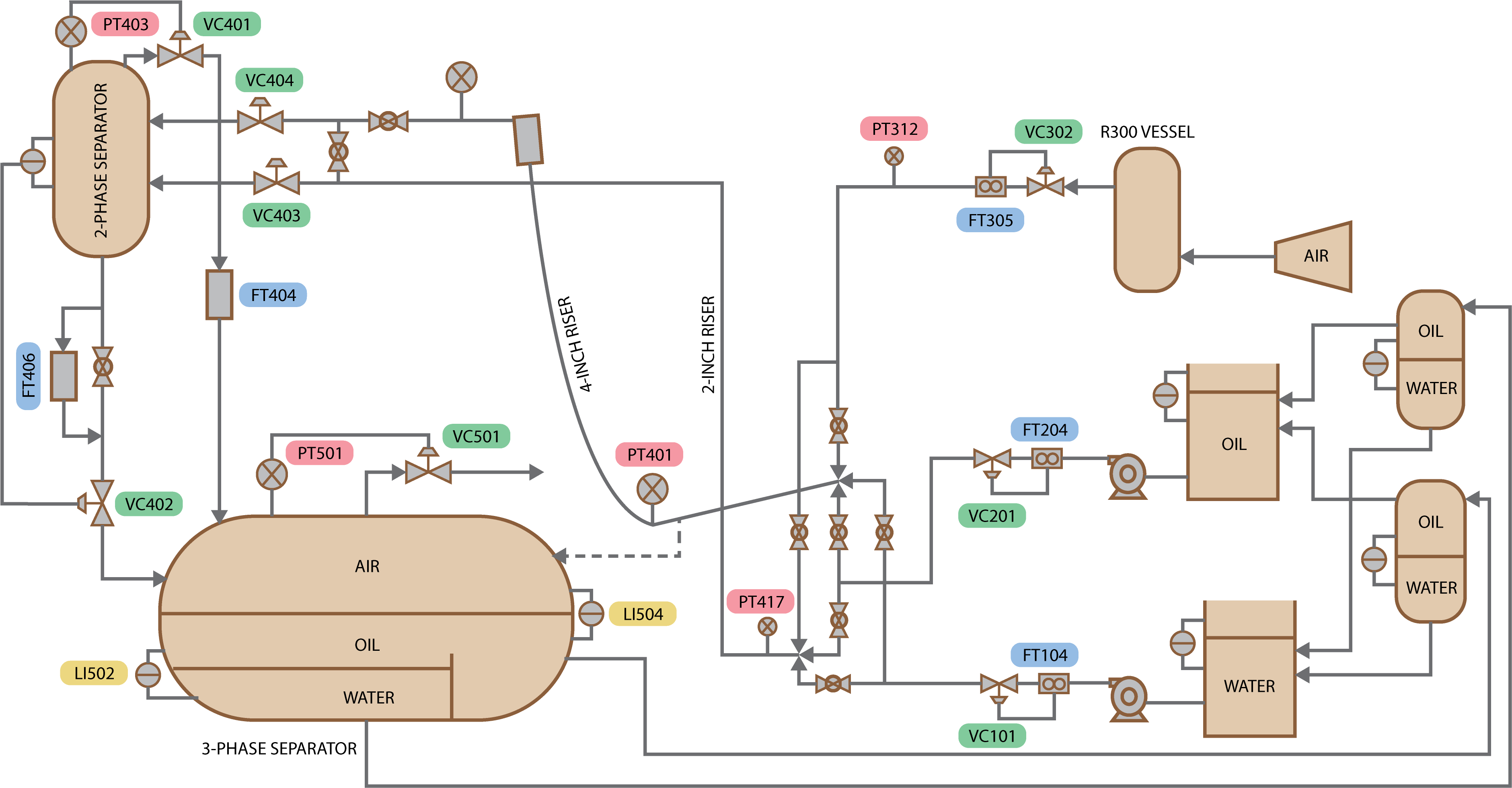
The Cranfield Multiphase Flow Process (MFP) [38] is a real industrial process that employs advanced condition monitoring techniques based on heterogeneous sources. The Cranfield MFP is designed to provide a controlled and measured flow rate of water, oil, and air to a pressurized system. The process flow diagram is illustrated in Fig. 4, and a detailed description of the process can be found in [38].
During the data collection process, the air and water flow rates were deliberately varied between the set points (operating conditions) listed in Table I to obtain a good variety of process changes and capture a wide range of distinct dynamics. For this case study, the variables that require specialized measurement sensors, including pressure, flow rate, and density, are identified as the states that need to be predicted using the proposed soft sensor model. The remaining variables are considered as measurement data, which the model utilizes for state prediction. Table II provides a list of all MFP variables. All variables are sampled at 1 Hz.
IV-B Benchmarking
To evaluate the cross-domain soft sensing performance of our proposed framework, we compare it against several state-of-the-art UDA approaches based on deep autoencoder: DLSN [7], domain adversarial: DARNN [11], variational Bayes: MVI [15] and a combination of these concepts: VRADA [19], InfoVDANN [20] and DPTR [21]. Note that we have extended DSLN and MVI based on their respective sequential counterparts [39, 40] to allow for time series regression. The RNNs in these baseline approaches are designed to be single-layered Long Short-Term Memory (LSTM) networks for capturing complex temporal patterns. Additionally, we include a stacked (three-layered) LSTM [26] trained on complete source and target labels (termed LSTM-C) to benchmark the overall UDA performances. Furthermore, to outline the importance of the physic-inspired particle flow in our proposed framework, we replace it with two widely recognized normalizing flows: IAF [31] and iResNet [41]. To demonstrate the resilience of the proposed framework to particle degeneracy, we also compare it with a deep probabilistic model based on particle filtering: FIVO [42]. All these baselines are trained with missing target labels, and their architectures are designed to match the number of model parameters in DPFB.
IV-C Experimental Setup
The MFP dataset contains three data sequences with 13200, 10372 and 9825 data points, respectively. The first two are used for training and the last one is used for testing. The target (state) labels in the testing dataset serve only as ground-truths for result validation. For the purpose of unsupervised domain adaptation, the data region in which the air flow rate variables range from 0.0278 - 0.0347 m3/s is considered as the source domain, which constitutes 45% of the entire training data. The region where the air flow rate is outside of this range is considered as the target domain, where the state labels are assumed to be missing. Taking into account the conditions, the time series data (and labels) consist of time windows that switch between the two domains, as shown in Fig. 5.
| Variable | Pressure (State Labels No. 1-7) | Flow Rate and Density (State Labels No. 8-13) | ||||||||||
|---|---|---|---|---|---|---|---|---|---|---|---|---|
| Method | Prediction Error (NRMSE) | Coefficient of Determination (R) | Prediction Error (NRMSE) | Coefficient of Determination (R) | ||||||||
| Source | Target | Overall | Source | Target | Overall | Source | Target | Overall | Source | Target | Overall | |
| LSTM-C [26] | 0.395±0.015 | 0.403±0.018 | 0.400±0.016 | 0.707±0.023 | 0.736±0.015 | 0.726±0.017 | 0.249±0.014 | 0.306±0.016 | 0.281±0.014 | 0.844±0.018 | 0.860±0.015 | 0.866±0.015 |
| DLSN [7] | 0.527±0.019 | 0.594±0.021 | 0.567±0.018 | 0.594±0.024 | 0.512±0.039 | 0.549±0.030 | 0.342±0.017 | 0.496±0.009 | 0.434±0.010 | 0.769±0.023 | 0.729±0.019 | 0.757±0.016 |
| DARNN [11] | 0.501±0.045 | 0.659±0.047 | 0.592±0.030 | 0.530±0.096 | 0.405±0.099 | 0.469±0.070 | 0.300±0.020 | 0.652±0.018 | 0.522±0.009 | 0.797±0.038 | 0.559±0.019 | 0.653±0.006 |
| MVI [15] | 0.586±0.007 | 0.612±0.022 | 0.600±0.009 | 0.332±0.003 | 0.432±0.042 | 0.399±0.025 | 0.274±0.008 | 0.496±0.020 | 0.407±0.015 | 0.826±0.005 | 0.703±0.021 | 0.761±0.013 |
| VRADA [19] | 0.467±0.012 | 0.558±0.016 | 0.494±0.007 | 0.592±0.041 | 0.552±0.024 | 0.580±0.016 | 0.260±0.011 | 0.558±0.008 | 0.494±0.009 | 0.832±0.012 | 0.612±0.012 | 0.684±0.013 |
| InfoVDANN [20] | 0.616±0.022 | 0.610±0.006 | 0.613±0.014 | 0.284±0.045 | 0.447±0.012 | 0.390±0.025 | 0.296±0.010 | 0.518±0.030 | 0.428±0.022 | 0.803±0.006 | 0.695±0.018 | 0.748±0.013 |
| DPTR [21] | 0.559±0.005 | 0.663±0.010 | 0.617±0.008 | 0.391±0.026 | 0.391±0.008 | 0.406±0.013 | 0.326±0.010 | 0.657±0.027 | 0.529±0.021 | 0.748±0.005 | 0.561±0.048 | 0.650±0.026 |
| IAF [31] | 0.492±0.036 | 0.672±0.045 | 0.594±0.023 | 0.527±0.085 | 0.356±0.086 | 0.440±0.058 | 0.259±0.015 | 0.538±0.016 | 0.433±0.015 | 0.823±0.016 | 0.653±0.009 | 0.725±0.008 |
| iResNet [41] | 0.484±0.045 | 0.679±0.047 | 0.596±0.046 | 0.543±0.132 | 0.370±0.089 | 0.460±0.097 | 0.256±0.010 | 0.606±0.023 | 0.475±0.016 | 0.829±0.003 | 0.592±0.013 | 0.692±0.009 |
| FIVO [42] | 0.703±0.036 | 0.752±0.028 | 0.730±0.030 | 0.169±0.086 | 0.194±0.080 | 0.193±0.080 | 0.374±0.024 | 0.637±0.022 | 0.532±0.022 | 0.727±0.019 | 0.548±0.014 | 0.629±0.016 |
| DPFB (ours) | 0.393±0.014 | 0.425±0.020 | 0.412±0.009 | 0.703±0.026 | 0.720±0.028 | 0.718±0.013 | 0.256±0.015 | 0.447±0.005 | 0.376±0.008 | 0.825±0.016 | 0.731±0.010 | 0.770±0.009 |
In terms of model architecture, our proposed DPFB framework employs a single-layered Gated Recurrent Unit (GRU) with a hidden state of size 512 as the RNN model . The prior model and the decoder model implemented as FCNNs with hidden layers {256, 128} and {512, 256, 128}, respectively. Here, each entry of the curly brackets is a hidden layer and the value denotes layer width. The state and measurement encoding model , are also implemented as FCNNs with hidden layers {256} and {128}, respectively. The velocity potential is modeled as a bottleneck FCNN with hidden layers {512, 256, 128}. These model hyperparameters are chosen based on training loss.
All proposed and baseline models are trained on batches of data and label sequences with a fixed length of 100. We optimize the models using the Adam optimizer with annealing and L2 regularization of 0.01, for 300 epochs. The batch sizes and initial learning rates are selected from 8, 16, 32 and 5, 1, 5, respectively. We use 8 sample particles during training, and a single particle without reparameterization during inference.
IV-D Results and Discussions
In this section, we evaluate the performances of DPFB and baselines using the metrics: State Prediction Error: the normalized root-mean-square error (NRMSE) between the predicted states and the ground-truth labels, to assess the accuracy of point state estimates based on the approximate posterior. Coefficient of Determination: the proportion of variation (R) between the predicted states and the ground-truths, to assess the unbiasedness and sharpness of the approximate posterior.
Table III shows the comparison results. Overall, our proposed DPFB outperforms the state-of-the-art VB and DAT methods, achieving the lowest state NRMSE and the highest R among the baselines. Furthermore, DPFB performs better with particle flow than the normalizing flows, IAF and i-ResNet, due to the Bayes update performed via the proposed physics-inspired particle flow. Unlike FIVO which attains low R2 scores due to repeated importance weighting and resampling, DPFB exhibits robustness to the particle degeneracy issue as it does not involve these particle filtering operations. Notably, the difference between the DPFB and the baselines grows larger on the unsupervised target domains consisting of unseen system dynamics. Moreover, the DPFB achieves scores that are closest to the fully-supervised LSTM-C benchmark. These results demonstrate the outstanding ability of DPFB in producing accurate state predictions amidst the missing target labels. Additionally, they show the DPFB’s capability to perform effective UDA on time series data with switching domains. By virtue of this capability, our framework addresses the cross-domain soft sensing problem in dynamic systems with varying operating conditions.
Fig. 5 shows the validation results of the state predictions against the ground truth labels. Notably, during the unsupervised time windows where the system operates in the target domains, the predictions of our proposed DPFB are able to track the ground truths more closely than the second-best performing VRADA. This is particularly evident in the air flow rate predictions in the third row of Fig. 5. Unlike VRADA, the air flow rate prediction of DPFB is not restricted within the predetermined source domain range of 0.0278 - 0.0347 m3/s. This capability of DPFB to generalize predictions beyond the source domains is due to its competence in accurately performing soft sensing (state inference) using unsupervised data. This is achieved through the proposed particle flow, which circumvents the variational approximation of variational Bayes and facilitates exact (non-variational) Bayesian inference of the state labels across both supervised and unsupervised domains.
Fig. 6 compares the PCA embeddings (using cosine kernel) of the extracted latent state features and the PCA embeddings of the ground truth labels. The latent state embeddings generated by our proposed DPFB model are found to be most consistent with the ground truth embeddings. Additionally, the PCA embeddings of the source and target domains exhibit less overlap in both the DPFB and ground truth embeddings compared to the other baseline methods. This can be attributed to the dispensing of domain-invariant enforcing techniques such as DAT in our DPFB framework, which helps in retaining the rich representation of the extracted posterior feature space. Consequently, the models can construct an inclusive joint (time) feature space capable of adopting complex cross-domain state representations of dynamic systems. These results illustrate the DPFB is more effective in generating accurate state predictions and constructing a cohesive probabilistic feature representation that better captures the underlying characteristics of the unsupervised data.
Fig. 7 presents the t-SNE embeddings of the extracted hidden state features from the RNN-based models. The hidden state embeddings of our proposed DPFB exhibit a structured temporal arrangement that closely resembles that of those of the fully-supervised LSTM-C benchmark. This similarity demonstrates the ability of the proposed particle flow to endow the RNN hidden states with temporal characteristics that are inherent the dynamic system. As a result, the endowed temporal coherence facilitates a smooth transition between the source and target time windows, enabling effective cross-domain soft sensor modelling. In contrast, baseline models that lack this temporal coherence experience difficulty in transitioning between the domains and leads to poor performance. These results highlight the importance of subjecting the hidden states to a Bayes update via the proposed particle flow.
V Conclusion
In this paper, we propose a novel DPFB framework for unsupervised cross-domain soft sensor modelling in dynamic systems. The framework consists of a SBO that facilitates Bayesian filtering of the hierarchical features, followed by a physics-inspired particle flow that inherently performs a Bayes update to acquire a representative approximate posterior. To evaluate the proposed framework, it is validated on a multi-domain MFP system with complex process dynamics. The superior results of DPFB in comparison to state-of-the-art deep UDA and normalizing flow models provide strong evidence for the effectiveness of our proposed framework in addressing the cross-domain soft sensing problem in dynamic systems with varying operating conditions. As future work, incorporating a self-attention mechanism to obtain explicit dependencies on each time position of the feature sequence could be explored, as well as investigating graph representation learning to uncover spatiotemporal relationships in the time series data.
References
- [1] Z. Y. Ding, J. Y. Loo, S. G. Nurzaman, C. P. Tan, and V. M. Baskaran, “A zero-shot soft sensor modeling approach using adversarial learning for robustness against sensor fault,” IEEE Transactions on Industrial Informatics, vol. 19, no. 4, pp. 5891–5901, 2023.
- [2] S. Yang, K. Yu, F. Cao, L. Liu, H. Wang, and J. Li, “Learning causal representations for robust domain adaptation,” IEEE Transactions on Knowledge and Data Engineering, vol. 35, no. 3, pp. 2750–2764, 2023.
- [3] Y. Shi, X. Ying, and J. Yang, “Deep unsupervised domain adaptation with time series sensor data: A survey,” Sensors, vol. 22, no. 15, 2022.
- [4] A. Rozantsev, M. Salzmann, and P. Fua, “Beyond sharing weights for deep domain adaptation,” IEEE Transactions on Pattern Analysis and Machine Intelligence, vol. 41, no. 4, pp. 801–814, 2019.
- [5] W. M. Kouw and M. Loog, “A review of domain adaptation without target labels,” IEEE Transactions on Pattern Analysis and Machine Intelligence, vol. 43, no. 3, pp. 766–785, 2021.
- [6] G. Wilson and D. J. Cook, “A survey of unsupervised deep domain adaptation,” ACM Trans. Intell. Syst. Technol., vol. 11, no. 5, 2020.
- [7] W. Deng, L. Zhao, G. Kuang, D. Hu, M. Pietikäinen, and L. Liu, “Deep ladder-suppression network for unsupervised domain adaptation,” IEEE Transactions on Cybernetics, vol. 52, no. 10, pp. 10 735–10 749, 2022.
- [8] S. Yang, K. Yu, F. Cao, H. Wang, and X. Wu, “Dual-representation-based autoencoder for domain adaptation,” IEEE Transactions on Cybernetics, vol. 52, no. 8, pp. 7464–7477, 2022.
- [9] L. Wen, L. Gao, and X. Li, “A new deep transfer learning based on sparse auto-encoder for fault diagnosis,” IEEE Transactions on Systems, Man, and Cybernetics: Systems, vol. 49, no. 1, pp. 136–144, 2019.
- [10] B. Yang, M. Ye, Q. Tan, and P. C. Yuen, “Cross-domain missingness-aware time-series adaptation with similarity distillation in medical applications,” IEEE Transactions on Cybernetics, vol. 52, no. 5, pp. 3394–3407, 2022.
- [11] P. R. de Oliveira da Costa, A. Akçay, Y. Zhang, and U. Kaymak, “Remaining useful lifetime prediction via deep domain adaptation,” Reliability Engineering & System Safety, vol. 195, p. 106682, 2020.
- [12] Z. Chai and C. Zhao, “A fine-grained adversarial network method for cross-domain industrial fault diagnosis,” IEEE Transactions on Automation Science and Engineering, vol. 17, no. 3, pp. 1432–1442, 2020.
- [13] Z. Chai, C. Zhao, and B. Huang, “Multisource-refined transfer network for industrial fault diagnosis under domain and category inconsistencies,” IEEE Transactions on Cybernetics, vol. 52, no. 9, pp. 9784–9796, 2022.
- [14] Z. Chen, Y. Liao, J. Li, R. Huang, L. Xu, G. Jin, and W. Li, “A multi-source weighted deep transfer network for open-set fault diagnosis of rotary machinery,” IEEE Transactions on Cybernetics, vol. 53, no. 3, pp. 1982–1993, 2023.
- [15] J. Chen, J. Wang, and C. W. de Silva, “Mutual variational inference: An indirect variational inference approach for unsupervised domain adaptation,” IEEE Transactions on Cybernetics, vol. 52, no. 11, pp. 11 491–11 503, 2022.
- [16] F. Wu and X. Zhuang, “Unsupervised domain adaptation with variational approximation for cardiac segmentation,” IEEE Transactions on Medical Imaging, vol. 40, no. 12, pp. 3555–3567, 2021.
- [17] X. Liu, B. Hu, L. Jin, X. Han, F. Xing, J. Ouyang, J. Lu, G. El Fakhri, and J. Woo, “Domain generalization under conditional and label shifts via variational bayesian inference,” in International Joint Conference on Artificial Intelligence (IJCAI), 2021, pp. 881–887.
- [18] X. Liu, S. Li, Y. Ge, P. Ye, J. You, and J. Lu, “Ordinal unsupervised domain adaptation with recursively conditional gaussian imposed variational disentanglement,” IEEE Transactions on Pattern Analysis and Machine Intelligence, pp. 1–14, 2022.
- [19] S. Purushotham, W. Carvalho, T. Nilanon, and Y. Liu, “Variational recurrent adversarial deep domain adaptation,” in International Conference on Learning Representations (ICLR), 2017.
- [20] Y. Tu, M.-W. Mak, and J.-T. Chien, “Variational domain adversarial learning with mutual information maximization for speaker verification,” IEEE/ACM Transactions on Audio, Speech, and Language Processing, vol. 28, pp. 2013–2024, 2020.
- [21] Z. Chai, C. Zhao, B. Huang, and H. Chen, “A deep probabilistic transfer learning framework for soft sensor modeling with missing data,” IEEE Transactions on Neural Networks and Learning Systems, vol. 33, no. 12, pp. 7598–7609, 2022.
- [22] S. Sapai, J. Y. Loo, Z. Y. Ding, C. P. Tan, R. C. Phan, V. M. Baskaran, and S. G. Nurzaman, “Cross-domain transfer learning and state inference for soft robots via a semi-supervised sequential variational bayes framework,” in International Conference on Robotics and Automation (ICRA), 2023.
- [23] D. Kingma and M. Welling, “Auto-encoding variational bayes,” in International Conference on Learning Representations (ICLR), 2013.
- [24] R. Xie, N. M. Jan, K. Hao, L. Chen, and B. Huang, “Supervised variational autoencoders for soft sensor modeling with missing data,” IEEE Transactions on Industrial Informatics, vol. 16, no. 4, pp. 2820–2828, 2020.
- [25] D. Rezende and S. Mohamed, “Variational inference with normalizing flows,” in International Conference on Machine Learning (ICML), vol. 37, 2015, pp. 1530–1538.
- [26] X. Yuan, L. Li, and Y. Wang, “Nonlinear dynamic soft sensor modeling with supervised long short-term memory network,” IEEE Transactions on Industrial Informatics, vol. 16, no. 5, pp. 3168–3176, 2020.
- [27] J. Zhang, L. Qi, Y. Shi, and Y. Gao, “Generalizable model-agnostic semantic segmentation via target-specific normalization,” Pattern Recognition, vol. 122, p. 108292, 2022.
- [28] J. Chung, K. Kastner, L. Dinh, K. Goel, A. C. Courville, and Y. Bengio, “A recurrent latent variable model for sequential data,” in Advances in Neural Information Processing Systems (NeurIPS), vol. 28, 2015.
- [29] A. Doucet, A. M. Johansen et al., “A tutorial on particle filtering and smoothing: Fifteen years later,” Handbook of nonlinear filtering, vol. 12, no. 656-704, p. 3, 2009.
- [30] F. Daum and J. Huang, “Nonlinear filters with log-homotopy,” in Signal and Data Processing of Small Targets, vol. 6699, 2007, p. 669918.
- [31] D. P. Kingma, T. Salimans, R. Jozefowicz, X. Chen, I. Sutskever, and M. Welling, “Improved variational inference with inverse autoregressive flow,” in Advances in Neural Information Processing Systems (NeurIPS), vol. 29, 2016.
- [32] S. Pal, L. Ma, Y. Zhang, and M. Coates, “Rnn with particle flow for probabilistic spatio-temporal forecasting,” in International Conference on Machine Learning (ICML), ser. Proceedings of Machine Learning Research, vol. 139, 2021, pp. 8336–8348.
- [33] S. C. Surace, A. Kutschireiter, and J.-P. Pfister, “How to avoid the curse of dimensionality: Scalability of particle filters with and without importance weights,” SIAM Review, vol. 61, no. 1, pp. 79–91, 2019.
- [34] A. Vahdat and J. Kautz, “Nvae: A deep hierarchical variational autoencoder,” in Advances in Neural Information Processing Systems (NeurIPS), vol. 33, 2020, pp. 19 667–19 679.
- [35] T. Yang, H. A. P. Blom, and P. G. Mehta, “The continuous-discrete time feedback particle filter,” in American Control Conference (ACC), 2014, pp. 648–653.
- [36] S. Y. Olmez, A. Taghvaei, and P. G. Mehta, “Deep fpf: Gain function approximation in high-dimensional setting,” in 2020 59th IEEE Conference on Decision and Control (CDC), 2020, pp. 4790–4795.
- [37] W. M. Czarnecki, S. Osindero, M. Jaderberg, G. Swirszcz, and R. Pascanu, “Sobolev training for neural networks,” in Advances in Neural Information Processing Systems (NeurIPS), vol. 30, 2017.
- [38] C. Ruiz-Cárcel, Y. Cao, D. Mba, L. Lao, and R. Samuel, “Statistical process monitoring of a multiphase flow facility,” Control Engineering Practice, vol. 42, pp. 74–88, 2015.
- [39] I. Prémont-Schwarz, A. Ilin, T. Hao, A. Rasmus, R. Boney, and H. Valpola, “Recurrent ladder networks,” in Advances in Neural Information Processing Systems (NeurIPS), vol. 30, 2017.
- [40] D. Qian and W. K. Cheung, “Learning hierarchical variational autoencoders with mutual information maximization for autoregressive sequence modeling,” IEEE Transactions on Pattern Analysis and Machine Intelligence, vol. 45, no. 2, pp. 1949–1962, 2023.
- [41] J. Behrmann, W. Grathwohl, R. T. Q. Chen, D. Duvenaud, and J.-H. Jacobsen, “Invertible residual networks,” in International Conference on Machine Learning (ICML), vol. 97, 2019, pp. 573–582.
- [42] C. J. Maddison, J. Lawson, G. Tucker, N. Heess, M. Norouzi, A. Mnih, A. Doucet, and Y. Teh, “Filtering variational objectives,” in Advances in Neural Information Processing Systems (NeurIPS), vol. 30, 2017.
See pages 1- of SUPP_revised.pdf