This paper was converted on www.awesomepapers.org from LaTeX by an anonymous user.
Want to know more? Visit the Converter page.

\ArticleType

RESEARCH PAPER \Year2020 \Month \Vol \No \DOI \ArtNo \ReceiveDate \ReviseDate \AcceptDate \OnlineDate

Uplink Transmission Design for Crowded Correlated Cell-Free Massive MIMO-OFDM Systems

yongpeng.wu@sjtu.edu.cn (Yongpeng Wu) wyj@cert.org.cn (Yongjian Wang)

\AuthorMark

Junyuan GAO \AuthorCitationJ. Gao, Y. Wu, Y. Wang, et al

Uplink Transmission Design for Crowded Correlated Cell-Free Massive MIMO-OFDM Systems

Junyuan GAO    Yongpeng WU    Yongjian WANG    Wenjun ZHANG    Fan WEI The Department of Electronic Engineering, Shanghai Jiao Tong University, Shanghai 200240, China The National Computer Network Emergency Response Technical Team/Coordination Center of China,
Beijing 100029, China
Abstract

In cell-free massive multiple-input multiple-output (MIMO) orthogonal frequency division multiplexing (OFDM) systems, user equipments (UEs) are served by many distributed access points (APs), where channels are correlated due to finite angle-delay spread in realistic outdoor wireless propagation environments. Meanwhile, the number of UEs is growing rapidly for future fully networked society. In this paper, we focus on the uplink transmission design in crowded correlated cell-free massive MIMO-OFDM systems with limited number of orthogonal pilots. For the pilot transmission phase, we identify active UEs based on non-orthogonal pilot phase shift hopping patterns and non-orthogonal adjustable phase shift pilots (APSP). We derive a closed-form expression of mean square error of channel estimation (MSE-CE) and obtain an optimal condition for minimizing MSE-CE. According to this condition, the APSP set allocation scheme is proposed. Furthermore, for the data transmission, the max-min power control algorithm is devised to maximize the minimum spectral efficiency (SE) lower bound among active UEs. Simulation results indicate significant performance gains in terms of MSE-CE for the proposed APSP set allocation scheme. The proposed power control scheme can further improve the minimum SE among active UEs. Hence, they are crucial for crowded correlated cell-free massive MIMO-OFDM systems.

keywords:
APSP set allocation, cell-free massive MIMO-OFDM, correlated channels, crowded scenarios, power control

1 Introduction

Massive multiple-input multiple-output (MIMO) has attracted great research interest in the past few decades and has been a fundamental structure in communication systems. Based on the antenna array deployment, massive MIMO architectures can be divided into co-located and distributed architectures. In co-located massive MIMO systems, the only base station (BS) serves all user equipments (UEs) in a cell [1]. It is recognized as a key component for the fifth-generation (5G) wireless communication networks, which can increase spectral efficiency (SE) and energy efficiency (EE) with simple signal processing [2]. However, these benefits are primarily enjoyed by cell-center UEs, but the performance of cell-edge UEs is usually limited by inter-cell interference. For distributed massive MIMO systems, access points (APs) equipped with single or multiple antennas are spread out over a large area [3]. Cell-free massive MIMO is a special implementation of distributed massive MIMO, where many APs cooperate to jointly serve UEs and UEs experience no inter-cell interference during data downlink transmission, and hence the performance of cell-edge UEs can be greatly improved [4]. Meanwhile, APs are connected to the central processing unit (CPU) via a fronthaul network. Thus, compared with co-located systems, cell-free massive MIMO needs more deployment costs and fronthaul overhead. However, cell-free massive MIMO systems have higher coverage probability since they can provide macro-diversity due to the joint coherent transmission from APs in a distributed topology, which is the key motivation for the study of cell-free massive MIMO [5]. In order to further improve the system performance, cell-free massive MIMO is expected to be combined with orthogonal frequency division multiplexing (OFDM), which is a multi-carrier modulation technology with high data rate and high robustness to channel frequency selectivity [6].

As we transition into the fully networked society, many use cases are emerging, like Internet of Things, social networking, and video streaming [7, 8]. The massive machine-type communication (mMTC) has been one of the most representative services for future wireless communication systems. It aims to support massive connectivity of UEs which transmit packets in an intermittent pattern [8]. Since the cell-free massive MIMO-OFDM can offer spatial degrees of freedom and macro-diversity, it can be utilized in crowded scenarios to improve the connectivity reliability of UEs.

Channel state information (CSI) is crucial in wireless communication systems. Crowded scenarios pose new challenges in the pilot-based acquisition of CSI due to two reasons. First, the number of orthogonal pilots is limited by power budget and coherence interval. It is difficult to assign a dedicated pilot to each UE for channel estimation [9, 10]. Second, UEs are sporadically active [11]. In this case, pilot contamination becomes the performance bottleneck, and how to efficiently reduce channel estimation error and identify active UEs becomes an important topic.

1.1 Motivation and Related Works

Nowadays, many works focus on the study of cell-free massive MIMO. For example, it was verified that cell-free massive MIMO can take advantage of the basic properties of co-located massive MIMO, including channel hardening and favorable propagation, when the number of antennas per AP was large and UEs were spatially well separated in independent and identically distributed (i.i.d.) fading channels [12]. In [5, 13], the uplink and downlink SE of cell-free massive MIMO were derived with i.i.d. small-scale fading channels. In this case, cell-free massive MIMO can significantly outperform the small-cell operation in terms of the 95%-likely per-user throughput [13], and can outperform the conventional single-cell massive MIMO in terms of the SE of cell-edge UEs [14, 4]. The uplink SE of different cell-free implementations are analyzed with spatially correlated fading channels [15]. Taking the fronthaul power consumption into account, the EE was optimized via power control in i.i.d. fading channels [16].

Some papers also study the pilot assignment in cell-free massive MIMO systems, but the vast majority of them consider i.i.d. fading channels and orthogonal pilot set. The most straightforward scheme is random pilot assignment (RPA), where each UE is randomly assigned a pilot from the orthogonal pilot set. It can lead to serious pilot contamination due to less consideration of the minimum distance among copilot UEs [17]. In [5], a greedy pilot assignment scheme was utilized, where pilots were randomly allocated to UEs and then iteratively updated to improve the lowest rate among UEs. A structured pilot assignment (SPA) scheme was proposed in [18] to maximize the minimum distance among copilot UEs. A tabu-based scheme was utilized to assign each UE a pilot from an orthogonal pilot set [19]. An efficient pilot assignment scheme based on graph coloring was proposed to mitigate the severe pilot contamination [20].

To mitigate severe pilot contamination, most of existed works consider how to assign a pilot for each UE from the orthogonal pilot set in i.i.d. fading channels. However, in crowded scenarios where UEs are active in an intermittent pattern, it is unnecessary and inefficient to allocate each UE with a pilot from the orthogonal pilot set. Besides, in realistic outdoor wireless propagation environments, the channel angle-delay spread is limited due to the finite number of scattering clusters, i.e., practical channels between antennas of an AP and a UE over all subcarriers are spatially and frequently correlated [11]. Hence, how to design uplink transmission scheme to identify active UEs, reduce channel estimation error, and efficiently transmit data in crowded cell-free massive MIMO-OFDM systems with spatially and frequently correlated channels becomes an important issue.

1.2 Contributions and Organization

Motivated by the aforementioned discussion, we consider the uplink pilot and data transmission in crowded cell-free massive MIMO-OFDM systems with spatially and frequently correlated channels. The main contributions of this paper are as follows:

  • We establish a comprehensive channel model with spatial and frequency correlation between antennas of an AP and a UE over all subcarriers resulting from finite angle-delay spread. We formulate the relationship between the space-frequency domain channel covariance matrix and the angle-delay domain channel power spectrum for cell-free massive MIMO-OFDM systems.

  • We achieve the identification of active UEs based on non-orthogonal pilot sequences and non-orthogonal pilot phase shift hopping patterns.

  • We derive the expressions of mean square error (MSE) of channel estimation (MSE-CE) and obtain the condition of minimizing MSE-CE. Based on this condition, we propose the adjustable phase shift pilot (APSP) set allocation scheme. Simulation results indicate its performance gain over other schemes.

  • We devise a max-min power control algorithm to maximize the minimum SE lower bound of active UEs. We obtain the globally optimal solutions by iteratively solving linear programs.

The rest of paper is organized as follows. Section 2 describes the system model for cell-free massive MIMO-OFDM systems. Section 3 presents the channel estimation, the identification of active UEs, and the APSP set allocation scheme. The expressions of SE and a lower bound of SE are derived in Section 4. Here, the power control scheme is developed. Simulation results and discussions are given in Section 5. Section 6 concludes the work.

Notation: We adopt uppercase and lowercase boldface letters to denote matrices and column vectors, respectively. We use [𝐀]m,n\left[\mathbf{A}\right]_{m,n}, [𝐀]m,:\left[\mathbf{A}\right]_{m,:}, and [𝐀]:,n\left[\mathbf{A}\right]_{:,n} to denote the (m,n)\left(m,n\right)-th element, the mm-th row vector, and the nn-th column vector of matrix 𝐀\mathbf{A}, respectively. We adopt 𝐈N×N\mathbf{I}_{N\times N} to denote the N×NN\times N dimensional identity matrix, and 𝐈N×G\mathbf{I}_{N\times G} to denote the matrix comprising the first G(N)G\left(\leq N\right) columns of 𝐈N×N\mathbf{I}_{N\times N}. We use 1N×1\textbf{1}_{N\times 1} to denote all-one vector, and 0 to denote all-zero vector or matrix. \left\|\cdot\right\| denotes the Euclidean norm. The conjugate, transpose, and conjugate transpose are denoted by ()\left(\cdot\right)^{*}, ()T\left(\cdot\right)^{T}, and ()H\left(\cdot\right)^{H}, respectively. 𝔼{}\mathbb{E}\{\cdot\} denotes the expectation operator. The notation vec\rm{vec}, \otimes, and \odot denote vectorization, Kronecker product, and Hadamard product, respectively. \\backslash denotes the set subtraction. |𝒜|\left|\mathcal{A}\right| denotes the cardinal of set 𝒜\mathcal{A}. Modulo-N is denoted by N\left\langle\cdot\right\rangle_{N}. x\lfloor x\rfloor denotes the largest integer not greater than xx. z𝒞𝒩(0,σ2)z\sim\mathcal{CN}(0,\sigma^{2}) denotes a circularly symmetric complex Gaussian random variable (RV) with mean 0 and variance σ2\sigma^{2}. Let δ(x)={1,x=00,x0\delta(x)=\left\{\begin{array}[]{ll}1,&x=0\\ 0,&x\neq 0\end{array}\right.. Let diag{𝐚}\operatorname{diag}\left\{\mathbf{a}\right\} denote a diagonal matrix with vector 𝐚\mathbf{a} comprising its diagonal elements. diag{𝐀,𝐁}\operatorname{diag}\left\{\mathbf{A},\mathbf{B}\right\} denotes a block diagonal matrix with 𝐀\mathbf{A} and 𝐁\mathbf{B} in diagonal blocks.

2 System Model

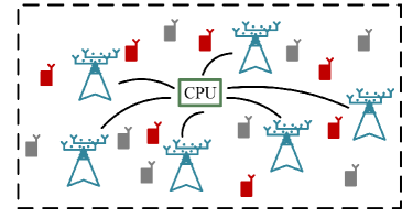
We consider an uplink cell-free massive MIMO-OFDM system where L APs serve a maximal number of K single-antenna UEs in the same time-frequency resource under the time-division duplex (TDD) mode. APs and UEs are randomly located over a large area. We assume each AP is equipped with two uniform linear arrays (ULAs). Each ULA comprises of N directional antennas and receives waves with the incidence angle in a range of 180180 degrees to avoid ambiguities in the array manifold. We denote M=NLM\!=\!NL. The sets of APs and UEs are denoted by ={0,1,,L1}\mathcal{L}\!=\!\{0,1,\cdots\!,L\!-\!1\} and 𝒦={0,1,,K1}\mathcal{K}\!=\!\{0,1,\cdots\!,K\!-\!1\}, respectively. The set of active UEs is denoted as 𝒦a\mathcal{K}_{a} with the size of KaKK_{a}\leq K. APs are connected to a CPU via an error-free fronthaul network, as shown in Fig. 1.

Refer to caption
Figure 1: Cell-free massive MIMO system. Active and inactive UEs are in red and gray, respectively.

We adopt OFDM with NcN_{c} subcarriers to combat time dispersive channels. The sampling duration is TsT_{s}. We employ Tsym=(Nc+Ncp)TsT_{\rm{sym}}=\left(N_{c}\!+\!N_{\rm{cp}}\right)T_{s} and Tc=NcTsT_{c}\!=\!N_{c}T_{s} to denote the OFDM symbol duration with and without cyclic prefix (CP), where NcpN_{\rm{cp}} denotes the number of symbols in CP. The CP duration Tcp=NcpTsT_{\rm{cp}}\!=\!N_{\rm{cp}}T_{s} is assumed to be longer than the maximum channel delay of UEs.

2.1 Channel Model in Space-Frequency Domain

In realistic outdoor wireless propagation environments, the channel angle spread is limited due to finite scattering clusters. Hence, we assume two ULAs in an AP separately receive waves from UEs with the mean angle of arrival (AoA) in a range of 180180 degrees, i.e., the waves from a UE are received by directional antennas of a ULA in each AP. Let 𝐠k,l,sβ\mathbf{g}_{k,l,s}^{\beta} denote the uplink channel response vector between the l-th AP and the k-th UE over the s-th subcarrier. We employ θ\theta to denote the incidence angle. 𝐠k,l,sβ\mathbf{g}_{k,l,s}^{\beta} can be modeled as [21, 23, 24]

𝐠k,l,sββk,l𝐠k,l,s=q=0Ncp1π2π2𝐯N(θ)exp{ȷ¯2πsTcτ}ak,lβ(θ,τ)δ(τqTs)dθN×1,\mathbf{g}_{k,l,s}^{\beta}\triangleq\sqrt{\beta_{k,l}}\;\mathbf{g}_{k,l,s}=\sum_{q=0}^{N_{\rm{cp}}-1}\int_{-\frac{\pi}{2}}^{\frac{\pi}{2}}\mathbf{v}_{N}(\theta)\exp\left\{-\overline{\jmath}2\pi\frac{s}{T_{c}}\tau\right\}a_{k,l}^{\beta}(\theta,\tau)\delta\left(\tau-qT_{s}\right)\mathrm{d}\theta\in\mathbb{C}^{N\times 1}, (1)

where βk,l\beta_{k,l} denotes the large-scale fading between the l-th AP and the k-th UE, 𝐠k,l,s\mathbf{g}_{k,l,s} denotes the small-scale fading, and ak,lβ(θ,τ)βk,lak,l(θ,τ)a_{k,l}^{\beta}(\theta,\tau)\triangleq\sqrt{\beta_{k,l}}a_{k,l}(\theta,\tau) represents the angle-delay domain channel gain function corresponding to the incidence angle θ\theta and delay τ\tau. If AP antennas are spaced with half of wavelength, the steering vector 𝐯N(θ)=[1,eȷ¯πsinθ,,eȷ¯π(N1)sinθ]T\mathbf{v}_{N}(\theta)=[1,e^{-\overline{\jmath}\pi\sin\theta},\cdots,e^{-\overline{\jmath}\pi(N-1)\sin\theta}]^{T}. The space-frequency domain channel response matrix between UE k and all APs over NcN_{c} subcarriers is denoted as

𝐆kβ[𝐆k,0β𝐆k,1β𝐆k,L1β]=[𝐠k,0,0β𝐠k,0,1β𝐠k,0,Nc1β𝐠k,1,0β𝐠k,1,1β𝐠k,1,Nc1β𝐠k,L1,0β𝐠k,L1,1β𝐠k,L1,Nc1β]=[𝐠k,0β𝐠k,1β𝐠k,Nc1β]M×Nc,\mathbf{G}_{k}^{\beta}\triangleq\begin{bmatrix}{\mathbf{G}_{k,0}^{\beta}}\\ {\mathbf{G}_{k,1}^{\beta}}\\ {\vdots}\\ {\mathbf{G}_{k,L-1}^{\beta}}\end{bmatrix}=\begin{bmatrix}{\mathbf{g}_{k,0,0}^{\beta}}&{\mathbf{g}_{k,0,1}^{\beta}}&\cdots&{\mathbf{g}_{k,0,N_{c}-1}^{\beta}}\\ {\mathbf{g}_{k,1,0}^{\beta}}&{\mathbf{g}_{k,1,1}^{\beta}}&\cdots&{\mathbf{g}_{k,1,N_{c}-1}^{\beta}}\\ {\vdots}&{\vdots}&{\ddots}&{\vdots}\\ {\mathbf{g}_{k,L-1,0}^{\beta}}&{\mathbf{g}_{k,L-1,1}^{\beta}}&\cdots&{\mathbf{g}_{k,L-1,N_{c}-1}^{\beta}}\end{bmatrix}=\begin{bmatrix}{\mathbf{g}_{k,0}^{\beta}}&{\mathbf{g}_{k,1}^{\beta}}&{\cdots}&{\mathbf{g}_{k,N_{c}-1}^{\beta}}\end{bmatrix}\in\mathbb{C}^{M\times N_{c}}, (2)

where 𝐆k,lβN×Nc{\mathbf{G}_{k,l}^{\beta}}\in\mathbb{C}^{N\times N_{c}} and 𝐠k,sβM×1{\mathbf{g}_{k,s}^{\beta}}\in\mathbb{C}^{M\times 1} are the space-frequency domain channel response matrix between the l-th AP and the k-th UE over NcN_{c} subcarriers, and the vector between all APs and the k-th UE over the s-th subcarrier, respectively. It is assumed that vec{𝐆kβ}𝒞𝒩(0,𝐑kβ)\operatorname{vec}\left\{\mathbf{G}_{k}^{\beta}\right\}\sim\mathcal{CN}\left(0,\mathbf{R}_{k}^{\beta}\right).

In this work, we consider the space-frequency domain correlation between the antennas of an AP and a UE over NcN_{c} subcarriers. We assume different UEs or APs are spatially separated by a few wavelengths, and the channel realizations between different UEs and an AP and the channel realizations between a UE and different APs are uncorrelated [22]. Besides, we assume the angle-delay domain channel gain function ak,l(θ,τ){a_{k,l}(\theta,\tau)} is uncorrelated [12, 23], i.e.,

𝔼{ak,l(θ,τ)ak,l(θ,τ)}=Pk,lA(θ)Pk,lD(τ)δ(kk)δ(ll)δ(θθ)δ(ττ),\mathbb{E}\left\{a_{k,l}(\theta,\tau)a^{\ast}_{k^{\prime},l^{\prime}}\left(\theta^{\prime},\tau^{\prime}\right)\right\}=P^{A}_{k,l}(\theta)P^{D}_{k,l}(\tau)\delta\left(k-k^{\prime}\right)\delta\left(l-l^{\prime}\right)\delta\left(\theta-\theta^{\prime}\right)\delta\left(\tau-\tau^{\prime}\right), (3)

where Pk,lA(θ)P^{A}_{k,l}(\theta) and Pk,lD(τ)P^{D}_{k,l}(\tau) represent the channel power azimuth spectrum (PAS) and power delay spectrum (PDS), respectively. Let ςk,l\varsigma_{k,l}, θk,l\theta_{k,l}, and ζk,l\zeta_{k,l} denote the angle spread, mean AoA, and delay spread between the k-th UE and the l-th AP, respectively. PAS and PDS are given by [25]

Pk,lA(θ)exp{2|θθk,l|/ςk,l}, for θ,θk,l[π/2,π/2],P^{A}_{k,l}(\theta)\propto\exp\left\{-{\sqrt{2}\left|\theta-\theta_{k,l}\right|}/{\varsigma_{k,l}}\right\},\text{ for }\theta,\theta_{k,l}\in[-\pi/2,\pi/2], (4)
Pk,lD(τ)exp{τ/ζk,l}, for τ[0,(Ncp1)Ts].P^{D}_{k,l}(\tau)\propto\exp\left\{-{\tau}/{\zeta_{k,l}}\right\},\text{ for }\tau\in\left[0,\left(N_{\mathrm{cp}}-1\right)T_{s}\right]. (5)

We assume the channel angle spreads between different UEs and APs are equal, i.e., ςk,l=ς\varsigma_{k,l}=\varsigma for k𝒦k\in\mathcal{K} and ll\in\mathcal{L}. Similarly, the delay spreads satisfy ζk,l=ζ\zeta_{k,l}=\zeta for k𝒦k\in\mathcal{K} and ll\in\mathcal{L}.

2.2 Channel Model in Angle-Delay Domain

Let 𝐇k,lββk,l𝐇k,lN×Ncp\mathbf{H}^{\beta}_{k,l}\triangleq\sqrt{\beta_{k,l}}\mathbf{H}_{k,l}\in\mathbb{C}^{N\times N_{\mathrm{cp}}} denote the angle-delay domain channel response matrix between the k-th UE and the l-th AP. Let 𝐇kβ[(𝐇k,0β)T(𝐇k,1β)T(𝐇k,L1β)T]T\mathbf{H}^{\beta}_{k}\triangleq\left[\left(\mathbf{H}^{\beta}_{k,0}\right)^{T}\left(\mathbf{H}^{\beta}_{k,1}\right)^{T}\cdots\left(\mathbf{H}^{\beta}_{k,L-1}\right)^{T}\right]^{T} and 𝐇k[𝐇k,0T𝐇k,1T𝐇k,L1T]T\mathbf{H}_{k}\triangleq\left[\mathbf{H}_{k,0}^{T}\;\mathbf{H}_{k,1}^{T}\cdots\mathbf{H}_{k,L-1}^{T}\right]^{T} denote the angle-delay domain channel response matrices between UE k and all APs with and without large-scale fading, respectively. Different elements in 𝐇kβ\mathbf{H}^{\beta}_{k} correspond to the channels for different incidence angles, delays or APs, which satisfy [12, 23]

𝔼{[𝐇kβ]m,q[𝐇kβ]m,q}=δ(mm)δ(qq)[𝚼kβ]m,q,\mathbb{E}\left\{\left[\mathbf{H}^{\beta}_{k}\right]_{m,q}\left[\mathbf{H}^{\beta}_{k}\right]_{m^{\prime},q^{\prime}}^{*}\right\}=\delta\left(m-m^{\prime}\right)\delta\left(q-q^{\prime}\right)\left[\bm{\Upsilon}^{\beta}_{k}\right]_{m,q}, (6)

where 𝚼kβ[(𝚼k,0β)T(𝚼k,1β)T(𝚼k,L1β)T]TM×Ncp\bm{\Upsilon}_{k}^{\beta}\!\triangleq\!\begin{bmatrix}\left(\bm{\Upsilon}^{\beta}_{k,0}\right)^{\!T}\!\!\!&\left(\bm{\Upsilon}^{\beta}_{k,1}\right)^{\!T}\!\!\!&\!\cdots\!\!\!&\left(\bm{\Upsilon}^{\beta}_{k,L-1}\right)^{\!T}\end{bmatrix}^{\!T}\!\in\!\mathbb{R}^{M\times N_{\mathrm{cp}}} is the angle-delay domain channel power spectrum between UE k and all APs. We define 𝚼k[𝚼k,0T𝚼k,1T𝚼k,L1T]TM×Ncp\bm{\Upsilon}_{k}\!\triangleq\!\begin{bmatrix}\bm{\Upsilon}^{T}_{k,0}\!&\bm{\Upsilon}^{T}_{k,1}\!\!&\!\cdots\!\!&\!\bm{\Upsilon}^{T}_{k,L-1}\end{bmatrix}^{\!T}\!\in\!\mathbb{R}^{M\times N_{\mathrm{cp}}}.

Wireless channels are sparse in many typical scenarios [26, 27]. In this work, we consider the angle-delay domain sparsity from a UE to all APs in a cell-free massive MIMO-OFDM system. Most elements in 𝚼kβ\bm{\Upsilon}_{k}^{\beta} are approximately 0 due to finite angle-delay spread.

2.3 Relationship between Space-Frequency Domain and Angle-Delay Domain Channels

Since the channel power lies in a finite number of delays due to limited scattering, channels are frequently correlated [23]. Considering most channel power is concentrated in a finite region of angles, channels between the antennas of an AP and a UE are spatially correlated [27]. Proposition 2.3 shows the relationship between the space-frequency domain channel covariance matrix and the angle-delay domain channel power spectrum in cell-free massive MIMO-OFDM systems. \proposition[] Define θn=arcsin(2nN1)\theta_{n}\!=\!\arcsin\left(\frac{2n}{N}-1\right) for n=0,1,,Nn=0,1,\cdots\!,N. Let [𝐕N×N]i,j1Nexp{ȷ¯πisinθn}\left[\mathbf{V}_{N\times N}\right]_{i,j}\triangleq\frac{1}{\sqrt{N}}\exp\left\{-\overline{\jmath}\pi i\sin\theta_{n}\right\}, 𝐕M×M𝐈L×L𝐕N×N\mathbf{V}_{M\times M}\triangleq\mathbf{I}_{L\times L}\otimes\mathbf{V}_{N\times N}, and [𝐅Nc×Ncp]s,q1Ncexp{ȷ¯2πsNcq}\left[\mathbf{F}_{N_{c}\times N_{\mathrm{cp}}}\right]_{s,q}\triangleq\frac{1}{\sqrt{N_{c}}}\exp\left\{-\overline{\jmath}2\pi\frac{s}{N_{c}}q\right\}. We have 𝐕N×NH𝐕N×N=N𝐈N×N\mathbf{V}_{N\times N}^{H}\mathbf{V}_{N\times N}\stackrel{{\scriptstyle N\rightarrow\infty}}{{=}}\mathbf{I}_{N\times N} and 𝐕M×MH𝐕M×M=N𝐈M×M\mathbf{V}_{M\times M}^{H}\mathbf{V}_{M\times M}\stackrel{{\scriptstyle N\rightarrow\infty}}{{=}}\mathbf{I}_{M\times M}. The channel power spectrum between the k-th UE and the l-th AP is denoted as 𝚼k,lβN×Ncp\bm{\Upsilon}_{k,l}^{\beta}\in\mathbb{R}^{N\times N_{\mathrm{cp}}} satisfying

[𝚼k,lβ]n,qβk,l[𝚼k,l]n,q=βk,lNNc(θn+1θn)Pk,lA(θn)Pk,lD(τq),\left[\bm{\Upsilon}_{k,l}^{\beta}\right]_{n,q}\triangleq\beta_{k,l}\left[\bm{\Upsilon}_{k,l}\right]_{n,q}=\beta_{k,l}NN_{c}\left(\theta_{n+1}-\theta_{n}\right)P^{A}_{k,l}(\theta_{n})P^{D}_{k,l}(\tau_{q}), (7)

where τq=qTs\tau_{q}=qT_{s} for q=0,1,,Ncp1q=0,1,\cdots,N_{\mathrm{cp}}-1. The relationship between the space-frequency domain channel covariance matrix and angle-delay domain channel power spectrum is given by

𝐑kβ=N(𝐅Nc×Ncp𝐕M×M)diag{vec{𝚼kβ}}(𝐅Nc×Ncp𝐕M×M)HMNc×MNc.\mathbf{R}^{\beta}_{k}\stackrel{{\scriptstyle N\rightarrow\infty}}{{=}}\left(\mathbf{F}_{N_{c}\times N_{\mathrm{cp}}}\otimes\mathbf{V}_{M\times M}\right)\operatorname{diag}\bigg{\{}\operatorname{vec}\left\{\bm{\Upsilon}_{k}^{\beta}\right\}\bigg{\}}\left(\mathbf{F}_{N_{c}\times N_{\mathrm{cp}}}\otimes\mathbf{V}_{M\times M}\right)^{H}\in\mathbb{C}^{MN_{c}\times MN_{c}}. (8)

The space-frequency domain channel response matrix 𝐆kβ\mathbf{G}_{k}^{\beta} can be decomposed as

𝐆kβ=N𝐕M×M𝐇kβ𝐅Nc×NcpT.\mathbf{G}_{k}^{\beta}\stackrel{{\scriptstyle N\rightarrow\infty}}{{=}}\mathbf{V}_{M\times M}\mathbf{H}_{k}^{\beta}\;\mathbf{F}^{T}_{N_{c}\times N_{\mathrm{cp}}}. (9)
Proof.

See A.

When NN is sufficiently large, the eigenvectors of space-frequency domain channel covariance matrices are independent of the locations of UEs and only depend on the AP antenna configurations. Eigenvalues can be approximated by the angle-delay domain channel power spectrum. Specifically, when ULAs are employed at each AP with antenna spacing of half-wavelength, 𝐕N×N\mathbf{V}_{N\times N} can be set to discrete Fourier transform (DFT) matrices with some matrix elementary operations. Since the dimension of 𝚼kβ\bm{\Upsilon}_{k}^{\beta} is much smaller than that of 𝐑kβ\mathbf{R}_{k}^{\beta} and most elements in 𝚼kβ\bm{\Upsilon}_{k}^{\beta} are approximately 0, we will estimate angle-delay domain channel parameters at first, and then obtain space-frequency domain channel parameters via (9). We assume angle-delay domain channel power spectrums are known by APs.

Proposition 2.3 is a generalization of existing results. It agrees with the results in [27] where channels are frequency-flat fading on a narrow-band subcarrier. It is consistent with the results in [24], where correlated channels in co-located systems are considered. The approximation is shown to be accurate enough when the number of antennas at the BS ranges from 64 to 512 in frequency-flat co-located massive MIMO channels [28].

3 Pilot Transmission Design with Pilot Assignment

UEs are sporadically active and far more than orthogonal pilots in crowded scenarios, which calls for proper design of uplink transmission scheme and pilot assignment scheme. We utilize APSP to increase the number of unique pilots as shown in Section 3.1. Besides, active UEs can be identified through pilot shift hopping patterns as introduced in Section 3.2. To better utilize channel characteristics and improve MSE-CE in correlated cell-free massive MIMO-OFDM systems, an APSP set allocation scheme is proposed in Section 3.3.

3.1 APSP and Channel Estimation

We assume channels are piece-wise constant over a coherence interval. The time coherence interval is assumed to be equal to the length of ZaZ_{a} OFDM symbols. The frequency coherence interval is assumed to be equal to 12ζ\frac{1}{2\zeta}. We assume ZZ OFDM symbols are used for pilot transmission and the remaining ZaZZ_{a}-Z OFDM symbols are for uplink data transmission.

During the training phase, all active UEs simultaneously transmit pilots to APs. The space-frequency domain signal received at the l-th AP is given by

𝐘l=ρpZk𝒦a𝐆k,lβ𝚽k+𝐖lN×NcZ,\mathbf{Y}_{l}=\sqrt{\rho_{p}Z}\sum_{k^{\prime}\in\mathcal{K}_{a}}\mathbf{G}_{k^{\prime},l}^{\beta}\mathbf{\Phi}_{k^{\prime}}+\mathbf{W}_{l}\in\mathbb{C}^{N\times N_{c}Z}, (10)

where ρp\rho_{p} is the normalized signal-to-noise ratio (SNR) in the training phase, 𝐖l\mathbf{W}_{l} is the additive white Gaussian noise (AWGN) matrix including i.i.d. 𝒞𝒩(0,1)\mathcal{CN}(0,1) elements, 𝐆k,lβ=𝐕N×N𝐇k,lβ𝐅Nc×NcpT\mathbf{G}_{k^{\prime},l}^{\beta}=\mathbf{V}_{N\times N}\mathbf{H}_{k^{\prime},l}^{\beta}\mathbf{F}^{T}_{N_{c}\times N_{\mathrm{cp}}}, and 𝚽k\mathbf{\Phi}_{k^{\prime}} is the pilot signal given in (11). We assume large-scale fading coefficients are known wherever required.

In cell-free massive MIMO-OFDM systems, the number of phase shift orthogonal pilots (PSOPs) is approximately ZNc/Ncp\lfloor ZN_{c}/N_{cp}\rfloor. Their phase shift differences are no less than the maximum channel delay of UEs to promise orthogonality of different pilots [29]. However, pilot contamination can be serious since UEs are far more than PSOPs. Hence, APSP is adopted in this work [24]. The pilot signal for the k-th UE over NcN_{c} subcarriers and ZZ OFDM symbols is

𝚽k[𝐔]ϕkZ,:(𝐃ϕk/Z𝚽b)Nc×NcZ,\mathbf{\Phi}_{k}\triangleq\left[\mathbf{U}\right]_{\left\langle\phi_{k}\right\rangle_{Z},:}\otimes\left(\mathbf{D}_{\left\lfloor\phi_{k}/Z\right\rfloor}\mathbf{\Phi}_{b}\right)\in\mathbb{C}^{N_{c}\times N_{c}Z}, (11)

where 𝐔\mathbf{U} is an arbitrary Z×ZZ\times Z dimensional unitary matrix, ϕk𝚿={0,1,,NcZ1}\phi_{k}\in\mathbf{\Psi}=\left\{0,1,\cdots,N_{c}Z-1\right\}, 𝐃i=diag{𝐟Nc,i}\mathbf{D}_{i}=\operatorname{diag}\left\{\mathbf{f}_{N_{c},i}\right\}, 𝐟Nc,i=[1exp{ȷ¯2πiNc}exp{ȷ¯2π(Nc1)iNc}]T\mathbf{f}_{N_{c},i}=\left[1\;\exp\left\{-\overline{\jmath}2\pi\frac{i}{N_{c}}\right\}\cdots\exp\left\{-\overline{\jmath}2\pi\frac{\left(N_{c}-1\right)i}{N_{c}}\right\}\right]^{T}, and 𝚽b\mathbf{\Phi}_{b} is a diagonal matrix satisfying 𝚽b𝚽bH=𝐈Nc×Nc\mathbf{\Phi}_{b}\mathbf{\Phi}_{b}^{H}=\mathbf{I}_{N_{c}\times N_{c}}, which is the basic pilot matrix shared by all UEs. Then we have, for k,k𝒦\forall k,k^{\prime}\in\mathcal{K},

𝚽k𝚽kH=(a)([𝐔]ϕkZ,:[𝐔]ϕkZ,:H)(𝐃ϕk/Z𝐃ϕk/ZH)=δ(ϕkZϕkZ)𝐃ϕk/Zϕk/Z,\mathbf{\Phi}_{k^{\prime}}\mathbf{\Phi}_{k}^{H}\stackrel{{\scriptstyle(\mathrm{a})}}{{=}}\left([\mathbf{U}]_{\left\langle\phi_{k^{\prime}}\right\rangle_{Z},:}[\mathbf{U}]_{\left\langle\phi_{k}\right\rangle_{Z},:}^{H}\right)\otimes\left(\mathbf{D}_{\left\lfloor\phi_{k^{\prime}}/Z\right\rfloor}\mathbf{D}_{\left\lfloor\phi_{k}/Z\right\rfloor}^{H}\right)=\delta\left(\left\langle\phi_{k^{\prime}}\right\rangle_{Z}-\left\langle\phi_{k}\right\rangle_{Z}\right)\mathbf{D}_{\left\lfloor{\phi_{k^{\prime}}}/{Z}\right\rfloor-\left\lfloor{\phi_{k}}/{Z}\right\rfloor}, (12)

where (a) follows from the properties of Kronecker product, i.e., (𝐀𝐁)(𝐂𝐃)=(𝐀𝐂)(𝐁𝐃)(\mathbf{A}\otimes\mathbf{B})(\mathbf{C}\otimes\mathbf{D})=(\mathbf{A}\mathbf{C})\otimes(\mathbf{BD}) and (𝐀𝐁)H=𝐀H𝐁H(\mathbf{A}\otimes\mathbf{B})^{H}=\mathbf{A}^{H}\otimes\mathbf{B}^{H}. For the APSP, phase shifts are divided into ZZ groups. The group index is ϕkZ\left\langle\phi_{k}\right\rangle_{Z}. There is no pilot interference if UEs use phase shifts in different groups.

Based on (10), (11), and (12), after decorrelation, we have

𝐘ˇk,l\displaystyle\check{\mathbf{Y}}_{k,l} =1ρpZβk,l𝐕N×NH𝐘l𝚽kH𝐅Nc×Ncp\displaystyle=\frac{1}{\sqrt{\rho_{p}Z\beta_{k,l}}}\mathbf{V}_{N\times N}^{H}\mathbf{Y}_{l}\mathbf{\Phi}_{k}^{H}\mathbf{F}_{N_{c}\times N_{\mathrm{cp}}}^{\ast}
=𝐇k,l+1βk,lk𝒦a\{k}δ(ϕkZϕkZ)𝐇k,lβ𝐅Nc×NcpT𝐃ϕk/Zϕk/Z𝐅Nc×Ncp+1ρpZβk,l𝐖ˇk,l\displaystyle={{\mathbf{H}}_{k,l}}+\frac{1}{\sqrt{{{\beta}_{k,l}}}}\sum\limits_{{k}^{\prime}\in{{\mathcal{K}}_{a}}\backslash\left\{k\right\}}\!\!\!\!\delta\left(\left\langle\phi_{k^{\prime}}\right\rangle_{Z}-\left\langle\phi_{k}\right\rangle_{Z}\right)\mathbf{H}_{{k}^{\prime},l}^{\beta}\mathbf{F}_{{{N}_{c}}\times{{N}_{\mathrm{cp}}}}^{T}\mathbf{D}_{\left\lfloor{\phi_{k^{\prime}}}\!/{Z}\right\rfloor-\left\lfloor{\phi_{k}}/{Z}\right\rfloor}\mathbf{F}_{\!{{N}_{c}}\times{{N}_{\mathrm{cp}}}}^{\ast}+\frac{1}{\sqrt{{{\rho}_{p}}Z{{\beta}_{k,l}}}}{\check{\mathbf{W}}_{k,l}}
=𝐇k,l+1βk,lk𝒦a\{k}δ(ϕkZϕkZ)𝐇k,lβ,ϕk/Zϕk/Z+1ρpZβk,l𝐖ˇk,l,\displaystyle={{\mathbf{H}}_{k,l}}+\frac{1}{\sqrt{{{\beta}_{k,l}}}}\sum\limits_{{k}^{\prime}\in{{\mathcal{K}}_{a}}\backslash\left\{k\right\}}\!\!\!\!\delta\left(\left\langle\phi_{k^{\prime}}\right\rangle_{Z}-\left\langle\phi_{k}\right\rangle_{Z}\right)\mathbf{H}_{{k}^{\prime},l}^{\beta,\left\lfloor{\phi_{k^{\prime}}}/{Z}\right\rfloor-\left\lfloor{\phi_{k}}/{Z}\right\rfloor}+\frac{1}{\sqrt{{{\rho}_{p}}Z{{\beta}_{k,l}}}}{\check{\mathbf{W}}_{k,l}}, (13)

where 𝐖ˇk,l{\check{\mathbf{W}}_{k,l}} includes i.i.d. 𝒞𝒩(0,1)\mathcal{CN}(0,1) entrys due to unitary transformation. Define the permutation matrix 𝚪Nci=[𝟎𝐈(NciNc)×(NciNc)𝐈iNc×iNc𝟎]\mathbf{\Gamma}^{i}_{N_{c}}=\left[\begin{array}[]{cc}{\mathbf{0}}&{\mathbf{I}_{\left(N_{c}-\left\langle i\right\rangle_{N_{c}}\right)\times\left(N_{c}-\left\langle i\right\rangle_{N_{c}}\right)}}\\ {\mathbf{I}_{\left\langle i\right\rangle_{N_{c}}\times\left\langle i\right\rangle_{N_{c}}}}&{\mathbf{0}}\end{array}\right]. Then, 𝐇k,lβ,ϕk/Zϕk/Z\mathbf{H}_{{k}^{\prime},l}^{\beta,\left\lfloor{\phi_{k^{\prime}}}/{Z}\right\rfloor-\left\lfloor{\phi_{k}}/{Z}\right\rfloor} can be expressed as

𝐇k,lβ,ϕk/Zϕk/Z=𝐇k,lβ𝐈Nc×NcpT𝚪Ncϕk/Zϕk/Z𝐈Nc×Ncp.\mathbf{H}_{{k}^{\prime},l}^{\beta,\left\lfloor{\phi_{k^{\prime}}}/{Z}\right\rfloor-\left\lfloor{\phi_{k}}/{Z}\right\rfloor}=\mathbf{H}_{k^{\prime},l}^{\beta}\mathbf{I}_{N_{c}\times N_{\mathrm{cp}}}^{T}\mathbf{\Gamma}^{{\left\lfloor{\phi_{k^{\prime}}}/{Z}\right\rfloor-\left\lfloor{\phi_{k}}/{Z}\right\rfloor}}_{N_{c}}\mathbf{I}_{N_{c}\times N_{\mathrm{cp}}}. (14)

The power spectrum of (14) is given by

𝚼k,lβ,ϕk/Zϕk/Z\displaystyle\mathbf{\Upsilon}_{{{k}^{\prime},l}}^{\beta,{\left\lfloor{\phi_{k^{\prime}}}/{Z}\right\rfloor-\left\lfloor{\phi_{k}}/{Z}\right\rfloor}} =𝔼{𝐇k,lβ,ϕk/Zϕk/Z(𝐇k,lβ,ϕk/Zϕk/Z)}\displaystyle=\mathbb{E}\left\{\mathbf{H}_{{k}^{\prime},l}^{\beta,{\left\lfloor{\phi_{k^{\prime}}}/{Z}\right\rfloor-\left\lfloor{\phi_{k}}/{Z}\right\rfloor}}\odot{{\left(\mathbf{H}_{{k}^{\prime},l}^{\beta,{\left\lfloor{\phi_{k^{\prime}}}/{Z}\right\rfloor-\left\lfloor{\phi_{k}}/{Z}\right\rfloor}}\right)}^{\ast}}\right\}
=𝚼k,lβ𝐈Nc×NcpT𝚪Ncϕk/Zϕk/Z𝐈Nc×Ncp.\displaystyle=\mathbf{\Upsilon}_{k^{\prime},l}^{\beta}\mathbf{I}_{N_{c}\times N_{\mathrm{cp}}}^{T}\mathbf{\Gamma}_{{{N}_{c}}}^{{\left\lfloor{\phi_{k^{\prime}}}/{Z}\right\rfloor-\left\lfloor{\phi_{k}}/{Z}\right\rfloor}}{{\mathbf{I}}_{{{N}_{c}}\times{{N}_{\mathrm{cp}}}}}. (15)

Define 𝚼kβ,ϕk/Zϕk/Z[(𝚼k,0β,ϕk/Zϕk/Z)T(𝚼k,1β,ϕk/Zϕk/Z)T(𝚼k,L1β,ϕk/Zϕk/Z)T]T{\mathbf{\Upsilon}}_{k^{\prime}}^{\beta,{\left\lfloor{\phi_{k^{\prime}}}/{Z}\right\rfloor-\left\lfloor{\phi_{k}}/{Z}\right\rfloor}}\triangleq\begin{bmatrix}\left({\mathbf{\Upsilon}}_{k^{\prime},0}^{\beta,{\left\lfloor{\phi_{k^{\prime}}}/{Z}\right\rfloor-\left\lfloor{\phi_{k}}/{Z}\right\rfloor}}\right)^{T}&\left({\mathbf{\Upsilon}}_{k^{\prime},1}^{\beta,{\left\lfloor{\phi_{k^{\prime}}}/{Z}\right\rfloor-\left\lfloor{\phi_{k}}/{Z}\right\rfloor}}\right)^{T}&\cdots&\left({\mathbf{\Upsilon}}_{k^{\prime},L-1}^{\beta,{\left\lfloor{\phi_{k^{\prime}}}/{Z}\right\rfloor-\left\lfloor{\phi_{k}}/{Z}\right\rfloor}}\right)^{T}\end{bmatrix}^{T}.

Channels are estimated in a decentralized fashion in cell-free massive MIMO-OFDM systems, i.e., each AP autonomously estimates channels without interchanging information [5]. For an AP, the channel estimation is performed in an element-wise manner in the angle-delay domain. The minimum mean-square error (MMSE) estimate of [𝐇k,l]i,j\left[{{\mathbf{H}}_{k,l}}\right]_{i,j} is

[𝐇^k,l]i,j=[𝚼k,lβ]i,jk𝒦aδ(ϕkZϕkZ)[𝚼k,lβ,ϕk/Zϕk/Z]i,j+1ρpZ[𝐘ˇk,l]i,j.{{\left[{{\widehat{\mathbf{H}}}_{k,l}}\right]}_{i,j}}=\frac{{{\left[\mathbf{\Upsilon}_{k,l}^{\beta}\right]}_{i,j}}}{\sum\limits_{{k}^{\prime}\in{{\mathcal{K}}_{a}}}\delta\left(\left\langle\phi_{k^{\prime}}\right\rangle_{Z}-\left\langle\phi_{k}\right\rangle_{Z}\right){{{\left[\mathbf{\Upsilon}_{{k}^{\prime},l}^{\beta,{\left\lfloor\!{\phi_{k^{\prime}}}/{Z}\right\rfloor-\left\lfloor\!{\phi_{k}}/{Z}\right\rfloor}}\right]}_{i,j}}+\frac{1}{{{\rho}_{p}Z}}}}{{\left[{\check{\mathbf{Y}}_{k,l}}\right]}_{i,j}}. (16)

Denote by 𝐇~k,l=𝐇k,l𝐇^k,l{{\widetilde{\mathbf{H}}}_{k,l}}={{{\mathbf{H}}}_{k,l}}-{{\widehat{\mathbf{H}}}_{k,l}} the channel estimation error. Based on the property of MMSE estimation, 𝐇~k,l{{\widetilde{\mathbf{H}}}_{k,l}} is independent of 𝐇^k,l{{\widehat{\mathbf{H}}}_{k,l}}, and the MSE-CE is shown as

[𝚵k,l]i,j𝔼{[𝐇~k,l]i,j[𝐇~k,l]i,j}=[𝚼k,l]i,j[𝚼k,l]i,j[𝚼k,lβ]i,jk𝒦aδ(ϕkZϕkZ)[𝚼k,lβ,ϕk/Zϕk/Z]i,j+1ρpZ.{{\left[{\mathbf{\Xi}}_{k,l}\right]}_{i,j}}\!\triangleq\mathbb{E}\left\{{{\left[{{\widetilde{\mathbf{H}}}_{k,l}}\right]}_{i,j}}{{\left[{{\widetilde{\mathbf{H}}}_{k,l}}\right]}^{\ast}_{i,j}}\right\}=\left[{{{\mathbf{\Upsilon}}}_{k,l}}\right]_{i,j}-\frac{{{\left[{{\mathbf{\Upsilon}}_{k,l}}\right]}_{i,j}}{{\left[\mathbf{\Upsilon}_{k,l}^{\beta}\right]}_{i,j}}}{\sum\limits_{{k}^{\prime}\in{{\mathcal{K}}_{a}}}{\!\delta\left(\left\langle\phi_{k^{\prime}}\right\rangle_{\!Z}\!-\left\langle\phi_{k}\right\rangle_{Z}\right){{\left[\mathbf{\Upsilon}_{{k}^{\prime},l}^{\beta,{\left\lfloor{\phi_{k^{\prime}}}/{Z}\right\rfloor-\left\lfloor{\phi_{k}}/{Z}\right\rfloor}}\right]}_{\!i,j}}}\!+\!\frac{1}{{{\rho}_{p}}Z}}. (17)

Define 𝚵kβ[βk,0𝚵k,0Tβk,1𝚵k,1Tβk,L1𝚵k,L1T]T\bm{\Xi}_{k}^{\beta}\triangleq\begin{bmatrix}\beta_{k,0}\bm{\Xi}_{k,0}^{T}&\beta_{k,1}\bm{\Xi}_{k,1}^{T}&\cdots&\beta_{k,L-1}\bm{\Xi}_{k,L-1}^{T}\end{bmatrix}^{T}.

Refer to caption
Figure 2: Illustration of the transmission frame. In this example, the hopping pattern for a given UE is {a,a,b,,c}\left\{a,a,b,\cdots,c\right\}. Pilot signals among NcN_{c} subcarriers are formulated based on this pattern, and transmitted during the pilot transmission phase. Data codewords are transmitted afterwards.

3.2 UE Identification

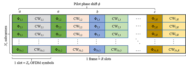
Pilot contamination is unavoidable in crowded scenarios. In this case, transmitting UEs cannot be identified in a slot, and we have to resort to the information among some slots. In this work, the uplink transmission phase is divided into frames consisting of RR slots, as shown in Fig. 2. Each slot comprises ZaZ_{a} OFDM symbols. The phase shifts of pilot signals among RR slots, i.e., the hopping patterns, form the identification basis of active UEs. When PSOPs are utilized, the number of UEs that can be identified is ZNc/NcpR\lfloor ZN_{c}/N_{cp}\rfloor^{R}. It can be further increased if APSPs are adopted due to channel sparsity. Hence, we assume each UE has a unique and non-orthogonal pseudo-random hopping pattern, which are known by APs and CPU in advance.

Assuming the activation probability of UEs is pap_{a}, the probability of having KaK_{a} active UEs among K UEs is given by

p(Ka|K)=(KKa)paKa(1pa)KKa.p(K_{a}|K)={K\choose{K_{a}}}p_{a}^{K_{a}}(1-p_{a})^{K-K_{a}}. (18)

When a UE is active, it selects the pilot phase shift based on its hopping pattern. Next, it formulates corresponding pilot over NcN_{c} subcarriers based on (11) and transmits this pilot during the pilot transmission phase. Data codewords are transmitted afterwards. At the receiver, APs identify hopping patterns by running a correlation decoder across RR slots to detect transmitting UEs. Normalized Maximum Ratio Combining (MRC) is applied to the data at APs and the outputs are merged based on the identified hopping patterns. Since APs can know which UEs are active and what they transmit after RR slots, this scheme is suitable for delay-tolerant mMTC.

3.3 APSP Set Allocation

In cell-free massive MIMO-OFDM systems, for a UE, the APs far from it cannot contribute significantly to the channel estimation performance and spatial diversity gains due to heavy path loss. Besides, the transfer of data between APs and CPU causes much fronthaul energy consumption. Hence, in order to improve channel estimation performance and save fronthaul energy consumption, each UE should be served by a group of APs but not all APs within the network [30]. Hence, before allocating APSP set for each UE, AP selection is performed at CPU [16]. The set of APs selected to serve the k-th UE is denoted as k\mathcal{B}_{k}\subseteq\mathcal{L} satisfying b=0|k|1β¯k,bl=0L1βk,lλ\sum_{b=0}^{\left|\mathcal{B}_{k}\right|-1}\overline{\beta}_{k,b}\geq\sum_{l=0}^{L-1}\beta_{k,l}\lambda, where {β¯k,0,β¯k,1,,β¯k,L1}\left\{\overline{\beta}_{k,0},\overline{\beta}_{k,1},\cdots,\overline{\beta}_{k,L-1}\right\} includes large-scale fading coefficients between UE k and APs in descending order, and λ\lambda is assumed to be equal for all UEs. The APs belonging to k\mathcal{B}_{k} need to estimate channels and decode signals of UE kk. The set of UEs served by AP l is denoted as 𝒟l\mathcal{D}_{l}.

The sporadic and independent activation of UEs and the construction of pseudo-random hopping patterns can be modeled as the process that each active UE randomly selects a pilot phase shift from its allocated set in each slot [11]. We obtain the probability of having KaK_{a} active UEs in (18), but it is still uncertain which KaK_{a} UEs are active and which phase shifts they select. To quantify these uncertainties, we employ 𝒰𝒦a={𝒰𝒦a0,𝒰𝒦a1,,𝒰𝒦aN𝒦a1}{{\mathcal{U}}_{{{\mathcal{K}}_{a}}}}=\left\{\mathcal{U}_{{{\mathcal{K}}_{a}}}^{0},\mathcal{U}_{{{\mathcal{K}}_{a}}}^{1},\cdots\!,\mathcal{U}_{{{\mathcal{K}}_{a}}}^{{{N}_{{{\mathcal{K}}_{a}}}}-1}\right\} to denote all possible sets of KaK_{a} active UEs. The j-th element in 𝒰𝒦ai{{\mathcal{U}}^{i}_{{{\mathcal{K}}_{a}}}} is denoted as 𝒦ai,j{{\mathcal{K}}^{i,j}_{a}}. In a slot, all possible choices of phase shifts for UEs in 𝒰𝒦ai{{\mathcal{U}}^{i}_{{{\mathcal{K}}_{a}}}} are denoted as 𝒫i={𝒫i0,𝒫i1,,𝒫iNϕ1}{{\mathcal{P}}_{i}}=\left\{\mathcal{P}_{i}^{0},\mathcal{P}_{i}^{1},\cdots,\mathcal{P}_{i}^{{{N}_{\phi}-1}}\right\}. Assuming the pp-th choice of shifts is considered, the phase shift of UE 𝒦ai,j{{\mathcal{K}}^{i,j}_{a}} is denoted as 𝒫i,jp\mathcal{P}_{i,j}^{p}. We assume νk,l\nu_{k,l} is equal to 11 when the l-th AP is selected to serve the kk-th UE and is equal to 0 otherwise. Let 𝚼kβ,0[νk,0βk,0𝚼k,0Tνk,1βk,1𝚼k,1Tνk,L1βk,L1𝚼k,L1T]T\bm{\Upsilon}_{k}^{\beta,0}\triangleq\begin{bmatrix}\nu_{k,0}\beta_{k,0}\bm{\Upsilon}^{T}_{k,0}&\nu_{k,1}\beta_{k,1}\bm{\Upsilon}^{T}_{k,1}&\cdots&\nu_{k,L-1}\beta_{k,L-1}\bm{\Upsilon}^{T}_{k,L-1}\end{bmatrix}^{T} and 𝚼k0[νk,0𝚼k,0Tνk,1𝚼k,1Tνk,L1𝚼k,L1T]T\bm{\Upsilon}_{k}^{0}\triangleq\begin{bmatrix}\nu_{k,0}\bm{\Upsilon}^{T}_{k,0}&\nu_{k,1}\bm{\Upsilon}^{T}_{k,1}&\cdots&\nu_{k,L-1}\bm{\Upsilon}^{T}_{k,L-1}\end{bmatrix}^{T}. Based on the channel estimation analysis in Section 3.1, we obtain the MSE-CE of UE 𝒦ai,j{{\mathcal{K}}^{i,j}_{a}} averaged over its serving APs and NcN_{c} subcarriers

ε𝒦ai,j,p0=1Nc|𝒦ai,j|m=0M1q=0Ncp1{[𝚼𝒦ai,j0]m,q[𝚼𝒦ai,j0]m,q[𝚼𝒦ai,jβ,0]m,qj=0Ka1δ(𝒫i,jpZ𝒫i,jpZ)[𝚼𝒦ai,jβ,𝒫i,jp/Z𝒫i,jp/Z]m,q+1ρpZ}.\varepsilon^{0}_{{{\mathcal{K}}^{i,j}_{a}},p}\!=\!{\frac{1}{{{N}_{c}}{\left|\mathcal{B}_{{\mathcal{K}}^{i,j}_{a}}\right|}}}{\sum\limits_{m=0}^{M-1}{\sum\limits_{q=0}^{{{N}_{\mathrm{cp}}}-1}{\!\left\{\!{{\left[\mathbf{\Upsilon}^{0}_{\mathcal{K}_{a}^{i,j}}\right]}_{m,q}}\!-\!\frac{{{\left[\mathbf{\Upsilon}^{0}_{\mathcal{K}_{a}^{i,j}}\right]}_{m,q}}{{\left[\mathbf{\Upsilon}_{\mathcal{K}_{a}^{i,j}}^{\beta,0}\right]}_{m,q}}}{\sum\limits_{j^{\prime}=0}^{K_{a}-1}\!\delta\!\left(\left\langle\mathcal{P}_{i,j^{\prime}}^{p}\right\rangle_{\!Z}\!-\!\left\langle\mathcal{P}_{i,j}^{p}\right\rangle_{\!Z}\right)\!{{{\left[\mathbf{\Upsilon}_{\mathcal{K}_{a}^{i,{j}^{\prime}}}^{\beta,\left\lfloor{\mathcal{P}_{i,j^{\prime}}^{p}}\!/{Z}\right\rfloor-\left\lfloor{\mathcal{P}_{i,j}^{p}}/{Z}\right\rfloor}\right]}_{m,q}}\!\!+\!\frac{1}{{{\rho}_{p}}Z}}}\right\}}}}. (19)

We average (19) over all possible sets of active UEs, all UEs in the set, and all types of phase shift selection. We obtain

𝔼𝒰,𝒦a,𝒫(ε0)=i=0N𝒦a1j=0Ka1p=0Nϕ1ε𝒦ai,j,p0N𝒦aKaNϕ.{{\mathbb{E}}_{\mathcal{U},{{\mathcal{K}}_{{a}}},\mathcal{P}}}(\varepsilon^{0})=\sum\limits_{i=0}^{{{N}_{{{\mathcal{K}}_{a}}}-1}}{\sum\limits_{j=0}^{{{K}_{a}-1}}{\sum\limits_{p=0}^{{{N}_{\phi}-1}}{\frac{\varepsilon^{0}_{{{\mathcal{K}}^{i,j}_{a}},p}}{{{N}_{{{\mathcal{K}}_{a}}}}{{K}_{a}}{{N}_{\phi}}}}}}. (20)

Then we calculate the expected value of (20) accounting for the number of active UEs and obtain

ε¯0=Ka=1Kp(Ka|K)𝔼𝒰,𝒦a,𝒫(ε0).\overline{\varepsilon}^{0}=\sum\limits_{K_{a}=1}^{K}{p(K_{a}|K){{\mathbb{E}}_{\mathcal{U},{{\mathcal{K}}_{{a}}},\mathcal{P}}}(\varepsilon^{0})}. (21)

The channel estimation performance suffers from pilot interference. In Proposition 3.3, we show that the effect of pilot interference can be eliminated by proper APSP set allocation for UEs. Phase shifts in the APSP set of each UE are used to form the unique pilot phase shift hopping pattern for it. In correlated channels, many elements in 𝚼kβ\mathbf{\Upsilon}_{k}^{\beta} are approximately 0, which is the physical basis of the APSP set allocation scheme. \proposition[] The minimum value of 𝔼𝒰,𝒦a,𝒫(ε0){{\mathbb{E}}_{\mathcal{U},{{\mathcal{K}}_{{a}}},\mathcal{P}}}(\varepsilon^{0}) and ε¯0\overline{\varepsilon}^{0} are given by

[𝔼𝒰,𝒦a,𝒫(ε0)]min=1KNck=0K1m=0M1q=0Ncp11|k|([𝚼k0]m,q[𝚼k0]m,q[𝚼kβ,0]m,q[𝚼kβ]m,q+1ρpZ),\left[{{\mathbb{E}}_{\mathcal{U},{{\mathcal{K}}_{{\!a}}},\mathcal{P}}}(\varepsilon^{0})\right]_{\min}={\frac{1}{K{{N}_{c}}}}\sum\limits_{k=0}^{{K-1}}{\sum\limits_{m=0}^{M-1}{\sum\limits_{q=0}^{{{N}_{\mathrm{cp}}}-1}{\frac{1}{\left|\mathcal{B}_{k}\right|}}{\left({{\left[\mathbf{\Upsilon}_{k}^{0}\right]}_{m,q}}-\frac{{{\left[\mathbf{\Upsilon}_{k}^{0}\right]}_{m,q}}{{\left[\mathbf{\Upsilon}_{k}^{\beta,0}\right]}_{m,q}}}{{{\left[\mathbf{\Upsilon}_{k}^{\beta}\right]}_{m,q}}+\frac{1}{{{\rho}_{p}Z}}}\right)}}}, (22)
ε¯min0=Ka=1Kp(Ka|K)[𝔼𝒰,𝒦a,𝒫(ε0)]min,{{{\overline{\varepsilon}}}_{\min}^{0}}=\sum\limits_{K_{a}=1}^{K}{p(K_{a}|K)\left[{{\mathbb{E}}_{\mathcal{U},{{\mathcal{K}}_{{\!a}}},\mathcal{P}}}(\varepsilon^{0})\right]_{\min}}, (23)

and the minimum is achieved under the condition that for k,k𝒦\forall k,k^{\prime}\in\mathcal{K} and kkk\neq k^{\prime},

δ(ϕkZϕkZ)𝚼k0𝚼k0𝚼kβ,ϕk/Zϕk/Z=𝟎M×Ncp.\delta\left(\left\langle{{\phi}_{{{k}^{\prime}}}}\right\rangle_{Z}-\left\langle{{\phi}_{{{k}}}}\right\rangle_{Z}\right)\mathbf{\Upsilon}^{0}_{k}\odot\mathbf{\Upsilon}^{0}_{k}\odot\mathbf{\Upsilon}_{{{k}^{\prime}}}^{\beta,\left\lfloor{{\phi}_{{{k}^{\prime}}}}/Z\right\rfloor-\left\lfloor{{\phi}_{{{k}}}}/Z\right\rfloor}=\mathbf{0}_{M\times N_{\mathrm{cp}}}. (24)
Proof.

See B.

When APSPs are used, phase shifts are divided into ZZ groups. There is no pilot interference for UEs using shifts in different groups. Channel estimation of a UE is affected by interference from other UEs in the same group exhibiting corresponding cyclic shifts in the delay domain as shown in (3.1). δ(ϕkZϕkZ)𝚼kβ,ϕk/Zϕk/Z\delta\left(\left\langle{{\phi}_{{{k}^{\prime}}}}\right\rangle_{Z}\!-\!\left\langle{{\phi}_{{{k}}}}\right\rangle_{Z}\right)\mathbf{\Upsilon}_{{{k}^{\prime}}}^{\beta,\left\lfloor{{\phi}_{{{k}^{\prime}}}}/Z\right\rfloor-\left\lfloor{{\phi}_{k}}/Z\right\rfloor} is the angle-delay domain channel power spectrum interference from UE kk^{\prime} to UE kk exhibiting cyclic shifts. By proper pilot allocation based on (24), there can be no overlapping between δ(ϕkZϕkZ)𝚼kβ,ϕk/Zϕk/Z\delta\left(\left\langle{{\phi}_{{{k}^{\prime}}}}\right\rangle_{Z}\!-\!\left\langle{{\phi}_{{{k}}}}\right\rangle_{Z}\right)\mathbf{\Upsilon}_{{{k}^{\prime}}}^{\beta,\left\lfloor{{\phi}_{{{k}^{\prime}}}}/Z\right\rfloor-\left\lfloor{{\phi}_{k}}/Z\right\rfloor} and 𝚼k0\mathbf{\Upsilon}_{k}^{0}, i.e., the effect of pilot interference can be mitigated and ε¯0\overline{\varepsilon}^{0} can be minimized. In crowded correlated cell-free massive MIMO-OFDM systems, we can allocate an APSP set for each UE to reduce ε¯0{{{\overline{\varepsilon}}}^{0}}. This problem can be formulated as

min𝒴k,k𝒦ε¯0s.t.     0ϕk,cNcZ1fork𝒦,0c|𝒴|1ϕk,cfork𝒦,0c|𝒴|1,\begin{split}&\min_{\mathcal{Y}_{k},k\in\mathcal{K}}\;\;\;\overline{\varepsilon}^{0}\\ &\;\;\>{\rm{s.t.}}\;\;\;\;\;0\leq\phi_{k,c}\leq N_{c}Z-1~{}~{}\text{for}~{}k\in\mathcal{K},~{}0\leq c\leq\left|\mathcal{Y}\right|-1\\ &\>\;\;\;\;\;\;\;\;\;\;\;\phi_{k,c}\in\mathbb{Z}~{}~{}\text{for}~{}k\in\mathcal{K},~{}0\leq c\leq\left|\mathcal{Y}\right|-1,\end{split} (25)

where 𝒴k={ϕk,0,ϕk,1,,ϕk,|𝒴|1}\mathcal{Y}_{k}=\left\{\phi_{k,0},\phi_{k,1},\cdots\!,\phi_{k,\left|\mathcal{Y}\right|-1}\right\} is the APSP set allocated for the kk-th UE.

This problem is combinatorial and can be solved through an exhaustive search with large complexity. Importantly, the problem can be simplified if we aim at satisfying the condition in (24) as much as possible. First, we define ξ(𝐀,𝐁)\xi\left(\mathbf{A},\mathbf{B}\right) to measure the overlap degree between two non-negative matrices 𝐀,𝐁\mathbf{A},\mathbf{B}. When 𝐀=𝟎\mathbf{A}=\mathbf{0} or 𝐁=𝟎\mathbf{B}=\mathbf{0}, ξ(𝐀,𝐁)0\xi\left(\mathbf{A},\mathbf{B}\right)\triangleq 0. When 𝐀,𝐁𝟎\mathbf{A},\mathbf{B}\neq\mathbf{0}, we have

ξ(𝐀,𝐁)|i,j[𝐀𝐁]i,j|i,j[𝐀]i,j2i,j[𝐁]i,j2[0,1].\xi\left(\mathbf{A},\mathbf{B}\right)\triangleq\frac{\left|\sum\nolimits_{i,j}{{{\left[\mathbf{A}\odot\mathbf{B}\right]}_{i,j}}}\right|}{\sqrt{\sum\nolimits_{i,j}{\left[\mathbf{A}\right]_{i,j}^{2}}}\cdot\sqrt{\sum\nolimits_{i,j}{\left[\mathbf{B}\right]_{i,j}^{2}}}}\in\left[0,1\right]. (26)

In Algorithm 1, k-means clustering method is utilized to partition KK UEs into JJ clusters. Next, APSP set is allocated for each UE to make the effect of pilot interference from other UEs in the same cluster as small as possible. Algorithm 1 should be performed before pilot transmission, i.e., without the knowledge of UEs’ activity. Hence, it is computed at CPU assuming all UEs are active and their statistical CSI is known. Hence, this scheme is insensitive to the active pattern of UEs and does not need to be recomputed frequently.

Algorithm 1 APSP Set Allocation Algorithm
0:  The angle-delay domain channel power spectrum {𝚼k:k𝒦}\{\mathbf{\Upsilon}_{k}:k\in\mathcal{K}\}; the threshold λ\lambda and γ\gamma; the phase shift set 𝚿\mathbf{\Psi}; the large-scale fading 𝜷k[βk,0βk,1βk,L1]\bm{\beta}_{k}\triangleq\left[\beta_{k,0}\!\;\;\beta_{k,1}\cdots\beta_{k,L-1}\right] for k𝒦\forall k\in\mathcal{K}.
0:  The APSP set allocated to each UE {𝒴k,k𝒦}\left\{\mathcal{Y}_{k},k\in\mathcal{K}\right\}.
1:  Centroids are randomly chosen as 𝜷~jL×1\tilde{\bm{\beta}}_{j}\in\mathbb{C}^{L\times 1} for j=0,1,,J1j=0,1,\cdots,J-1
2:  For k𝒦\forall k\in\mathcal{K}, UE kk is assigned to the cluster with maxj=0,1,,J1ξ(𝜷k,𝜷~j)\max\limits_{j=0,1,\cdots,J-1}\xi\left(\bm{\beta}_{k},\tilde{\bm{\beta}}_{j}\right)
3:  Centroids are updated by averaging over UEs belonging to respective clusters and UEs are reassigned until the assignments no longer change. Denote 𝒞j\mathcal{C}_{j} as the set of UEs belonging to the jj-th cluster
4:  for j=0,1,,J1j=0,1,\cdots,J-1 do
5:     |𝒴|\left|\mathcal{Y}\right| shifts are randomly chosen to form the set 𝒴𝒞j(0)\mathcal{Y}_{\mathcal{C}_{j}(0)} allocated for UE 𝒞j(0)\mathcal{C}_{j}(0). Initialize the allocated UE set 𝒦jal={𝒞j(0)}\mathcal{K}^{\rm{al}}_{j}=\{\mathcal{C}_{j}(0)\} and the unallocated UE set 𝒦jun=𝒞j\{𝒞j(0)}\mathcal{K}^{\rm{un}}_{j}=\mathcal{C}_{j}\backslash\{\mathcal{C}_{j}(0)\}.
6:     for k𝒦junk\in\mathcal{K}^{\mathrm{un}}_{j} do
7:        Search for |𝒴|\left|\mathcal{Y}\right| pilot phase shifts ϕ𝚿\phi\in\mathbf{\Psi} to form the APSP set 𝒴k\mathcal{Y}_{k} allocated for the kk-th UE, which should satisfy k𝒦jal1|𝒦jal|maxϕk𝒴k{δ(ϕkZϕZ)ξ(𝚼k0𝚼k0,𝚼kβ,ϕk/Zϕ/Z)}γ\sum\limits_{k^{\prime}\in\mathcal{K}^{\mathrm{al}}_{j}}{\frac{1}{\left|\mathcal{K}^{\mathrm{al}}_{j}\right|}}\mathop{\max}\limits_{\phi_{k^{\prime}}\in\mathcal{Y}_{k^{\prime}}}\left\{\delta\left(\left\langle{{\phi}_{{{k}^{\prime}}}}\right\rangle_{Z}-\left\langle{{\phi}}\right\rangle_{Z}\right)\xi\left(\mathbf{\Upsilon}_{k}^{0}\odot\mathbf{\Upsilon}_{k}^{0},\mathbf{\Upsilon}_{k^{\prime}}^{\beta,\left\lfloor{{\phi}_{{{k}^{\prime}}}}/Z\right\rfloor-\left\lfloor{{\phi}}/Z\right\rfloor}\right)\right\}\leq\gamma
8:        If |𝒴|\left|\mathcal{Y}\right| pilot phase shifts are not found in step 7, then search for |𝒴|\left|\mathcal{Y}\right| shifts from 𝚿\mathbf{\Psi} corresponding to the |𝒴|\left|\mathcal{Y}\right| smallest k𝒦jalmaxϕk𝒴k{δ(ϕkZϕZ)ξ(𝚼k0𝚼k0,𝚼kβ,ϕk/Zϕ/Z)}\sum\limits_{k^{\prime}\in\mathcal{K}^{\mathrm{al}}_{j}}\mathop{\max}\limits_{\phi_{k^{\prime}}\in\mathcal{Y}_{k^{\prime}}}\left\{\delta\left(\left\langle{{\phi}_{{{k}^{\prime}}}}\right\rangle_{Z}-\left\langle{{\phi}}\right\rangle_{Z}\right)\xi\left(\mathbf{\Upsilon}_{k}^{0}\odot\mathbf{\Upsilon}_{k}^{0},\mathbf{\Upsilon}_{k^{\prime}}^{\beta,\left\lfloor{{\phi}_{{{k}^{\prime}}}}/Z\right\rfloor-\left\lfloor{{\phi}}/Z\right\rfloor}\right)\!\right\}
9:         Update 𝒦jun:=𝒦jun\{k},𝒦jal:=𝒦jal{k}\mathcal{K}^{\rm{un}}_{j}:=\mathcal{K}^{\rm{un}}_{j}\backslash\{k\},\mathcal{K}^{\rm{al}}_{j}:=\mathcal{K}^{\rm{al}}_{j}\cup\{k\}
10:     end for
11:  end for

We evaluate the complexity of the proposed scheme as follows. The complexity of k-means clustering is 𝒪(eKJL)\mathcal{O}\left(eKJL\right), where ee is the number of iterations needed until convergence and is often small [31]. γ\gamma is the overlap degree threshold of two matrices, which can balance the complexity and performance of the APSP set allocation scheme. To search for |𝒴|\left|\mathcal{Y}\right| phase shifts for each UE, no more than Nc|𝒴|K(K1)2N_{c}\left|\mathcal{Y}\right|\frac{K^{\prime}(K^{\prime}-1)}{2} calculations of (26) are needed assuming the number of UEs in a cluster is approximately K=KJK^{\prime}=\lfloor\frac{K}{J}\rfloor, since there is no need to calculate (26) when δ(ϕkZϕZ)=0\delta\left(\left\langle{{\phi}_{{{k}^{\prime}}}}\right\rangle_{Z}-\left\langle{{\phi}}\right\rangle_{Z}\right)=0. For each calculation, considering NcpN_{\mathrm{cp}} is relatively small, the maximal scalar multiplication number for calculating 𝚼k0𝚼k0\mathbf{\Upsilon}_{k}^{0}\odot\mathbf{\Upsilon}_{k}^{0} is 𝒪(M)\mathcal{O}\left(M\right), the complexity for obtaining 𝚼kβ,ϕk/Zϕ/Z\mathbf{\Upsilon}_{k^{\prime}}^{\beta,\left\lfloor\phi_{k^{\prime}}/Z\right\rfloor-\left\lfloor\phi/Z\right\rfloor} based on (3.1) is neglected because it only needs cyclic column shift and truncation, and the scalar multiplication number for calculating ξ(𝚼k0𝚼k0,𝚼kβ,ϕk/Zϕ/Z)\xi\left(\mathbf{\Upsilon}_{k}^{0}\odot\mathbf{\Upsilon}_{k}^{0},\mathbf{\Upsilon}_{k^{\prime}}^{\beta,\left\lfloor\phi_{k^{\prime}}/Z\right\rfloor-\left\lfloor\phi/Z\right\rfloor}\right) is 𝒪(M)\mathcal{O}\left(M\right) when 𝚼k0𝚼k0\mathbf{\Upsilon}_{k}^{0}\odot\mathbf{\Upsilon}_{k}^{0} and 𝚼kβ,ϕk/Zϕ/Z\mathbf{\Upsilon}_{k^{\prime}}^{\beta,\left\lfloor\phi_{k^{\prime}}/Z\right\rfloor-\left\lfloor\phi/Z\right\rfloor} are figured out. Hence, the computational complexity of allocating APSP sets for all UEs is no more than 𝒪(JM2K2Nc)\mathcal{O}\left(JM^{2}K^{\prime 2}N_{c}\right). When λ\lambda is small enough, it can be reduced to 𝒪(JN2K2Nc)\mathcal{O}\left(JN^{2}K^{\prime 2}N_{c}\right). When γ\gamma is large enough, it can be further reduced to 𝒪(JN2K2)\mathcal{O}\left(JN^{2}K^{\prime 2}\right). Compared with the scheme allocating APSP sets for all UEs directly, the complexity of the proposed scheme is greatly reduced since UEs are partitioned via k-means method with liner complexity, which makes the proposed scheme can be utilized in crowded scenarios.

4 Spectral Efficiency and Power Control

In this section, we analyse a lower bound of uplink SE in cell-free massive MIMO-OFDM systems. Then we propose a power control scheme to maximize the minimum SE lower bound among active UEs.

4.1 A Lower Bound of SE

In the uplink data transmission phase, KaK_{a} active UEs simultaneously transmit data to APs. The data of UE k over the s-th subcarrier in an OFDM symbol is denoted by xk,s𝒞𝒩(0,1)x_{k,s}\sim\mathcal{CN}(0,1), which is weighted by a power control coefficient ηk\sqrt{\eta_{k}} satisfying 0ηk10\leq\eta_{k}\leq 1. The received signal at AP l over the s-th subcarrier is given by

𝐲u,l,s=ρuk𝒦aηk𝐠k,l,sβxk,s+𝐰l,sN×1,\mathbf{y}_{u,l,s}=\sqrt{\rho_{u}}\sum_{k^{\prime}\in\mathcal{K}_{a}}\sqrt{\eta_{k^{\prime}}}\mathbf{g}_{k^{\prime},l,s}^{\beta}{x}_{k^{\prime},s}+\mathbf{w}_{l,s}\in\mathbb{C}^{N\times 1}, (27)

where ρu\rho_{u} is the normalized uplink SNR and 𝐰l,s\mathbf{w}_{l,s} is the AWGN vector at the l-th AP over the s-th subcarrier including i.i.d. 𝒞𝒩(0,1)\mathcal{CN}\;\!(0,1) elements. The l-th AP needs to detect the symbols transmitted from active UEs belonging to the set 𝒟l\mathcal{D}_{l}. The normalized MRC is utilized, i.e., 𝐜k,l,sβ=𝐠^k,l,sβ/𝐠^k,l,sβ2\mathbf{c}_{k,l,s}^{\beta}=\hat{\mathbf{g}}_{k,l,s}^{\beta}/{\left\|\hat{\mathbf{g}}_{k,l,s}^{\beta}\right\|}^{2}, where 𝐠^k,l,sβ\hat{\mathbf{g}}_{k,l,s}^{\beta} is the estimated channel response vector between the k-th UE and the l-th AP over the s-th subcarrier. The symbol of UE kk over the s-th subcarrier detected by the l-th AP is given by

rk,l,s\displaystyle{{r}_{k,l,s}} =(𝐜k,l,sβ)H𝐲u,l,s\displaystyle=\left(\mathbf{c}_{k,l,s}^{\beta}\right)^{H}{{\mathbf{y}}_{u,l,s}}
=ρuηk(𝐜k,l,sβ)H𝐠k,l,sβxk,s+(𝐜k,l,sβ)H(ρuk𝒦a\{k}ηk𝐠k,l,sβxk,s)+(𝐜k,l,sβ)H𝐰l,s.\displaystyle=\sqrt{{{\rho}_{u}}}\sqrt{{{\eta}_{k}}}\left(\mathbf{c}_{k,l,s}^{\beta}\right)^{\!H}{\mathbf{g}}_{k,l,s}^{\beta}{{x}_{k,s}}+\left(\mathbf{c}_{k,l,s}^{\beta}\right)^{\!H}\left(\sqrt{{{\rho}_{u}}}\!\sum\limits_{{k}^{\prime}\in\mathcal{K}_{a}\backslash\left\{k\right\}}\!{\sqrt{{{\eta}_{{{k}^{\prime}}}}}\mathbf{g}_{{k}^{\prime},l,s}^{\beta}{{x}_{{k}^{\prime},s}}}\right)+\left(\mathbf{c}_{k,l,s}^{\beta}\right)^{\!H}{{\mathbf{w}}_{l,s}}. (28)

Next, each AP sends the detected symbols to the CPU via a fronthaul network. For UE k, the CPU only sees the detected symbols from APs serving it, which can be represented as

rk,s=l=0L1νk,lrk,l,s=ρuk𝒦aηk(𝐜k,sβ,0)H𝐠k,sβxk,s+(𝐜k,sβ,0)H𝐰s,{{r}_{k,s}}=\sum\limits_{l=0}^{L-1}{\nu_{k,l}{{r}_{k,l,s}}}=\sqrt{{{\rho}_{u}}}\sum\limits_{{k}^{\prime}\in\mathcal{K}_{a}}{\sqrt{{{\eta}_{{{k}^{\prime}}}}}\left(\mathbf{c}_{k,s}^{\beta,0}\right)^{H}\mathbf{g}_{{k}^{\prime},s}^{\beta}{{x}_{{k}^{\prime},s}}}+\left(\mathbf{c}_{k,s}^{\beta,0}\right)^{H}{{\mathbf{w}}_{s}}, (29)

where 𝐜k,sβ,0vec{νk,0𝐜k,0,sβ,νk,1𝐜k,1,sβ,,νk,L1𝐜k,L1,sβ}\mathbf{c}_{k,s}^{\beta,0}\triangleq\operatorname{vec}\left\{\nu_{k,0}\mathbf{c}_{k,0,s}^{\beta},\nu_{k,1}\mathbf{c}_{k,1,s}^{\beta},\cdots,\nu_{k,L-1}\mathbf{c}_{k,L-1,s}^{\beta}\right\}, and 𝐰svec{𝐰0,s,𝐰1,s,,𝐰L1,s}\mathbf{w}_{s}\triangleq\operatorname{vec}\left\{\mathbf{w}_{0,s},\mathbf{w}_{1,s},\cdots,\mathbf{w}_{L-1,s}\right\}.

Define ϖNcNc+NcpZaZZa\varpi\triangleq\frac{{{N}_{c}}}{{{N}_{c}}+{{N}_{\mathrm{cp}}}}\frac{Z_{a}-Z}{Z_{a}}. Based on the use-and-then-forget method [32], a lower bound of SE of UE k over the s-th subcarrier is given in (30) with SINRk,slb\text{SINR}_{k,s}^{\mathrm{lb}} given in (31) (see C for derivations).

SEk,slb({ηk})=ϖlog2{1+SINRk,slb({ηk})},\mathrm{SE}_{k,s}^{\mathrm{lb}}\left(\left\{{{\eta}_{k}}\right\}\right)=\varpi\log_{2}\left\{1+\text{SINR}_{k,s}^{\mathrm{lb}}\left(\left\{{{\eta}_{k}}\right\}\right)\right\}, (30)
SINRk,slb({ηk})=ηk|𝔼{(𝐜k,sβ,0)H𝐠k,sβ}|2k𝒦aηk𝔼{|(𝐜k,sβ,0)H𝐠k,sβ|2}ηk|𝔼{(𝐜k,sβ,0)H𝐠k,sβ}|2+1ρu𝔼{𝐜k,sβ,02}.\text{SINR}_{k,s}^{\mathrm{lb}}\left(\left\{{{\eta}_{k}}\right\}\right)=\frac{\eta_{k}\left|\mathbb{E}\left\{\left(\mathbf{c}_{k,s}^{\beta,0}\right)^{H}\mathbf{g}_{k,s}^{\beta}\right\}\right|^{2}}{\sum\limits_{k^{\prime}\in\mathcal{K}_{a}}\eta_{k^{\prime}}\mathbb{E}\left\{\left|\left(\mathbf{c}_{k,s}^{\beta,0}\right)^{H}\mathbf{g}_{k^{\prime},s}^{\beta}\right|^{2}\right\}-\eta_{k}\left|\mathbb{E}\left\{\left(\mathbf{c}_{k,s}^{\beta,0}\right)^{H}\mathbf{g}_{k,s}^{\beta}\right\}\right|^{2}+\frac{1}{\rho_{u}}\mathbb{E}\left\{\left\|\mathbf{c}_{k,s}^{\beta,0}\right\|^{2}\right\}}. (31)

In correlated channels with less hardening, the lower bound is tighter if the normalized MRC is used, compared with the lower bound in [5, 12] using MRC as 𝐜k,l,sβ=𝐠^k,l,sβ\mathbf{c}_{k,l,s}^{\beta}=\hat{\mathbf{g}}_{k,l,s}^{\beta}. The reason and comparison are shown in [33]. In this work, since the correlated channels in cell-free massive MIMO systems are considered, we utilize the tighter normalized MRC. Considering the closed-form expression of SE lower bound is tricky to be derived for normalized MRC in correlated channels, we adopt Monte Carlo simulation to obtain each expectation over the random channel realizations in (31). In Section 4.2, we optimize the power coefficients based on (30). The reason why we adopt a lower bound of SE to optimize power coefficients is that the expression of SE is not analytically tractable, though it does not rely on channel hardening and can reflect the real SE even in correlated channels if the transmitted signals are 𝒞𝒩(0,1)\mathcal{CN}\;\!(0,1) RVs [33]. For simulation comparison in Section 5, the expression of SE is also given here [33]

SEk,s({ηk})=ϖ𝔼{log2{1+ρuηk|(𝐜k,sβ,0)H𝐠^k,sβ|2(𝐜k,sβ,0)H(ρuk𝒦a\{k}ηk𝐠^k,sβ(𝐠^k,sβ)H+ρuk𝒦aηk𝐑𝐠~k,sβ+𝐈M)𝐜k,sβ,0}},{{\text{SE}}_{k,s}}\!\left(\left\{{{\eta}_{k}}\right\}\right)\!=\!\varpi\mathbb{E}\left\{\!{{\log}_{2}}\left\{1+\frac{{{\rho}_{u}}{{\eta}_{k}}{{\left|\left(\mathbf{c}_{k,s}^{\beta,0}\right)^{H}\hat{\mathbf{g}}_{k,s}^{\beta}\right|}^{2}}}{\left(\mathbf{c}_{k,s}^{\beta,0}\right)^{\!H}\!\left(\!{{\rho}_{u}}\sum\limits_{{{k}^{\prime}\in\mathcal{K}_{a}\backslash\left\{k\right\}}}\!{{{\eta}_{{{k}^{\prime}}}}{{\hat{\mathbf{g}}_{{k}^{\prime},s}^{\beta}\left(\hat{\mathbf{g}}_{{k}^{\prime},s}^{\beta}\right)^{\!H}}}}\!\!+\!{{\rho}_{u}}\sum\limits_{{k}^{\prime}\in{{\mathcal{K}}_{a}}}{\!{{\eta}_{{k}^{\prime}}}{{\mathbf{R}}_{\mathbf{\tilde{g}}_{{}_{{k}^{\prime},s}}^{\beta}}}}\!\!+\!\mathbf{I}_{M}\!\right)\mathbf{c}_{k,s}^{\beta,0}}\right\}\right\}, (32)

where the expectation is with respect to channel estimates, and 𝐑𝐠~k,sβ{{\mathbf{R}}_{\mathbf{\tilde{g}}_{{}_{{k}^{\prime},s}}^{\beta}}} is represented as

𝐑𝐠~k,sβ=1Nc𝐕M×Mdiag{sum{[𝚵kβ]0,:}sum{[𝚵kβ]1,:}sum{[𝚵kβ]M1,:}}𝐕M×MH.{{\mathbf{R}}_{\mathbf{\tilde{g}}_{{}_{{k}^{\prime},s}}^{\beta}}}=\frac{1}{{{N}_{c}}}{{\mathbf{V}}_{M\times M}}\operatorname{diag}\left\{\begin{matrix}\operatorname{sum}\left\{{{\left[{{{\mathbf{\Xi}}}_{k^{\prime}}^{\beta}}\right]}_{0,:}}\right\}&\operatorname{sum}\left\{{{\left[{{{\mathbf{\Xi}}}_{k^{\prime}}^{\beta}}\right]}_{1,:}}\right\}&\cdots&\operatorname{sum}\left\{{{\left[{{{\mathbf{\Xi}}}_{k^{\prime}}^{\beta}}\right]}_{M-1,:}}\right\}\end{matrix}\right\}{{\mathbf{V}}_{M\times M}^{H}}. (33)

4.2 Power Control

A wireless system should provide good service to all UEs. The minimum data rate among UEs is an important indicator of system performance. In this subsection, we aim to maximize the minimum uplink SE lower bound among active UEs using max-min power control, and hence, improve the real minimum SE among active UEs in correlated cell-free massive MIMO-OFDM systems. The problem of maximizing the minimum uplink SE lower bound among active UEs can be formulated as

max{ηk}mink𝒦aSEk,slb({ηk})s.t.    0ηk1,k𝒦a.\begin{split}&\max_{\left\{\eta_{k}\right\}}\;\min_{k\in\mathcal{K}_{a}}\;\text{SE}_{k,s}^{\mathrm{lb}}\left(\left\{{{\eta}_{k}}\right\}\right)\\ &\;\;\!{\rm{s.t.}}\;\;\;\;0\leq\eta_{k}\leq 1,~{}{k\in\mathcal{K}_{a}}.\end{split} (34)

Problem (34) can be equivalently reformulated as

max{ηk},tts.t.tSINRk,slb({ηk}),k𝒦a         0ηk1,k𝒦a.\begin{split}&\max_{\left\{\eta_{k}\right\},t}\;\;t\\ &\;\;\!{\rm{s.t.}}\;\;\;t\leq\text{SINR}_{k,s}^{\mathrm{lb}}\left(\left\{{{\eta}_{k}}\right\}\right),~{}{k\in\mathcal{K}_{a}}\\ &\;\;\;\;\;\;\;\;\;0\leq\eta_{k}\leq 1,~{}{k\in\mathcal{K}_{a}}.\end{split} (35)

Problem (35) is quasilinear because inequalities are linear for a given t. It can be solved using bisection as shown in [5, 13], where initial values of tmint_{\min} and tmaxt_{\max} are chosen and the range is bisected until it can be accepted. However, it is not easy to choose proper initial value tmaxt_{\max} in practice. This is because a larger value can increase the iteration times and a smaller value cannot satisfy the requirement. Hence, we utilize Dinkelbach’s Algorithm to efficiently solve (35) as shown in Algorithm 2, where only the initial value of tmint_{\min} is needed. We can obtain the globally optimal solution of this problem by iteratively solving linear programs in (36) and updating tmint_{\min}.

max{ηk}ws.t.ηk(1+tmin)|𝔼{(𝐜k,sβ,0)H𝐠k,sβ}|2tmin(k𝒦aηk𝔼{|(𝐜k,sβ,0)H𝐠k,sβ|2}+1ρu𝔼{𝐜k,sβ,02})w,k𝒦a         0ηk1,k𝒦a.\begin{split}&\max_{\left\{\eta_{k}\right\}}\;w\\ &\;\;\!{\rm{s.t.}}\;\;\;{\eta_{k}\!\left(1\!+\!t_{\min}\right)\!\left|\mathbb{E}\!\left\{\!\left(\!\mathbf{c}_{k,s}^{\beta,0}\!\right)^{\!\!H}\!\!\mathbf{g}_{k,s}^{\beta}\!\right\}\right|^{2}}\!\!-t_{\min}\!\left({\sum\limits_{k^{\prime}\in\mathcal{K}_{a}}\!\!\eta_{k^{\prime}}\mathbb{E}\left\{\!\left|\left(\!\mathbf{c}_{k,s}^{\beta,0}\!\right)^{\!\!H}\!\!\!\mathbf{g}_{k^{\prime}\!,s}^{\beta}\right|^{2}\!\right\}\!+\frac{1}{\rho_{\!u}}\mathbb{E}\!\left\{\left\|\mathbf{c}_{k,s}^{\beta,0}\right\|^{2}\!\right\}}\!\!\right)\!\!\geq\!w,~{}{k\!\in\mathcal{K}_{a}}\\ &\;\;\;\;\;\;\;\;\;0\leq\eta_{k}\leq 1,~{}{k\in\mathcal{K}_{a}}.\end{split} (36)
Algorithm 2 Dinkelbach’s Algorithm for Solving (34)
1:  Initialize tmin=0t_{\min}=0 satisfying the constraint in (35), and choose a tolerance ϵ\epsilon.
2:   Solve the linear problem in (36) and obtain the optimal solution {ηk}\left\{\eta_{k}^{\ast}\right\} and the optimal value ww^{\ast}, where the expectations over the random channel realizations can be computed separately by means of Monte Carlo simulation.
3:  Update tmin:=mink𝒦a{SINRk,slb({ηk})}t_{\min}:=\min\limits_{k\in\mathcal{K}_{a}}\left\{\text{SINR}_{k,s}^{\mathrm{lb}}\left(\left\{{{\eta}_{k}^{\ast}}\right\}\right)\right\}.
4:  Stop if wϵw^{\ast}\leq\epsilon. Otherwise, go to Step 2.

The Dinkelbach’s Algorithm always converges superlinearly and often (locally) quadratically [34]. The number of iterations is assumed to be TDT_{D}. For each iteration, when the interior-point method is adopted, the linear problem in step 2 can be solved with polynomial complexity 𝒪(Ka3.5Lb2)\mathcal{O}\left(K_{a}^{3.5}L_{b}^{2}\right) [35]. In this case, the number of bits in the input satisfies Lb=k𝒦a1+log2(1+(1+tmin)|𝔼{(𝐜k,sβ,0)H𝐠k,sβ}|2)+k,k𝒦a1+log2(1+tmin𝔼{|(𝐜k,sβ,0)H𝐠k,sβ|2})+k𝒦a1+log2(1+tminρu𝔼{𝐜k,sβ,02})+6KaL_{b}=\sum\limits_{k\in\mathcal{K}_{a}}{\left\lceil 1+\log_{2}\left(1+\left(1+t_{\min}\right)\left|\mathbb{E}\left\{\left(\mathbf{c}_{k,s}^{\beta,0}\right)^{H}\ \mathbf{g}_{k,s}^{\beta}\right\}\right|^{2}\right)\right\rceil}+\sum\limits_{k,k^{\prime}\in\mathcal{K}_{a}}{\left\lceil 1+\log_{2}\left(1+t_{\min}\mathbb{E}\left\{\left|\left(\mathbf{c}_{k,s}^{\beta,0}\right)^{H}\mathbf{g}_{k^{\prime},s}^{\beta}\right|^{2}\right\}\right)\right\rceil}+\sum\limits_{k\in\mathcal{K}_{a}}{\left\lceil 1+\log_{2}\left(1+\frac{t_{\min}}{\rho_{u}}\mathbb{E}\left\{\left\|\mathbf{c}_{k,s}^{\beta,0}\right\|^{2}\right\}\right)\right\rceil}+6K_{a}. Step 3 is performed with complexity 𝒪(Ka2)\mathcal{O}\left(K_{a}^{2}\right). Hence, the complexity of Algorithm 2 is 𝒪(Ka3.5Lb2TD)\mathcal{O}\left(K_{a}^{3.5}L_{b}^{2}T_{D}\right), i.e., a polynomial of the number of active UEs, which is usually far less than that of UEs in crowded scenarios. Algorithm 2 should be recomputed at CPU if statistical CSI or activity pattern is changed.

In practice, it should be performed after UE detection in two ways depending on specific demands. If data needs to be decoded in a short time, active UEs should transmit pilots and data with full power in the first uplink frame shown in Fig. 2. Once APs receive these pilots, active UEs can be detected based on hopping patterns and power coefficients can be optimized and sent to UEs during downlink transmission. Next, pilots can be transmitted with full power and data can be transmitted with power control. If the minimum SE among active UEs needs to be improved, the first ZRZR OFDM symbols can be used to transmit pilots for UE detection. Then power coefficients is optimized at CPU and transmitted to UEs. Finally, pilots are transmitted with full power and data is transmitted with power control. These pilots are for UE detection and channel estimation.

5 Numerical Results and Discussions

5.1 Large-Scale Fading Model and System Parameters

We assume that APs and UEs are independently and uniformly distributed within a square of size 1×1km21\times 1~{}\mathrm{km}^{2}. Each AP is equipped with two 100-antenna ULAs. The large-scale fading coefficient βk,l\beta_{k,l} between the k-th UE and the l-th AP is modeled as 10log10(βk,l)=PLk,lSHk,l10\log_{10}\left(\beta_{k,l}\right)=\mathrm{PL}_{k,l}\mathrm{SH}_{k,l}, where the shadow fading SHk,l𝒩(0,σsh2)\mathrm{SH}_{k,l}\sim\mathcal{N}\left(0,\sigma_{\mathrm{sh}}^{2}\right) with σsh=8dB\sigma_{\mathrm{sh}}=8~{}\mathrm{dB}. Denote by dk,ld_{k,l} the distance between UE k and AP l. If dk,ld1d_{k,l}\leq d_{1}, there is no shadowing. We model the three-slope path loss PLk,l\mathrm{PL}_{k,l} as [37]

PLk,l={χ35log10(dk,l/1m), if dk,l>d1χ15log10(d1/1m)20log10(dk,l/1m), if d0<dk,ld1χ15log10(d1/1m)20log10(d0/1m), if dk,ld0,\mathrm{PL}_{k,l}=\left\{\begin{array}[]{c}{-\chi-35\log_{10}\left(d_{k,l}{\!~{}/\!\!~{}1\!~{}\rm m}\right),\text{ if }d_{k,l}>d_{1}}\\ {-\chi-15\log_{10}\left(d_{1}{\!~{}/\!\!~{}1\!~{}\rm m}\right)-20\log_{10}\left(d_{k,l}{\!~{}/\!\!~{}1\!~{}\rm m}\right),}{\text{ if }d_{0}<d_{k,l}\leq d_{1}}\\ {-\chi-15\log_{10}\left(d_{1}{\!~{}/\!\!~{}1\!~{}\rm m}\right)-20\log_{10}\left(d_{0}{\!~{}/\!\!~{}1\!~{}\rm m}\right),\text{ if }d_{k,l}\leq d_{0}}\end{array}\right., (37)

where χ46.3+33.9log10(fc/1MHz)13.82log10(hAP/1m)(1.1log10(fc/1MHz)0.7)hu+(1.56log10(fc/1MHz)0.8)\chi\triangleq 46.3+33.9\log_{10}(f_{c}{\!~{}/\!~{}1\!~{}\rm{MHz}})-13.82\log_{10}\left(h_{\mathrm{AP}}{\!~{}/\!~{}1\!~{}\rm m}\right)-\left(1.1\log_{10}(f_{c}{\!~{}/\!~{}1\!~{}\rm{MHz}})-0.7\right)h_{\mathrm{u}}+\left(1.56\log_{10}(f_{c}{{\!~{}/\!~{}1\!~{}\rm{MHz}}})-0.8\right), fcf_{c} is the carrier frequency (in MHz), and hAPh_{\mathrm{AP}} and huh_{\mathrm{u}} are the antenna height (in m) of AP and UE, respectively. The values of major parameters are given in Table 1.

The noise power is σw2=B×kB×T0×NF(W)\sigma_{w}^{2}\!=\!B\times k_{\mathrm{B}}\times T_{0}\times NF~{}\!(\mathrm{W}), where T0=290(Kelvin)T_{0}=290~{}\mathrm{(Kelvin)} is the noise temperature, kB=1.381×10²³(JouleperKelvin)k_{\mathrm{B}}\!=\!1.381\times 10^{-23}~{}\mathrm{(Joule~{}per~{}Kelvin)} is the Boltzmann constant, and NF=9dBNF=9~{}\mathrm{dB} is the noise figure [13]. The corresponding normalized transmitting SNRs in the training phase and data transmission phase are assumed to be equal, which is computed by dividing PxP_{x} by σw2\sigma_{w}^{2}.

We consider channels with 30 taps in the delay domain, unless stated otherwise. The channel power from a UE to an AP is normalized as i,j[𝚼k,l]i,j=NNcp\sum_{i,j}\left[\mathbf{\Upsilon}_{k,l}\right]_{i,j}\!=\!NN_{\mathrm{cp}}.

Table 1: System Parameters for the Simulation
Parameter Value
Bandwidth B 20 MHz
Carrier frequency fcf_{c} 2 GHz
Sampling duration TsT_{s} 48.8 ns
Subcarrier number NcN_{c}, Guard interval NcpN_{\mathrm{cp}} 1024, 144
the number of UEs KK, the number of clusters JJ 200,2200,2
the number of OFDM symbols in a slot ZaZ_{a} 77
hAPh_{\mathrm{AP}}, huh_{\mathrm{u}}, d1d_{1}, d0d_{0} 15, 1.65, 50, 10 m
Maximum transmitting power PxP_{x} 0.50.5 W
Pilot phase shift number per UE |𝒴|\left|\mathcal{Y}\right| 4
γ\gamma 108(Z=1),1013(Z=2)10^{-8}(Z=1),10^{-13}(Z=2)
ιk\iota_{k} 0.4
Pip,kP_{\mathrm{ip,}k}, Pip,lP_{\mathrm{ip,}l}, P0,lP_{0,l} 0.1, 0.1, 0.825 W
Pbt,lP_{\mathrm{bt,}l} 0.25 W/(Gbits/s)

5.2 Results and Discussions

5.2.1 The MSE-CE Performance with Different Numbers of Active UEs and Pilot Symbols

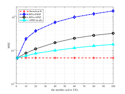
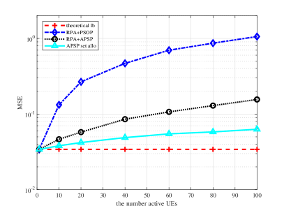
In Figure 3, we compare the MSE-CE performance of pilot assignment schemes and theoretical lower bound versus different numbers of active UEs. In the legend, we rewrite “lower bound” and “allocation” to “lb” and “allo” for short, respectively. Figure 3a and Figure 3b show the performance with Z=1Z=1 and Z=2Z=2 OFDM symbols used for pilot transmission in a slot, respectively. It is shown that the performance of each scheme is improved when more OFDM symbols are used for pilot transmission. For the PSOP-based RPA scheme, UEs are randomly assigned pilots from phase shift orthogonal pilot set. The number of PSOPs is ZNc/Ncp\lfloor ZN_{c}/N_{cp}\rfloor. It can cause serious pilot interference, since the number of PSOPs is far less than that of UEs. For the APSP-based RPA scheme, UEs are randomly assigned phase shifts from 𝚿\mathbf{\Psi}. It can utilize channel sparsity and outperform the PSOP-based scheme. Although the proposed APSP set allocation scheme is suboptimal in general compared with exhaustive search, substantial performance gains in terms of MSE-CE can still be achieved for different numbers of active UEs and pilot symbols. This is because it can reduce the overlap of angle-delay domain channel power distributions between the desired UE and interference with corresponding cyclic shifts in the delay domain. As observed from the trend of each curve, the performance gain of the proposed scheme can still be obvious when the number of active UEs is more than 100. Moreover, the theoretical lower bound is plotted, where each UE is assumed to be assigned a dedicated orthogonal pilot. As the number of active UEs increases, the MSE-CE of each pilot assignment scheme and the gap between it and corresponding lower bound increase.

Refer to caption
(a)
Refer to caption
(b)
Figure 3: Comparison of MSE-CE of pilot assignment schemes and theoretical lower bound with AP selection versus different numbers of active UEs assuming ζ=0.2μs\zeta\!=\!0.2~{}\mu\mathrm{s}, ς=2\varsigma\!=\!2^{\circ}, L=10L\!=\!10, and λ=0.7\lambda\!=\!0.7. (a) Results are shown with Z=1Z\!=\!1. (b) Results are shown with Z=2Z\!=\!2.

5.2.2 The MSE-CE Performance with Different Channel Sparsity

In Figure 4, we show the MSE-CE performance of pilot assignment schemes and lower bound versus different channel sparsity. In Figure 4a, performance comparisons are presented versus different angle spreads. Different delay spreads are considered in Figure 4b.

Refer to caption
(a)
Refer to caption
(b)
Figure 4: Comparison of MSE-CE of pilot assignment schemes and theoretical lower bound with AP selection versus channel sparsity with L=10\!L\!=\!10, Ka=50\!K_{a}\!=\!50, λ=0.7\!\lambda\!=\!0.7, and Z=1\!Z\!=\!1. (a) Results are given versus angle spreads with ζ=0.2μs\zeta\!=\!0.2~{}\!\mu\mathrm{s}. (b) Results are given versus delay spreads with ς=2\varsigma\!=\!2^{\circ}.

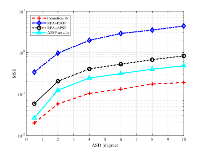
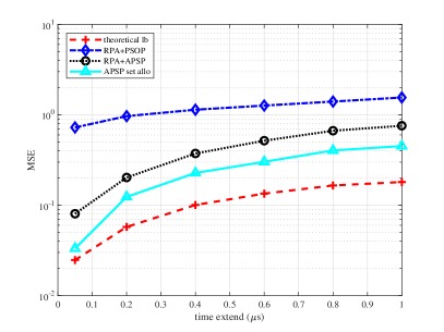
The APSP-based RPA scheme outperforms the scheme based on PSOP. If the APSP set allocation scheme is adopted, the performance can be further improved and close to its theoretical lower bound especially when the angle spread and delay spread are small. Besides, the performance of each scheme improves as angle spread or delay spread decreases, i.e., as channels become more sparse.

5.2.3 The MSE-CE Performance with Different Numbers of APs and Different AP Selection Coefficients

Figure 5 compares the MSE-CE cumulative distributions (CDFs) for pilot assignment schemes and lower bounds. In Figure 5a, MSE-CE CDFs are presented for different numbers of APs.

Refer to caption
(a)
Refer to caption
(b)
Figure 5: CDFs of MSE-CE for pilot assignment schemes and theoretical lower bounds with AP selection assuming Ka=50K_{a}\!=\!50, ζ=0.2μs\zeta\!=\!0.2~{}\!\mu\mathrm{s}, ς=2\varsigma\!=\!2^{\circ}, and Z=1Z=1. (a) Results are shown with λ=0.7\lambda\!=\!0.7 and L=15L\!=\!15 and 2020, respectively. (b) Results are shown with L=10L\!=\!10 and λ=0.8\lambda\!=\!0.8 and 0.90.9, respectively.

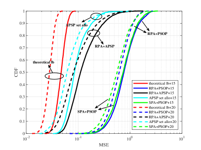
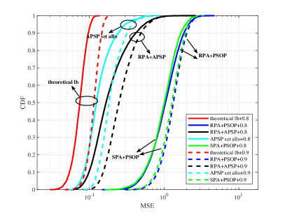
The performance of each scheme improves as the number of APs increases. This is because the macro-diversity provided by many APs reduces the risk that a UE has large distances to all APs. Figure 5b shows the MSE-CE CDFs of pilot assignment schemes with different AP selection coefficients. The performance of each scheme improves as λ\lambda decreases. This is because APs with better channel estimation performance for a UE are possible to have larger large-scale fading coefficients. When λ\lambda is increased, more APs far from a given UE are taken into account, and the MSE-CE averaged over serving APs of a UE can be worse. Besides, compared with the PSOP-based RPA scheme, the SPA scheme [18] has limited median gain in crowded scenarios. Owing to the reduced pilot interference effect, the performance of the proposed APSP set allocation scheme is close to the lower bound and significantly outperforms other schemes in both median and 95%-likely performance.

5.2.4 The SE Performance

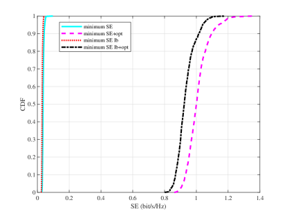
In Figure 6, we present the CDFs of the minimum SE and minimum SE lower bound among active UEs with and without power control under the APSP set allocation scheme. Based on Algorithm 2 with ϵ=0.02\epsilon=0.02, we maximize the minimum SE lower bound among KaK_{a} active UEs, which significantly outperforms the case without power control in both median and 95%-likely performance. Applying the optimized power coefficients of Problem (35) to the real minimum SE among active UEs, it is shown that power control can significantly benefit the minimum SE.

Refer to caption
Figure 6: CDFs of the minimum SE lower bound among active UEs and corresponding SE with and without power control under the proposed APSP set allocation scheme with Ka=50K_{a}=50, L=10L=10, λ=0.7\lambda=0.7, ζ=0.8μs\zeta=0.8~{}\mu\mathrm{s}, ς=8\varsigma=8^{\circ}, Z=1Z=1, and 50 taps.

6 Conclusion

In this paper, we considered uplink pilot and data transmission in crowded cell-free massive MIMO-OFDM systems with spatial and frequency correlation. For the pilot transmission, we utilized pilot phase shift hopping patterns to identify active UEs. Meanwhile, we derived a closed-form expression of MSE-CE with APSP, and provided an optimal condition of minimizing MSE-CE. According to this condition, we further developed an APSP set allocation scheme to reduce channel estimation error. This scheme is insensitive to the active pattern of UEs and does not need to be recomputed frequently. Besides, the expressions of SE and a lower bound of SE were derived. For the data transmission, we devised a max-min power control algorithm to maximize the minimum SE lower bound among active UEs. We can obtain the globally optimal solution of this problem by iteratively solving linear programs. Significant performance gains in terms of MSE-CE were observed for the proposed APSP set allocation scheme because it can fully utilize the channel sparsity. Compared with the equal power control, our proposed power allocation scheme can improve the minimum SE among active UEs in both median and 95%-likely performance. Hence, the proposed APSP set allocation scheme and the power control scheme are crucial and suitable for crowded cell-free massive MIMO-OFDM systems with frequently and spatially correlated channels.

Appendix A Proof of Proposition 1

From the definition of 𝐕N×N\mathbf{V}_{N\times N} in Proposition 1, we have

[𝐕N×NH𝐕N×N]i,j=1Nn=0N1exp{ȷ¯π(ji)(2nN1)}=Nδ(ji),\left[\mathbf{V}_{N\times N}^{H}\mathbf{V}_{N\times N}\right]_{i,j}=\frac{1}{N}\sum_{n=0}^{N-1}\exp\left\{-\overline{\jmath}\pi(j-i)\left(\frac{2n}{N}-1\right)\right\}\stackrel{{\scriptstyle{N\rightarrow\infty}}}{{=}}\delta(j-i), (38)

i.e., 𝐕N×NH𝐕N×N=N𝐈N×N\mathbf{V}_{N\times N}^{H}\mathbf{V}_{N\times N}\stackrel{{\scriptstyle N\rightarrow\infty}}{{=}}\mathbf{I}_{N\times N}. We have 𝐕M×MH𝐕M×M=(𝐈L×LH𝐈L×L)(𝐕N×NH𝐕N×N)=N𝐈M×M\mathbf{V}_{M\times M}^{H}\mathbf{V}_{M\times M}=\left(\mathbf{I}_{L\times L}^{H}\mathbf{I}_{L\times L}\right)\otimes\left(\mathbf{V}_{N\times N}^{H}\mathbf{V}_{N\times N}\right)\stackrel{{\scriptstyle N\rightarrow\infty}}{{=}}\mathbf{I}_{M\times M}.

From (1) and (2), we can obtain

vec{𝐆kβ}=q=0Ncp1π2π2[𝐟Nc,q𝐯M(θ)]𝐚MNc,kβ(θ,qTs)dθ,\operatorname{vec}\left\{\mathbf{G}_{k}^{\beta}\right\}=\sum_{q=0}^{N_{\rm{cp}}-1}\int_{-\frac{\pi}{2}}^{\frac{\pi}{2}}\left[\mathbf{f}_{N_{c},q}\otimes\mathbf{v}_{M}(\theta)\right]\odot\mathbf{a}_{MN_{c},k}^{\beta}\left(\theta,qT_{s}\right)\mathrm{d}\theta, (39)

where 𝐯M(θ)𝟏L×1𝐯N(θ)\mathbf{v}_{M}(\theta)\triangleq\mathbf{1}_{L\times 1}\otimes\mathbf{v}_{N}(\theta), 𝐟Nc,q[1exp{ȷ¯2π1Ncq}exp{ȷ¯2πNc1Ncq}]T\mathbf{f}_{N_{c},q}\triangleq\left[1\;\exp\left\{-\overline{\jmath}2\pi\frac{1}{N_{c}}q\right\}\!\;\cdots\!\;\exp\left\{-\overline{\jmath}2\pi\frac{N_{c}-1}{N_{c}}q\right\}\right]^{T}, 𝐚MNc,kβ(θ,qTs)𝟏Nc×1𝐚L,kβ(θ,qTs)𝟏N×1\mathbf{a}_{MN_{c},k}^{\beta}\left(\theta,qT_{s}\right)\triangleq\mathbf{1}_{N_{c}\times 1}\otimes\mathbf{a}^{\beta}_{L,k}(\theta,qT_{s})\otimes\mathbf{1}_{N\times 1}, and 𝐚L,kβ(θ,qTs)[ak,0β(θ,qTs)ak,1β(θ,qTs)ak,L1β(θ,qTs)]T\mathbf{a}^{\beta}_{L,k}(\theta,qT_{s})\triangleq\left[a_{k,0}^{\beta}(\theta,qT_{s})\!\;\;a_{k,1}^{\beta}(\theta,qT_{s})\cdots a_{k,L-1}^{\beta}(\theta,qT_{s})\right]^{T}. The space-frequency domain channel covariance matrix 𝐑kβ\mathbf{R}_{k}^{\beta} can be obtained as

𝐑kβ\displaystyle\mathbf{R}^{\beta}_{k} =𝔼{vec{𝐆kβ}vecH{𝐆kβ}}\displaystyle=\mathbb{E}\bigg{\{}\operatorname{vec}\left\{\mathbf{G}_{k}^{\beta}\right\}\operatorname{vec}^{H}\left\{\mathbf{G}_{k}^{\beta}\right\}\bigg{\}}
=q=0Ncp1π2π2q=0Ncp1π2π2[𝐟Nc,q𝐯M(θ)][𝐟Nc,q𝐯M(θ)]H𝔼{𝐚MNc,kβ(θ,qTs)(𝐚MNc,kβ(θ,qTs))H}dθdθ.\displaystyle=\sum_{q=0}^{N_{\rm{cp}}-1}\int_{-\frac{\pi}{2}}^{\frac{\pi}{2}}\sum_{q^{\prime}=0}^{N_{\rm{cp}}-1}\int_{-\frac{\pi}{2}}^{\frac{\pi}{2}}\left[\mathbf{f}_{N_{c},q}\otimes\mathbf{v}_{M}(\theta)\right]{\left[\mathbf{f}_{N_{c},q^{\prime}}\otimes\mathbf{v}_{M}(\theta^{\prime})\right]}^{H}\odot\mathbb{E}\left\{\mathbf{a}_{MN_{c},k}^{\beta}\left(\theta,qT_{s}\right){\left(\mathbf{a}_{MN_{c},k}^{\beta}\left(\theta^{\prime},q^{\prime}T_{s}\right)\right)}^{H}\right\}\mathrm{d}\theta\mathrm{d}\theta^{\prime}. (40)

Define Pk,lAD(θ,qTs)Pk,lA(θ)Pk,lD(qTs)P^{AD}_{k,l}(\theta,qT_{s})\triangleq P^{A}_{k,l}(\theta)P^{D}_{k,l}(qT_{s}). For an arbitrary non-negative integer d, let ndd/Mn_{d}\triangleq\lfloor d/M\rfloor, mddMm_{d}\triangleq\langle d\rangle_{M}, rmdmd/Nr_{m_{d}}\triangleq\lfloor m_{d}/N\rfloor, and smdmdNs_{m_{d}}\triangleq\langle m_{d}\rangle_{N}. We have

[𝐑kβ]i,j\displaystyle\left[\mathbf{R}^{\beta}_{k}\right]_{i,j} =q=0Ncp1π2π2q=0Ncp1π2π2[𝐟Nc,q𝐯M(θ)]i[𝐟Nc,q𝐯M(θ)]j𝔼{[𝐚MNc,kβ(θ,qTs)]i[𝐚MNc,kβ(θ,qTs)]j}dθdθ\displaystyle=\sum_{q=0}^{N_{\rm{cp}}-1}\int_{-\frac{\pi}{2}}^{\frac{\pi}{2}}\sum_{q^{\prime}=0}^{N_{\rm{cp}}-1}\int_{-\frac{\pi}{2}}^{\frac{\pi}{2}}\left[\mathbf{f}_{N_{c},q}\otimes\mathbf{v}_{M}(\theta)\right]_{i}{\left[\mathbf{f}_{N_{c},q^{\prime}}\otimes\mathbf{v}_{M}(\theta^{\prime})\right]}^{\ast}_{j}\mathbb{E}\left\{\left[\mathbf{a}_{MN_{c},k}^{\beta}\left(\theta,qT_{s}\right)\right]_{i}{\left[\mathbf{a}_{MN_{c},k}^{\beta}\left(\theta^{\prime},q^{\prime}T_{s}\right)\right]}^{\ast}_{j}\right\}\mathrm{d}\theta\mathrm{d}\theta^{\prime}
=(a)q=0Ncp1π2π2[𝐟Nc,q]ni[𝐟Nc,q]nj[𝐯N(θ)]smi[𝐯N(θ)]smj𝔼{ak,rmiβ(θ,qTs)(ak,rmjβ(θ,qTs))}dθ\displaystyle\stackrel{{\scriptstyle(\mathrm{a})}}{{=}}\sum_{q=0}^{N_{\rm{cp}}-1}\int_{-\frac{\pi}{2}}^{\frac{\pi}{2}}\left[\mathbf{f}_{N_{c},q}\right]_{n_{i}}\left[\mathbf{f}_{N_{c},q}\right]^{\ast}_{n_{j}}\left[\mathbf{v}_{N}(\theta)\right]_{s_{m_{i}}}\left[\mathbf{v}_{N}(\theta)\right]^{\ast}_{s_{m_{j}}}\mathbb{E}\left\{a_{k,r_{m_{i}}}^{\beta}\left(\theta,qT_{s}\right)\left(a_{k,r_{m_{j}}}^{\beta}\left(\theta,qT_{s}\right)\right)^{\ast}\right\}\mathrm{d}\theta
=q=0Ncp1π2π2exp{ȷ¯2πninjNcq}exp{ȷ¯π(smismj)sin(θ)}β(k,rmi)Pk,rmiAD(θ,qTs)δ(rmirmj)dθ,\displaystyle=\sum_{q=0}^{N_{\rm{cp}}-1}\int_{-\frac{\pi}{2}}^{\frac{\pi}{2}}\exp\left\{-\overline{\jmath}2\pi\frac{n_{i}-n_{j}}{N_{\mathrm{c}}}q\right\}\exp\left\{-\overline{\jmath}\pi\left(s_{m_{i}}-s_{m_{j}}\right)\sin(\theta)\right\}\beta\left(k,r_{m_{i}}\right)P^{AD}_{k,r_{m_{i}}}(\theta,qT_{s})\delta\left(r_{m_{i}}-r_{m_{j}}\right)\mathrm{d}\theta, (41)

where (a) follows from [𝐀𝐁]i,j=[𝐀]ni,nj[𝐁]mi,mj[\mathbf{A}\otimes\mathbf{B}]_{i,j}=[\mathbf{A}]_{n_{i},n_{j}}[\mathbf{B}]_{m_{i},m_{j}} for matrices 𝐀\mathbf{A} and 𝐁\mathbf{B}. Meanwhile, we have

[(𝐅Nc×Ncp𝐕M×M)diag{vec{𝚼kβ}}(𝐅Nc×Ncp𝐕M×M)H]i,j\displaystyle\;\;\;\;\left[\left(\mathbf{F}_{N_{c}\times N_{\mathrm{cp}}}\otimes\mathbf{V}_{M\times M}\right)\operatorname{diag}\left\{\operatorname{vec}\left\{\bm{\Upsilon}_{k}^{\beta}\right\}\right\}\left(\mathbf{F}_{N_{c}\times N_{\mathrm{cp}}}\otimes\mathbf{V}_{M\times M}\right)^{H}\right]_{i,j}
=d=0MNcp1[vec{𝚼kβ}]d[(𝐅Nc×Ncp𝐕M×M)]i,d[(𝐅Nc×Ncp𝐕M×M)]j,d\displaystyle=\sum_{d=0}^{MN_{\mathrm{cp}}-1}\left[\operatorname{vec}\left\{\bm{\Upsilon}_{k}^{\beta}\right\}\right]_{d}\left[\left(\mathbf{F}_{N_{c}\times N_{\mathrm{cp}}}\otimes\mathbf{V}_{M\times M}\right)\right]_{i,d}\left[\left(\mathbf{F}_{N_{c}\times N_{\mathrm{cp}}}\otimes\mathbf{V}_{M\times M}\right)\right]_{j,d}^{\ast}
=nd=0Ncp1md=rmirmi+N1[𝚼k,rmdβ]smd,nd[𝐅Nc×Ncp]ni,nd[𝐅Nc×Ncp]nj,nd[𝐕N×N]smi,smd[𝐕N×N]smj,smdδ(rmirmj)\displaystyle=\sum_{n_{d}=0}^{N_{\mathrm{cp}}-1}\sum_{m_{d}=r_{m_{i}}}^{r_{m_{i}}+N-1}\left[\bm{\Upsilon}_{k,r_{m_{d}}}^{\beta}\right]_{s_{m_{d}},n_{d}}\left[\mathbf{F}_{N_{c}\times N_{\mathrm{cp}}}\right]_{n_{i},n_{d}}\left[\mathbf{F}_{N_{c}\times N_{\mathrm{cp}}}\right]_{n_{j},n_{d}}^{\ast}\left[\mathbf{V}_{N\times N}\right]_{s_{m_{i}},s_{m_{d}}}\left[\mathbf{V}_{N\times N}\right]_{s_{m_{j}},s_{m_{d}}}^{\ast}\delta\left(r_{m_{i}}-r_{m_{j}}\right)
=nd=0Ncp1md=0N1β(k,rmi)(θmd+1θmd)Pk,rmiAD(θmd,ndTs)exp{ȷ¯2πninjNcnd}exp{ȷ¯π(smismj)sin(θmd)}δ(rmirmj)\displaystyle=\sum_{n_{d}=0}^{N_{\mathrm{cp}}-1}\!\sum_{m_{d}=0}^{N-1}\beta\!\left(k,r_{m_{i}}\right)\left(\theta_{m_{d}+1}\!-\!\theta_{m_{d}}\right)P^{AD}_{k,r_{m_{i}}}\!(\theta_{m_{d}},n_{d}T_{s})\exp\left\{-\overline{\jmath}2\pi\frac{n_{i}\!-\!n_{j}}{N_{\mathrm{c}}}n_{d}\right\}\exp\left\{-\overline{\jmath}\pi\left(\!s_{m_{i}}\!\!-\!s_{m_{j}}\!\right)\sin\left(\theta_{m_{d}}\right)\right\}\delta\!\left(\!r_{m_{i}}\!\!-\!r_{m_{j}}\!\right)
=Nq=0Ncp1π2π2β(k,rmi)Pk,rmiAD(θ,qTs)exp{ȷ¯2πninjNcq}exp{ȷ¯π(smismj)sin(θ)}δ(rmirmj)dθ.\displaystyle\stackrel{{\scriptstyle{N\rightarrow\infty}}}{{=}}\sum_{q=0}^{N_{\mathrm{cp}}-1}\int_{-\frac{\pi}{2}}^{\frac{\pi}{2}}\beta\left(k,r_{m_{i}}\right)P^{AD}_{k,r_{m_{i}}}(\theta,qT_{s})\exp\left\{-\overline{\jmath}2\pi\frac{n_{i}-n_{j}}{N_{\mathrm{c}}}q\right\}\exp\left\{-\overline{\jmath}\pi\left(s_{m_{i}}-s_{m_{j}}\right)\sin(\theta)\right\}\delta\left(r_{m_{i}}-r_{m_{j}}\right)\mathrm{d}{\theta}. (42)

Since the power angle-delay spectrum is bounded [24], the limit in the first equation of (A) exists. Since (A) is equal to (A), 𝐑kβ\mathbf{R}_{k}^{\beta} can be obtained as (8). The proof of (9) is given by

𝐑kβ\displaystyle\mathbf{R}^{\beta}_{k} =N(a)(𝐅Nc×Ncp𝐕M×M)𝔼{vec{𝐇kβ}vecH{𝐇kβ}}(𝐅Nc×Ncp𝐕M×M)H\displaystyle\stackrel{{\scriptstyle\stackrel{{\scriptstyle(a)}}{{N\rightarrow\infty}}}}{{=}}\left(\mathbf{F}_{N_{c}\times N_{\mathrm{cp}}}\otimes\mathbf{V}_{M\times M}\right)\mathbb{E}\left\{\operatorname{vec}\left\{\mathbf{H}_{k}^{\beta}\right\}\operatorname{vec}^{H}\left\{\mathbf{H}_{k}^{\beta}\right\}\right\}\left(\mathbf{F}_{N_{c}\times N_{\mathrm{cp}}}\otimes\mathbf{V}_{M\times M}\right)^{H}
=(b)𝔼{vec{𝐕M×M𝐇kβ𝐅Nc×NcpH}vecH{𝐕M×M𝐇kβ𝐅Nc×NcpH}},\displaystyle\;\;\stackrel{{\scriptstyle(b)}}{{=}}\mathbb{E}\left\{\operatorname{vec}\left\{\mathbf{V}_{M\times M}\mathbf{H}_{k}^{\beta}\;\mathbf{F}^{H}_{N_{c}\times N_{\mathrm{cp}}}\right\}\operatorname{vec}^{H}\left\{\mathbf{V}_{M\times M}\mathbf{H}_{k}^{\beta}\;\mathbf{F}^{H}_{N_{c}\times N_{\mathrm{cp}}}\right\}\right\}, (43)

where (a) follows from (6) and (8), and (b) follows from the fact that (𝐂T𝐀)vec{𝐁}=vec{𝐀𝐁𝐂}\left(\mathbf{C}^{T}\otimes\mathbf{A}\right)\operatorname{vec}\left\{\mathbf{B}\right\}=\operatorname{vec}\left\{\mathbf{ABC}\right\}. Besides, since 𝐑kβ=𝔼{vec{𝐆kβ}vecH{𝐆kβ}}\mathbf{R}^{\beta}_{k}=\mathbb{E}\left\{\operatorname{vec}\left\{\mathbf{G}_{k}^{\beta}\right\}\operatorname{vec}^{H}\left\{\mathbf{G}_{k}^{\beta}\right\}\right\}, we can obtain (9).

Appendix B Proof of Proposition 2

Considering the non-negative property of the angle-delay domain channel power distribution, it is satisfied that in (19) the term R𝒦ai,j,p,m,q=[𝚼𝒦ai,jβ,0]m,q[𝚼𝒦ai,jβ]m,q+jjj=0Ka1δ(𝒫i,jpZ𝒫i,jpZ)[𝚼𝒦ai,jβ,𝒫i,jp/Z𝒫i,jp/Z]m,q+1ρpZ[0,1)R_{\mathcal{K}_{a}^{i,j},p,m,q}=\frac{{{\left[\mathbf{\Upsilon}_{\mathcal{K}_{a}^{i,j}}^{\beta,0}\right]}_{m,q}}}{{{\left[\mathbf{\Upsilon}_{\mathcal{K}_{a}^{i,j}}^{\beta}\right]}_{m,q}}+\sum\limits_{\stackrel{{\scriptstyle j^{\prime}=0}}{{j^{\prime}\neq j}}}^{K_{a}-1}\delta\left(\left\langle\mathcal{P}_{i,j^{\prime}}^{p}\right\rangle_{Z}-\left\langle\mathcal{P}_{i,j}^{p}\right\rangle_{Z}\right){{{\left[\mathbf{\Upsilon}_{\mathcal{K}_{a}^{i,{j}^{\prime}}}^{\beta,\left\lfloor{\mathcal{P}_{i,j^{\prime}}^{p}}/{Z}\right\rfloor-\left\lfloor{\mathcal{P}_{i,j}^{p}}/{Z}\right\rfloor}\right]}_{m,q}}}+\frac{1}{{{\rho}_{p}}Z}}\in[0,1). Then, we have ε𝒦ai,j,p,m,q0=[𝚼𝒦ai,j0]m,q(1R𝒦ai,j,p,m,q)0\varepsilon_{\mathcal{K}_{a}^{i,j},p,m,q}^{0}={{\left[\mathbf{\Upsilon}^{0}_{\mathcal{K}_{a}^{i,j}}\right]}_{m,q}}\left(1-R_{\mathcal{K}_{a}^{i,j},p,m,q}\right)\geq 0. When [𝚼𝒦ai,j0]m,q=0{{\left[\mathbf{\Upsilon}^{0}_{\mathcal{K}_{a}^{i,j}}\right]}_{m,q}}=0, ε𝒦ai,j,p,m,q0\varepsilon_{\mathcal{K}_{a}^{i,j},p,m,q}^{0} can achieve the minimum value 0; when [𝚼𝒦ai,j0]m,q>0{{\left[\mathbf{\Upsilon}^{0}_{\mathcal{K}_{a}^{i,j}}\right]}_{m,q}}>0, ε𝒦ai,j,p,m,q0\varepsilon_{\mathcal{K}_{a}^{i,j}\!,p,m,q}^{0} can be minimized if and only if R𝒦ai,j,p,m,qR_{\mathcal{K}_{a}^{i,j}\!,p,m,q} is maximized, i.e., jjj=0Ka1δ(𝒫i,jpZ𝒫i,jpZ)[𝚼𝒦ai,jβ,𝒫i,jp/Z𝒫i,jp/Z]m,q=0\sum\limits_{\stackrel{{\scriptstyle j^{\prime}=0}}{{j^{\prime}\neq j}}}^{K_{a}-1}\!\delta\!\left(\left\langle\mathcal{P}_{i,j^{\prime}}^{p}\!\right\rangle_{\!Z}\!\!-\!\left\langle\mathcal{P}_{i,j}^{p}\right\rangle_{\!Z}\right){{{\!\left[\!\mathbf{\Upsilon}_{\mathcal{K}_{a}^{i,{j}^{\prime}}}^{\beta,\left\lfloor{\mathcal{P}_{i,j^{\prime}}^{p}}\!/{Z}\right\rfloor-\left\lfloor{\mathcal{P}_{i,j}^{p}}/{Z}\right\rfloor}\right]}_{m,q}}}\!=0. Hence, we can conclude the minimum condition of ε𝒦ai,j,p,m,q0\varepsilon_{\mathcal{K}_{a}^{i,j},p,m,q}^{0} as [𝚼𝒦ai,j0]m,q[𝚼𝒦ai,j0]m,q[𝚼𝒦ai,jβ,𝒫i,jp/Z𝒫i,jp/Z]m,q=0{{\left[\mathbf{\Upsilon}^{0}_{\mathcal{K}_{a}^{i,j}}\right]}_{m,q}}{{\left[\mathbf{\Upsilon}^{0}_{\mathcal{K}_{a}^{i,j}}\right]}_{m,q}}{{{\left[\mathbf{\Upsilon}_{\mathcal{K}_{a}^{i,{j}^{\prime}}}^{\beta,\left\lfloor{\mathcal{P}_{i,j^{\prime}}^{p}}/{Z}\right\rfloor-\left\lfloor{\mathcal{P}_{i,j}^{p}}/{Z}\right\rfloor}\right]}_{m,q}}}=0 for 𝒫i,jpZ=𝒫i,jpZ\left\langle\mathcal{P}_{i,j^{\prime}}^{p}\right\rangle_{Z}=\left\langle\mathcal{P}_{i,j}^{p}\right\rangle_{Z}, j=0,1,,Ka1j^{\prime}=0,1,\cdots,K_{a}-1, and jjj^{\prime}\neq j.

For any choice of i,j,p,m,andqi,j,p,m,\text{and}\;q, ε𝒦ai,j,p,m,q0\varepsilon_{\mathcal{K}_{a}^{i,j},p,m,q}^{0} should be minimized. The optimal condition can be expressed as 𝚼k0𝚼k0𝚼kβ,ϕk/Zϕk/Z=𝟎\mathbf{\Upsilon}^{0}_{k}\odot\mathbf{\Upsilon}^{0}_{k}\odot\mathbf{\Upsilon}_{{{k}^{\prime}}}^{\beta,\left\lfloor{{\phi}_{{{k}^{\prime}}}}/Z\right\rfloor-\left\lfloor{{\phi}_{{{k}}}}/Z\right\rfloor}=\mathbf{0} for ϕkZ=ϕkZ\left\langle{{\phi}_{{{k}^{\prime}}}}\right\rangle_{Z}=\left\langle{{\phi}_{{{k}}}}\right\rangle_{Z}, k𝒦k^{\prime}\in\mathcal{K}, and kkk\neq k^{\prime}. It is a necessary and sufficient condition, but it can be expressed as other forms. The reason why we choose 𝚼k0𝚼k0𝚼kβ,ϕk/Zϕk/Z\mathbf{\Upsilon}_{k}^{0}\odot\mathbf{\Upsilon}_{k}^{0}\odot\mathbf{\Upsilon}_{{{k}^{\prime}}}^{\beta,\left\lfloor{{\phi}_{{{k}^{\prime}}}}/Z\right\rfloor-\left\lfloor{{\phi}_{{{k}}}}/Z\right\rfloor} but not 𝚼k0𝚼kβ,ϕk/Zϕk/Z\mathbf{\Upsilon}_{k}^{0}\odot\mathbf{\Upsilon}_{{{k}^{\prime}}}^{\beta,\left\lfloor{{\phi}_{{{k}^{\prime}}}}/Z\right\rfloor-\left\lfloor{{\phi}_{{{k}}}}/Z\right\rfloor} is because we want to make the interference 𝚼kβ,ϕk/Zϕk/Z\mathbf{\Upsilon}_{{{k}^{\prime}}}^{\beta,\left\lfloor{{\phi}_{{{k}^{\prime}}}}/Z\right\rfloor-\left\lfloor{{\phi}_{{{k}}}}/Z\right\rfloor} smaller when 𝚼k0\mathbf{\Upsilon}_{k}^{0} is large. In this way, ε¯0{{{\overline{\varepsilon}}}^{0}} can be smaller.

Based on (19) and (20), we can obtain

𝔼𝒰,𝒦a,𝒫(ε0)\displaystyle{{\mathbb{E}}_{\mathcal{U},{{\mathcal{K}}_{{a}}},\mathcal{P}}}(\varepsilon^{0}) =i=0N𝒦a1j=0Ka1p=0Nϕ11N𝒦aKaNϕNc|𝒦ai,j|m=0M1q=0Ncp1{ε𝒦ai,j,p,m,q0}\displaystyle=\sum\limits_{i=0}^{{{N}_{{{\mathcal{K}}_{a}}}-1}}{\sum\limits_{j=0}^{{{K}_{a}-1}}{\sum\limits_{p=0}^{{{N}_{\phi}-1}}{\frac{1}{{{N}_{{{\mathcal{K}}_{a}}}}{{K}_{a}}{{N}_{\phi}}{{N}_{c}}{\left|\mathcal{B}_{{\mathcal{K}}^{i,j}_{a}}\right|}}}{\sum\limits_{m=0}^{M-1}{\sum\limits_{q=0}^{{{N}_{\mathrm{cp}}}-1}{\left\{\varepsilon_{\mathcal{K}_{a}^{i,j},p,m,q}^{0}\right\}}}}}}
i=0N𝒦a1j=0Ka1p=0Nϕ11N𝒦aKaNϕNc|𝒦ai,j|m=0M1q=0Ncp1{[𝚼𝒦ai,j0]m,q[𝚼𝒦ai,j0]m,q[𝚼𝒦ai,jβ,0]m,q[𝚼𝒦ai,jβ]m,q+1ρpZ}\displaystyle{\geq}\sum\limits_{i=0}^{{{N}_{{{\mathcal{K}}_{a}}}-1}}{\sum\limits_{j=0}^{{{K}_{a}-1}}{\sum\limits_{p=0}^{{{N}_{\phi}-1}}{\frac{1}{{{N}_{{{\mathcal{K}}_{a}}}}{{K}_{a}}{{N}_{\phi}}{{N}_{c}}{\left|\mathcal{B}_{{\mathcal{K}}^{i,j}_{a}}\right|}}}{\sum\limits_{m=0}^{M-1}{\sum\limits_{q=0}^{{{N}_{\mathrm{cp}}}-1}{\left\{{{\left[\mathbf{\Upsilon}^{0}_{\mathcal{K}_{a}^{i,j}}\right]}_{m,q}}-\frac{{{\left[\mathbf{\Upsilon}^{0}_{\mathcal{K}_{a}^{i,j}}\right]}_{m,q}}{{\left[\mathbf{\Upsilon}_{\mathcal{K}_{a}^{i,j}}^{\beta,0}\right]}_{m,q}}}{{{\left[\mathbf{\Upsilon}_{\mathcal{K}_{a}^{i,j}}^{\beta}\right]}_{m,q}}+\frac{1}{{{\rho}_{p}}Z}}\right\}}}}}}
=(a)k=0K11KNc|k|m=0M1q=0Ncp1{[𝚼k0]m,q[𝚼k0]m,q[𝚼kβ,0]m,q[𝚼kβ]m,q+1ρpZ}\displaystyle\stackrel{{\scriptstyle(\mathrm{a})}}{{=}}{\sum\limits_{k=0}^{{K-1}}{\frac{1}{K{{N}_{c}}{\left|\mathcal{B}_{k}\right|}}}{\sum\limits_{m=0}^{M-1}{\sum\limits_{q=0}^{{{N}_{\mathrm{cp}}}-1}{\left\{{{\left[\mathbf{\Upsilon}^{0}_{k}\right]}_{m,q}}-\frac{{{\left[\mathbf{\Upsilon}^{0}_{k}\right]}_{m,q}}{{\left[\mathbf{\Upsilon}_{k}^{\beta,0}\right]}_{m,q}}}{{{\left[\mathbf{\Upsilon}_{k}^{\beta}\right]}_{m,q}}+\frac{1}{{{\rho}_{p}Z}}}\right\}}}}}
=[𝔼𝒰,𝒦a,𝒫(ε0)]min,\displaystyle=\left[{{{\mathbb{E}}_{\mathcal{U},{{\mathcal{K}}_{a}},\mathcal{P}}}(\varepsilon^{0})}\right]_{\min}, (44)

where (a) follows from the fact that when ε𝒦ai,j,p,m,q0\varepsilon_{\mathcal{K}_{a}^{i,j},p,m,q}^{0} is minimized, i.e., when the effect of pilot interference is eliminated, the average operation accounting for all possible active patterns and all types of phase shift selection is the same as the average operation over KK UEs in the network [11]. Then, we have ε¯min0=Ka=1Kp(Ka|K)[𝔼𝒰,𝒦a,𝒫(ε0)]min\overline{\varepsilon}^{0}_{\min}=\sum\limits_{K_{a}=1}^{K}{p(K_{a}|K)\left[{{{\mathbb{E}}_{\mathcal{U},{{\mathcal{K}}_{a}},\mathcal{P}}}(\varepsilon^{0})}\right]_{\min}}.

Appendix C Derivation of (30)

We can rewrite (29) as

rk,s=l=0L1νk,lrk,l,s=ρuηk𝔼{(𝐜k,sβ,0)H𝐠k,sβ}xk,s+Infsum,{{r}_{k,s}}=\sum\limits_{l=0}^{L-1}{\nu_{k,l}{{r}_{k,l,s}}}=\sqrt{{{\rho}_{u}}}\sqrt{{{\eta}_{k}}}\;\mathbb{E}\left\{\left(\mathbf{c}_{k,s}^{\beta,0}\right)^{H}{\mathbf{g}}_{k,s}^{\beta}\right\}{{x}_{k,s}}+\text{Inf}_{\text{sum}}^{\;{}^{\prime}}, (45)

where the interference term is given by

Infsum=ρuηk((𝐜k,sβ,0)H𝐠k,sβ𝔼{(𝐜k,sβ,0)H𝐠k,sβ})xk,s+ρuk𝒰𝒦ai\{k}ηk(𝐜k,sβ,0)H𝐠k,sβxk,s+(𝐜k,sβ,0)H𝐰s.\text{Inf}_{\text{sum}}^{\;{}^{\prime}}=\sqrt{{{\rho}_{u}}{{\eta}_{k}}}\left(\left(\mathbf{c}_{k,s}^{\beta,0}\right)^{H}{\mathbf{g}}_{k,s}^{\beta}-\mathbb{E}\left\{\left(\mathbf{c}_{k,s}^{\beta,0}\right)^{H}{\mathbf{g}}_{k,s}^{\beta}\right\}\right){{x}_{k,s}}+\sqrt{{{\rho}_{u}}}\sum\limits_{{k}^{\prime}\in\;\mathcal{U}_{\mathcal{K}_{a}}^{i}\backslash\left\{k\right\}}{\sqrt{{{\eta}_{{{k}^{\prime}}}}}\left(\mathbf{c}_{k,s}^{\beta,0}\right)^{H}\mathbf{g}_{{k}^{\prime},s}^{\beta}{{x}_{{k}^{\prime},s}}}+\left(\mathbf{c}_{k,s}^{\beta,0}\right)^{H}{{\mathbf{w}}_{s}}. (46)

We have 𝔼{Infsum}=0\mathbb{E}\left\{\text{Inf}_{\text{sum}}^{\;{}^{\prime}}\right\}=0. Since the transmitted signal of UE k is independent of the signals of other UEs and receiver noise, the interference is uncorrelated with the transmitted signal, i.e.,

𝔼{xk,sInfsum}=ρuηk𝔼{(𝐜k,sβ,0)H𝐠k,sβ𝔼{(𝐜k,sβ,0)H𝐠k,sβ}}𝔼{|xk,s|2}=0.\mathbb{E}\left\{x_{k,s}^{\ast}\text{Inf}_{\text{sum}}^{\;{}^{\prime}}\right\}=\sqrt{{{\rho}_{u}}}\sqrt{{{\eta}_{k}}}\;\mathbb{E}\left\{\left(\mathbf{c}_{k,s}^{\beta,0}\right)^{H}{\mathbf{g}}_{k,s}^{\beta}-\mathbb{E}\left\{\left(\mathbf{c}_{k,s}^{\beta,0}\right)^{H}{\mathbf{g}}_{k,s}^{\beta}\right\}\right\}\mathbb{E}\left\{|{{x}_{k,s}}|^{2}\right\}=0. (47)

The variance of the interference term is represented as

𝔼{|Infsum|2}=ρuk𝒰𝒦aiηk𝔼{|(𝐜k,sβ,0)H𝐠k,sβ|2}ρuηk|𝔼{(𝐜k,sβ,0)H𝐠k,sβ}|2+𝔼{𝐜k,sβ,02}.\mathbb{E}\left\{{{\left|\text{Inf}_{\text{sum}}^{\;{}^{\prime}}\right|}^{2}}\right\}={{\rho}_{u}}\sum\limits_{{k}^{\prime}\in\mathcal{U}^{i}_{{\mathcal{K}}_{a}}}{{{\eta}_{{{k}^{\prime}}}}\mathbb{E}\left\{{{\left|\left(\mathbf{c}_{k,s}^{\beta,0}\right)^{H}\mathbf{g}_{{k}^{\prime},s}^{\beta}\right|}^{2}}\right\}}-{{\rho}_{u}}{{\eta}_{k}}\left|\mathbb{E}\left\{{{\left(\mathbf{c}_{k,s}^{\beta,0}\right)^{H}{\mathbf{g}}_{k,s}^{\beta}}}\right\}\right|^{2}+\mathbb{E}\left\{\left\|\mathbf{c}_{k,s}^{\beta,0}\right\|^{2}\right\}. (48)

It follows from the independence between each of the zero-mean transmitted signals and the independence between signals and channels. Taking the OFDM CP overhead and pilot overhead into account, according to Corollary 1.3 in [33], we can obtain the SE lower bound as shown in (30).

\Acknowledgements

The work of Y. Wu was supported in part by the National Key R&D Program of China under Grant 2018YFB1801102, JiangXi Key R&D Program under Grant 20181ACE50028, National Science Foundation (NSFC) under Grant 61701301, the open research project of State Key Laboratory of Integrated Services Networks (Xidian University) under Grant ISN20-03, and Shanghai Key Laboratory of Digital Media Processing and Transmission (STCSM18DZ2270700). The work of Y. Wang was supported by the National Natural Science Foundation of China (No.61931019). The work of W. Zhang was supported by Shanghai Key Laboratory of Digital Media Processing and Transmission (STCSM18DZ2270700).

References

  • [1] Larsson E G, Edfors O, Tufvesson F, et al. Massive MIMO for next generation wireless systems. IEEE Commun Mag, 2014, 52: 186–195.
  • [2] Lu L, Li G Y, Swindlehurst A L, et al. An overview of massive MIMO: Benefits and challenges. IEEE J Sel Topics Signal Process, 2014, 8: 742–758.
  • [3] Ngo H Q, Ashikhmin A, Yang H, et al. Cell-free massive MIMO versus small cells. IEEE Trans Wireless Commun, 2017, 16: 1834–1850.
  • [4] Zhang J, Björnson E, Matthaiou M, et al. Prospective multiple antenna technologies for beyond 5G. to appear in IEEE J Sel Areas Commun, 2020.
  • [5] Zhang J, Chen S, Lin Y, et al. Cell-free massive MIMO: A new next-generation paradigm. IEEE Access, 2019, 7: 99878–99888.
  • [6] Cimini L J. Analysis and simulation of a digital mobile channel using orthogonal frequency division multiplexing. IEEE Trans Commun, 1985, 33: 665–675.
  • [7] Zhao J, Ni S, Yang L, et al. Multiband cooperation for 5G HetNets: A promising network paradigm. IEEE Veh Technol Mag, 2019, 14: 85–93.
  • [8] Bockelmann C, Pratas N, Nikopour H, et al. Massive machine-type communications in 5G: Physical and MAC-layer solutions. IEEE Commun Mag, 2016, 54: 59–65.
  • [9] Carvalho E de, Björnson E, Sørensen J H, et al. Random access protocols for massive MIMO. IEEE Commun Mag, 2017, 55: 216–222.
  • [10] Wu Y, Gao X, Zhou S, et al. Massive access for future wireless communication systems. to appear in IEEE Wireless Commun, 2020.
  • [11] Carvalho E de, Björnson E, Sørensen J H, et al. Random pilot and data access in massive MIMO for machine-type communications. IEEE Trans Wireless Commun, 2017, 16: 7703–7717.
  • [12] Chen Z, and Björnson E. Channel hardening and favorable propagation in cell-free massive MIMO with stochastic geometry. IEEE Trans Commun, 2018, 66: 5205–5219.
  • [13] Nayebi E, Ashikhmin A, Marzetta T L, et al. Precoding and power optimization in cell-free massive MIMO systems. IEEE Trans Wireless Commun, 2017, 16: 4445–4459.
  • [14] Yang H, and Marzetta T L. Energy efficiency of massive MIMO: Cell-free vs. cellular. Proc IEEE Veh Technol Conf (VTC Spring), Porto, 2018, 1–5.
  • [15] Björnson E, and Sanguinetti L. Making cell-free massive MIMO competitive with MMSE processing and centralized implementation. IEEE Trans Wireless Commun, 2020, 19: 77–90.
  • [16] Ngo H Q, Tran L, Duong T Q, et al. On the total energy efficiency of cell-free massive MIMO. IEEE Trans Green Commun Netw, 2018, 2: 25–39.
  • [17] Interdonato G, Björnson E, Ngo H Q, et al. Ubiquitous cell-free massive MIMO communications. Eurasip J Wireless Commun Netw, 2019.
  • [18] Attarifar M, Abbasfar A, and Lozano A. Random vs structured pilot assignment in cell-free massive MIMO wireless networks. Proc IEEE Int Conf on Commun (ICC), Kansas City, US, 2018, 1–6.
  • [19] Liu H, Zhang J, Zhang X, et al. Tabu-search-based pilot assignment for cell-free massive MIMO systems. IEEE Trans Veh Technol, 2020, 69: 2286–2290.
  • [20] Liu H, Zhang J, Jin S, et al. Graph coloring based pilot assignment for cell-free massive MIMO systems. IEEE Trans Veh Technol, 2020, 69: 9180–9184.
  • [21] Liu K, Raghavan V, and Sayeed A M. Capacity scaling and spectral efficiency in wide-band correlated MIMO channels. IEEE Trans Inf Theory, 2003, 49: 2504–2526.
  • [22] Adhikary A, Nam J, Ahn J Y, et al. Joint spatial division and multiplexing-The large-scale array regime. IEEE Trans Inf Theory, 2013, 59: 6441–6463.
  • [23] Fleury B H. First- and second-order characterization of direction dispersion and space selectivity in the radio channel. IEEE Trans Inf Theory, 2000, 46: 2027–2044.
  • [24] You L, Gao X, Swindlehurst A L, et al. Channel acquisition for massive MIMO-OFDM with adjustable phase shift pilots. IEEE Trans Signal Process, 2016, 64: 1461–1476.
  • [25] Pedersen K I, Mogensen P E, and Fleury B H. A stochastic model of the temporal and azimuthal dispersion seen at the base station in outdoor propagation environments. IEEE Trans Veh Technol, 2000, 49: 437–447.
  • [26] Tse D, and Viswanath P. Fundamentals of Wireless Communication. Cambridge: Cambridge University Press, 2005.
  • [27] You L, Gao X Q, Xia X G, et al. Pilot reuse for massive MIMO transmission over spatially correlated Rayleigh fading channels. IEEE Trans Wireless Commun, 2015, 14: 3352–3366.
  • [28] Wen C K, Jin S, Wong K K, et al. Channel estimation for massive MIMO using Gaussian-mixture Bayesian learning. IEEE Trans Wireless Commun, 2015, 14: 1356–1368.
  • [29] Li Y G. Simplified channel estimation for OFDM systems with multiple transmit antennas. IEEE Trans Wireless Commun, 2002, 1: 67–75.
  • [30] Björnson E, Jalde´\acute{\text{e}}n N, Bengtsson M, et al. Optimality properties, distributed strategies, and measurement-based evaluation of coordinated multicell OFDMA transmission. IEEE Trans Signal Process, 2011, 59: 6086–6101.
  • [31] Hartigan J A, and Wong M A. Algorithm AS 136: A k-means clustering algorithm. J R Stat Soc C-Appl, 1979, 28: 100–108.
  • [32] Marzetta T L, Larsson E G, Yang H, et al. Fundamentals of Massive MIMO. Cambridge: Cambridge University Press, 2016.
  • [33] Björnson E, Hoydis J, and Sanguinetti L. Massive MIMO networks: Spectral, energy, and hardware efficiency. Found Trends Signal Process, 2017, 11: 154–655.
  • [34] Schaible S. Fractional programming. II, on Dinkelbach’s Algorithm. Manage Sci, 1976, 22: 868–873.
  • [35] Karmarkar N K. A new polynomial-time algorithm for linear programming. Combinatorica, 1984, 4: 373–395.
  • [36] Björnson E, Sanguinetti L, Hoydis J, et al. Optimal design of energy-efficient multi-user MIMO systems: Is massive MIMO the answer? IEEE Trans Wireless Commun, 2015, 14: 3059–3075.
  • [37] Tang A, Sun J, and Gong K. Mobile propagation loss with a low base station antenna for NLOS street microcells in urban area. Proc IEEE Veh Technol Conf (VTC), 2001, 5: 333–336.