Using asteroseismology to characterise exoplanet host stars
Abstract
The last decade has seen a revolution in the field of asteroseismology – the study of stellar pulsations. It has become a powerful method to precisely characterise exoplanet host stars, and as a consequence also the exoplanets themselves. This synergy between asteroseismology and exoplanet science has flourished in large part due to space missions such as Kepler, which have provided high-quality data that can be used for both types of studies. Perhaps the primary contribution from asteroseismology to the research on transiting exoplanets is the determination of very precise stellar radii that translate into precise planetary radii, but asteroseismology has also proven useful in constraining eccentricities of exoplanets as well as the dynamical architecture of planetary systems. In this chapter, we introduce some basic principles of asteroseismology and review current synergies between the two fields.
1 Introduction
”You only know your planet as well as you know your star”. This could be the beginning of a sales pitch for asteroseismology – the study of stellar pulsations – as an important tool for exoplanet scientists to gain valuable information about their planets and planetary systems. This is because one of the strengths of asteroseismology is the ability to determine very precise stellar radii that can in turn be used to calculate the planetary size which, from the transit light curve, is known only as a function of the stellar size. Asteroseismology can also yield, for instance, the stellar age and luminosity, parameters that are important in order to assess the habitability of other planets.
Over the last decade, the field of asteroseismology has been revolutionised by space-based photometry provided by missions such as CoRoT and Kepler. Before the success of these missions, asteroseimic studies of even a single star were time-consuming and had only been carried out for a few targets (e.g. Cen A, Bouchy and Carrier 2001; Bedding et al. 2004). Today, oscillations have been detected in over 500 solar-type stars (Chaplin et al. 2014), a significant fraction of which are exoplanet host stars.
In this chapter we will introduce the basic principles of asteroseismology, describe how stellar properties can be derived from this and discuss the resulting precision. Hereafter we will focus on the synergy between asteroseismology and exoplanet science by highlighting how the fields combine and benefit from each other through some specific examples (see also Huber 2018).
2 Introduction to asteroseismology
Many different types of stars have been found to oscillate due to standing waves in their interiors. These oscillations give rise to detectable periodic changes in the brightness of the stars, and asteroseismology is the study of these oscillations. In this chapter we focus on solar-like oscillations, which are stochastically excited and damped by near-surface convection and have been observed in both solar-type stars and red giants. Several excellent reviews already exist on this topic and for further details the reader is referred to, for instance, Aerts et al. (2010), Chaplin and Miglio (2013) or Bedding (2014). Below we will give a brief overview of important aspects of solar-like oscillations.
2.1 Description of oscillation modes
There are two main types of oscillation modes in solar-type stars: p-modes, for which the restoring force is the pressure gradient, and g-modes, for which the restoring force is buoyancy. Some oscillations can also exhibit a mixed character (mixed modes), displaying p-mode-like behaviour in the stellar envelope and g-mode-like behaviour closer to the core.
The modes can be described mathematically using three integers. The first of these is the radial order (), which is related to the number of radial nodes (nodal shells) of the standing wave inside the star. The radial order is positive for p-modes while it is negative for g-modes. The angular degree () specifies the number of nodal lines on the stellar surface. Due to cancellation effects when observing a non-spatially resolved star, only modes of low angular degree can typically be observed (). Modes with are radial modes, while modes with are non-radial modes. The radial oscillation modes are the simplest modes in which a star can pulsate, since the star heats and cools, contracts and expands, in a spherically symmetrical fashion.
The last integer needed to specify a mode is the azimuthal order (), whose absolute value gives the number of surface nodes that cross the stellar equator. The value of can be any integer in the range from to , thus there are possible azimuthal orders per degree. However, the oscillation frequencies are independent of the -value unless spherical symmetry is broken, which, for example, is the case if the star is rotating. In this case, each oscillation mode with a given and value will split in frequency and reveal the different -components. The frequency splitting between each -component is governed by the rotation in those interior layers of the star to which the mode is sensitive. Since energy equipartition holds to a very good approximation for moderately rotating stars, their relative amplitudes are set by the inclination angle of the stellar rotation axis with respect to the line of sight. As a consequence, information about the rotation axis and speed of the star can be extracted from the observed splitting of these multiplets. This will be discussed further later in this chapter.
2.2 The frequency spectrum
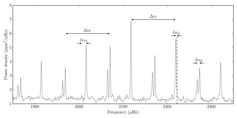
The frequency spectrum of a typical solar-type star observed by Kepler, Kepler-68 (KIC 11295426), is shown in Fig. 1. It depicts the power as a function of frequency with the radial order increasing with frequency, while the angular degree follows a regular pattern of alternating spherical degrees. The peaks with the largest amplitudes are located in the middle of the excited frequency range, and the centre of the power envelope defines the frequency of maximum oscillations power ().
The p-modes in a solar-like oscillator follow a regular structure. Dominating this regularity is the large frequency separation (), which is the average frequency spacing between modes with consecutive radial orders and the same angular degree. Observationally and theoretically is most commonly defined by the average separation of radial modes, since these frequencies are unaffected by frequency shifts due to mixed modes (since no radial g-modes exist).
The small frequency separations and are those between modes with a radial order that differs by unity and an angular degree that differs by two. These separations have also been indicated in Fig. 1 in addition to another small frequency separation, namely the offset of the peaks from the midway point between two modes with (). Deviations from regularity in the large and small frequency separations are due to rapid changes in the sound speed profile (so-called acoustic glitches), and hence are powerful diagnostics for infer the interior structure of stars.
Frequencies of high radial order and low angular degree can be described using asymptotic theory (Tassoul 1980). In this framework, the large frequency separation can be shown to be given by the inverse of the sound travel time across the stellar diameter (e.g. Aerts et al. 2010):
| (1) |
Here, is the sound speed and the stellar radius. The large frequency separation has been found to scale to a good approximation with the mean stellar density, while the small frequency separations are sensitive to the stellar age since they depend on the sound speed gradient in the deep stellar interior. This means that the frequency separations of a star of given mass and composition will vary in time as a result of stellar evolution.
3 Stellar properties from scaling relations
Scaling relations based on the average large frequency separation and the frequency of maximum oscillation power are a powerful way to determine fundamental stellar properties for a large number of stars. This approach can be used when the signal-to-noise ratio in the power spectrum is too low to allow for a reliable extraction of individual oscillation frequencies. In this section the scaling relations will be derived and discussed in terms of their accuracy and suggested modifications.
3.1 Scaling relations for and
Assuming adiabatic conditions and an ideal gas we can express the sound speed and temperature as and , where is the mean molecular weight. Substituting these expressions into Eq. 1, it can be seen that is proportional to the square root of the mean stellar density (Ulrich 1986; Kjeldsen and Bedding 1995; Bedding and Kjeldsen 2010):
| (2) |
with being the stellar mass. This implies that as a solar-type star expands during its evolution along the main sequence and beyond, the mean density and thus the large frequency separation will decrease.
The frequency of maximum power () is another observable that changes as a star evolves. This can be understood through its suggested scaling with the acoustic cut-off frequency (see for instance Brown et al. 1991; Kjeldsen and Bedding 1995; Belkacem et al. 2011). The acoustic cut-off frequency for an isothermal atmosphere is given by
| (3) |
being the density scale height, which is proportional to with being the surface gravity and the effective temperature. Thereby we have (Kjeldsen and Bedding 1995)
| (4) |
Thus, as above, when a solar-type star evolves, the frequency of maximum power decreases due to a decreasing surface gravity.
The scaling relations for and (Eqs. 2 and 4) can be combined with the stellar effective temperature to yield fundamental stellar properties such as mass and radius. It is worth noting, however, that these relations are extrapolated from the well known solar properties. Thus, an inherent assumption when using the scaling relations for stars ranging from the main sequence to red giant phases is that they are homologous to the Sun. In this manner, the following equations for mass, radius, surface gravity, and mean density are obtained:
| (5) |
| (6) |
| (7) |
| (8) |
This is sometimes referred to as the direct method to obtain fundamental properties, and it provides estimates that are independent of stellar evolutionary models under the assumption that the scaling relations are valid (see for instance Chaplin and Miglio 2013). It can be seen from Eqs. 5 and 6 that the determination of stellar mass is inherently more uncertain than that of the radius, since it depends more strongly on the parameters in the expression. The equations can also be written in several other ways, for instance using the relation between radius, temperature and luminosity; (see, for example, Bedding 2014).
A disadvantage of the direct method is that the propagated uncertainties for masses and radii can be significantly overestimated since our physical knowledge of stellar evolution is ignored (i.e., any combination of , and are allowed). Another disadvantage of the direct method is that it cannot estimate ages. These issues can be circumvented by instead adopting a grid-based modelling approach, where we compare the observed and to predictions from stellar evolutionary models. The ”best matching” models are then taken as having properties that closely match those of the target star. The approach for is straightforward: one applies a linear fit as a function of radial order to the theoretically computed frequencies of the stellar model weighted in a manner that mimics the analysis used to extract the observed from the real data (White et al. 2011). Unfortunately, matters are less straightforward for owing to shortcomings in non-adiabatic predictions of the excitation and damping of the modes (which are required to compute a model ). Instead, a common approach is to use the mass, radius and temperature of the model as input to the scaling relation to compute the model-predicted parameter.
3.2 Accuracy of the scaling relations
Equations 2 and 4 are approximate relations which require careful validation. Due to the wealth of space-based data and the complexity of modeling oscillation frequencies for large numbers of stars, many studies have relied on scaling relations and hence testing their accuracy has become one of the most active topics of research in asteroseismology.
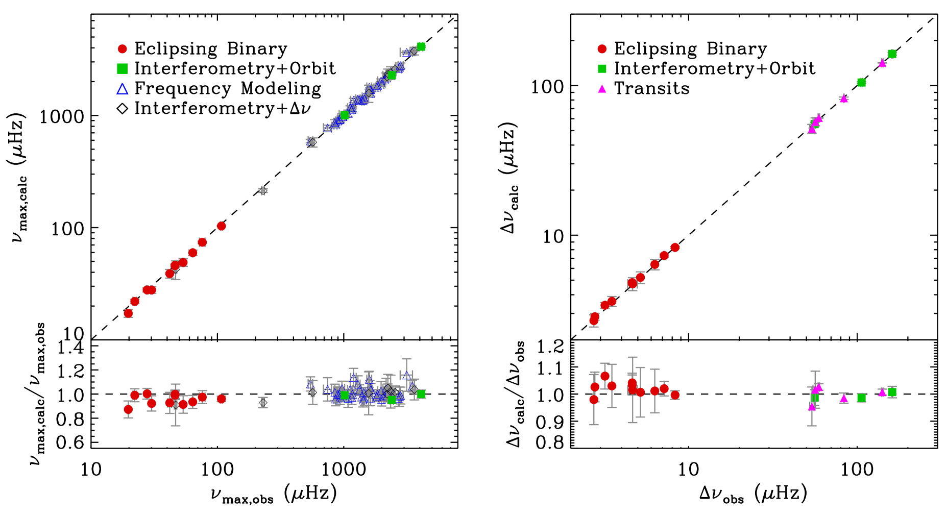
Density and Surface Gravity: Direct tests of Equations 2 and 4 require independent measurements of or density, which are typically only possible for eclipsing, spectroscopic binaries or the combination of interferometry with astrometric orbits. Figure 2 shows a comparison of measured and calculated and values for systems where such constraints are currently available. The comparison also includes densities derived from transiting exoplanets with independently constrained eccentricities such as HD17156 (Nutzman et al. 2011; Gilliland et al. 2011), TrES-2 (Southworth 2011; Barclay et al. 2012), HAT-P-7 (Christensen-Dalsgaard et al. 2010; Southworth 2011), Kepler-14 (Southworth 2012; Huber et al. 2013b), and Kepler-7 (Sandford and Kipping 2017). Furthermore, tests of through more indirect methods include combining interferometric angular diameters with densities calculated from the scaling relation, or masses and radii determined from individual frequency modeling (e.g., Metcalfe et al. 2014). Figure 2 demonstrates good agreement over three orders of magnitude, with median residuals indicating typical accuracies of 0.03 dex and 0.01 dex in for giants and dwarfs/subgiants, as well as 4% and 2% in density for giants and dwarfs/subgiants.
Stellar Masses: Figure 2 shows evidence that deviations increase for more evolved stars, as expected since scaling relations are anchored to the Sun. There has been mounting evidence that asteroseismic masses for red giants are overestimated by based on comparisons with dynamical masses from eclipsing binaries (Frandsen et al. 2013; Gaulme et al. 2016), cluster masses determined from near turn-off eclipsing binaries (Brogaard et al. 2012), and expectation values for luminous metal-poor () giants (Epstein et al. 2014). While the extent and dependence of this offset on evolutionary state is not yet clear, it indicates that masses for red giants from scaling relations should be broadly accurate to 10%. Independent masses of seismic dwarfs and subgiants are rare, but can be expected to better than 5%.
Stellar Radii: Tests of stellar radii typically result from the combination of angular diameters measured through optical long-baseline interferometry with parallaxes (Huber et al. 2012a; White et al. 2013; Johnson et al. 2014), followed by more indirect estimates from luminosities derived from parallaxes (Silva Aguirre et al. 2012; Huber et al. 2017) or clusters (Miglio 2012; Miglio et al. 2016). Figure 3 shows a summary of current empirical tests of radii from scaling relations. While no significant systematic offsets are evident for main-sequence stars (), comparisons to Gaia radii and eclipsing binaries show evidence for systematic differences at the 5% level for subgiants (1.5–3 ) and evolved red giants (8 ). Overall, these tests indicate that scaling relation radii are accurate to a few percent for dwarfs/subgiants and to within 5% for giants.
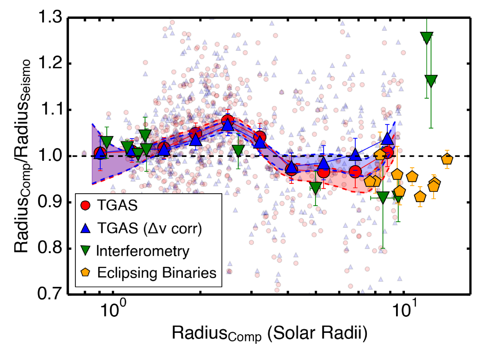
Scaling Relation Corrections: Due to the lack of empirical results spanning a large range of parameter space, corrections to scaling relations have so far mostly relied on theoretical work. Specifically, most proposed corrections have compared the average large frequency separation () calculated from individual frequencies with model densities (Stello et al. 2009; White et al. 2011; Guggenberger et al. 2016; Sharma et al. 2016) or suggested an extension of the asymptotic relation (Mosser et al. 2013). A consistent result is that scaling relation corrections should depend on , evolutionary state and metallicity, and first results have shown that such corrections indeed improve the agreement with independent constraints (Sharma et al. 2016; Huber et al. 2017). Uncertainties in modeling the driving and damping of oscillations typically prevent theoretical tests of the scaling relation, although some studies have shown encouraging results (Belkacem et al. 2011).
4 Stellar properties from individual frequencies
Instead of the global asteroseismic parameters, the individual oscillation frequencies can be used to infer stellar properties. The increase in the information content provided by the asteroseismic data leads to a higher precision than what can be achieved using and .
In this approach, the individual oscillation frequencies are compared to frequencies determined from stellar models in order to obtain the best possible agreement. In addition to the observed frequencies, the stellar effective temperature and metallicity are used as external observables to place extra constraints on the models. However, because of improper modelling of the near-surface layers, there is an offset between observed and computed oscillation frequencies, the so-called surface term or surface effect. Commonly, the offset is corrected using empirical or theoretically motivated schemes such as those proposed by Kjeldsen et al. (2008); Ball and Gizon (2014); Sonoi et al. (2015). It is possible to avoid the need for a correction if one fits frequency differences or frequency difference ratios instead, since these are combinations of frequencies that minimise the impact of the near-surface layers (e.g., Roxburgh and Vorontsov 2003; Silva Aguirre et al. 2011).
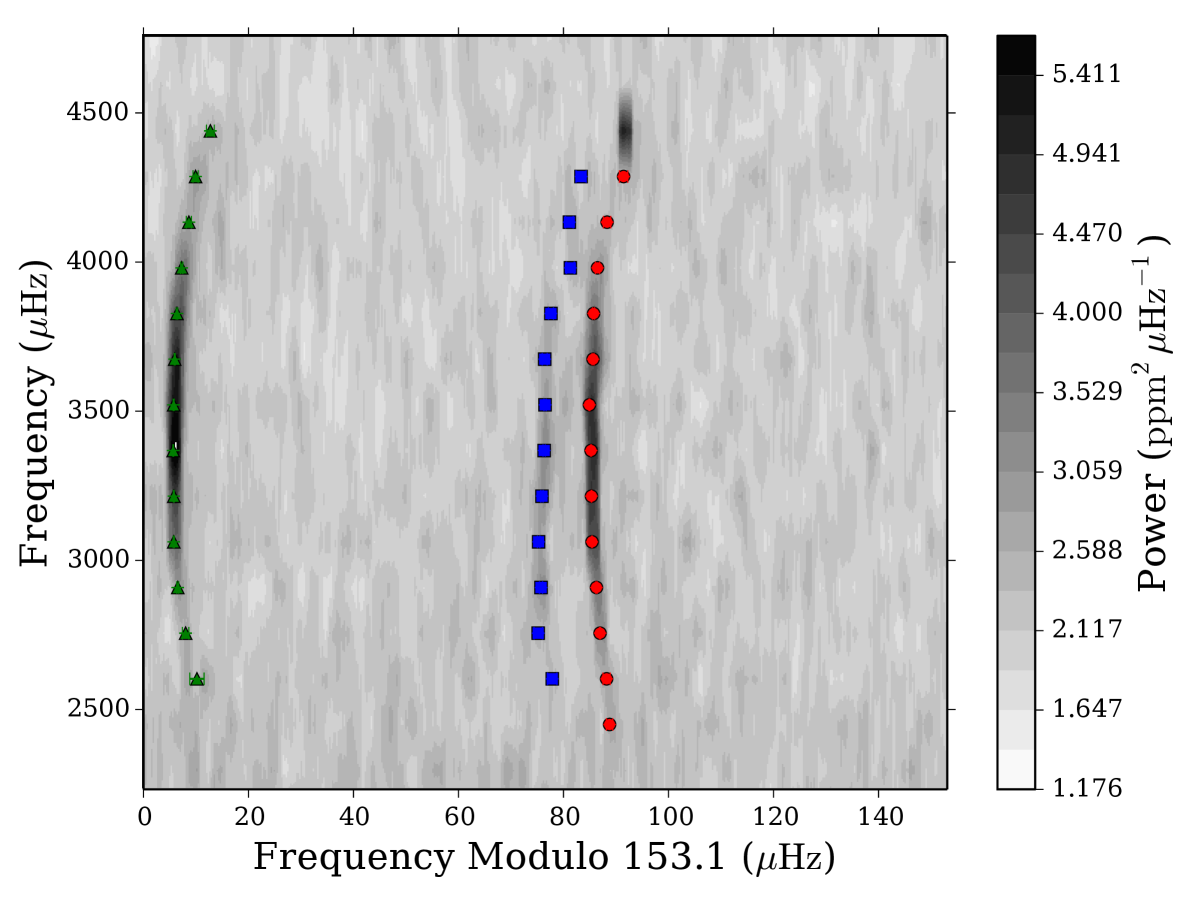
An example of a best-fitting model, i.e., a model that is able to reproduce the observed frequency spectrum, can be seen in Fig. 4. This échelle diagram (Grec et al. 1983) (or ladder diagram) is often used to display modelled and observed oscillation frequencies. It can be constructed by dividing the power spectrum into segments of length in frequency, and then stacking them on top of each other. The oscillation modes with the same angular degree will line up vertically, forming a separate ridge for each degree, with mixed modes showing a strong deviation from the ridge structure. If the frequency spacings did not vary with frequency, each ridge would be perfectly straight (and vertical if the correct is used), but since the spacings do change slightly with frequency, the ridges have some curvature.
In addition to constraining the fundamental stellar properties, including the age of the star, modelling the individual frequencies also allows determination of the surface helium abundance and the depth of the outer convection zone (e.g., Verma et al. 2014; Mazumdar et al. 2014). Not only can more parameters be constrained using detailed modelling of the observed frequencies, the precision on the fundamental properties is also improved compared to the global-parameters case. For of the best-quality solar-like stars observed by Kepler, Silva Aguirre et al. (2017) found average uncertainties of in radius, in mass and in age. Clearly both the radius and the age of the star can be determined to a high level of precision, which allows for precise planetary radii to be derived while having good knowledge of the age of the system.
5 Comparison of stellar properties from different methods
The level of precision achievable when determining stellar properties will not only depend on the uncertainties in the fitted observables, but also which observables that are being reproduced. Of particular importance for studies of planetary systems is the density of the host star, since an independent measurement of this parameter can be used in the transit fit to constrain the orbital eccentricity of an exoplanet (this is described in more detail later in this chapter). The stellar radius is also highly relevant as it, for a transiting planet, allows for the determination of the planetary radius (see Eq. 9). Figure 5 compares the obtained uncertainties in stellar density, radius and mass using asteroseismology, transits and spectroscopy for the sample of Kepler exoplanet hosts studied by Silva Aguirre et al. (2015).
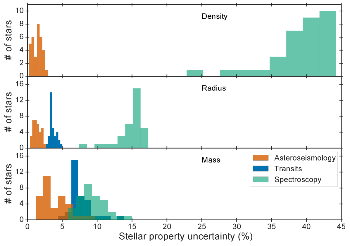
The spectroscopic uncertainties have been computed using measured uncertainties on the temperature and metallicity and assuming a constant uncertainty on of dex. In the case of the transit uncertainties, a constant uncertainty on the density of was assumed in addition to what was the case for the spectroscopic sample, since this is an optimistic estimate of the density uncertainty that can be determined from the transit. The asteroseismic uncertainties have been determined from fitting individual frequencies in addition to temperature and metallicity.
The figure illustrates that modelling individual frequencies tightly constrain the fractional uncertainties; for example all density uncertainties are below 3% and the median value is 1.7%, which is in stark contrast to the density uncertainties derived from spectroscopy where the uncertainty is larger than in all cases. More generally for all the parameters shown, asteroseismology provides the highest precision, followed by transits and then spectroscopy. For the stellar mass this is the least clear-cut, owing partly to the fact that - out of the three parameters shown - the mass is the least constrained directly from the asteroseismic information.
6 Asteroseismology of exoplanet hosts
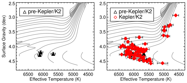
Especially since the launch of Kepler, asteroseismology has started to play an important role for the characterisation of exoplanets and exoplanet systems. This synergy has proven very powerful and has yielded many interesting results. To date, the sample of exoplanet host stars with an asteroseismic detection exceeds 100 with Kepler alone, if the host stars of planet candidates are also included (Huber et al. 2013b; Lundkvist et al. 2016). The sample before and after the launch of Kepler can be seen in Fig. 6, where it is evident that Kepler has spearheaded a transformation in the synergy between asteroseismology and exoplanet science.
The primary contribution of asteroseismology has been to determine highly precise host star radii, which translates into very precise planetary radii when combined with the transit depth (see Eq. 9). Some of the most precisely determined planetary radii have uncertainties as low as (Silva Aguirre et al. 2015), which in some cases correspond to km (see for instance Ballard et al. 2014; Fogtmann-Schulz et al. 2014).
Knowing the radius of a planet is important for understanding its composition, since composition models depend sensitively on this parameter. For instance, the transition from a rocky to a volatile-rich composition is estimated to take place at (Weiss and Marcy 2014; Rogers 2015). Uncertainties in the planetary radius can therefore cast doubt on whether a given exoplanet is rocky or gaseous. An example of this is the exoplanet Kepler-452b. It orbits a Sun-like star in the habitable zone, but has an uncertain radius just on the predicted threshold between rocky and gaseous (Jenkins et al. 2015). Therefore, it is very difficult to determine whether it is a rocky planet or not.
Why the stellar and planetary radii are so intimately linked can be understood by assuming that a planetary transit can be described as two spheres passing in front of each other. The transit depth () can then be found as (Seager and Mallén-Ornelas 2003)
| (9) |
with and being the planetary and stellar radius respectively. In practice, effects such as limb darkening and a non-zero impact parameter have to be taken into account. However, detailed modelling of the transit lightcurve can yield planet-to-star radius ratios that are precise enough that for of all planet candidates detected by Kepler the dominating contribution to the uncertainty on the planetary radius is the uncertainty on the stellar radius (Huber 2018). This is one of the reasons why asteroseismology is so important for the precise characterisation of exoplanets.
Another example is the Kepler-444 system. Here, using asteroseismology it has been possible to determine both precise radii and a precise age of the system, and to thereby establish that it is the oldest known system with terrestrial-sized exoplanets. The Kepler-444 system has an age of Gyr, which means that it formed when the Universe was about of its current age (Campante et al. 2015). The system is a compact system with five planets, which all have radii between those of Mercury and Venus and all orbit closer to their host star than Mercury does to the Sun. This results shows that small planets have formed throughout a large fraction of the history of the Universe. A pair of low-mass stellar companions in a highly eccentric orbit have also been detected in this system, which shows that the formation of small planets can also occur in a truncated protoplanetary disk (Dupuy et al. 2016).
6.1 Orbital eccentricities of small exoplanets
Knowing the eccentricity of an exoplanet’s orbit is important as it can hold clues to its formation and evolution and also impact its habitability. However, determining the eccentricity of small exoplanets is difficult with traditional methods, which favour large planets (Doppler velocities, Marcy et al. 2014) and a small subset of multiplanet systems (timing of secondary transits and transit timing variations, e.g. Hadden and Lithwick 2014). For an overview the reader is referred to Hadden and Lithwick (2017).
If an exoplanet is on an eccentric orbit, its orbital speed will change depending on its position in the orbit according to Kepler’s second law of motion. As a consequence, the observed transit duration will change depending on where in the orbit of the exoplanet the transit happens. If it occurs on a slow-moving part of the orbit, the transit duration will be longer than in the circular case, and vice versa if the transit takes place while the planet is on a fast moving portion of the orbit.
The transit duration for a transiting exoplanet moving on a circular orbit is governed by the mean stellar density (Seager and Mallén-Ornelas 2003). The mean stellar density assuming a circular orbit and the true stellar mean density are related as (e.g. Kipping 2010)
| (10) |
with being the eccentricity and the angle of periastron. Thereby, if the mean stellar density is known from another method, such as asteroseismology, transits can be used to constrain the orbital eccentricity of the exoplanet.
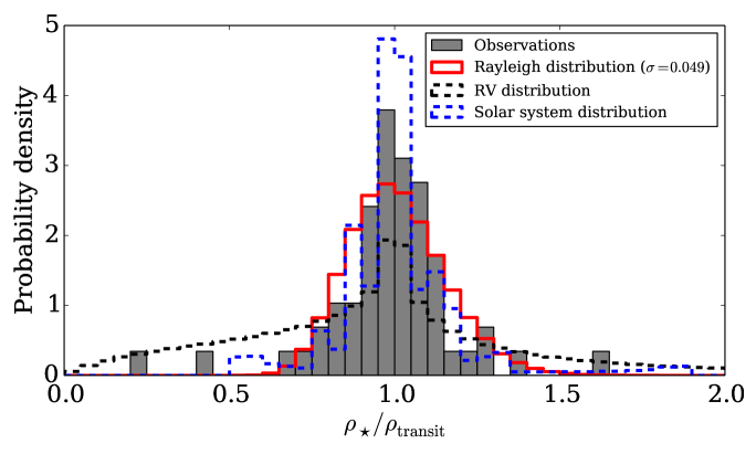
First studies combining asteroseismically determined stellar densities with those measured from transits for the Kepler sample were done by Sliski and Kipping (2014) and Van Eylen and Albrecht (2015). The latter investigated a sample of 28 multiplanet systems, which are expected to have a high fraction of true planets (Lissauer et al. 2012). A histogram of the derived ratio between seismic and transit density for their sample of 74 exoplanets can be seen in Fig. 7, which also includes a sample of planets with eccentricities determined from radial velocities and the solar system planets, for comparison. As is the case for the solar system, the sample with asteroseismology have ratios that are close to unity and thus consistent with circular orbits, something that is different to what is seen for the radial velocity sample that displays a wider range of ratios. Given that Kepler multiplanet systems preferentially contain small planets (Latham et al. 2011), this indicates that small planets tend to have circular orbits. This is an important result, not only because it may hold clues to understanding the evolution of these systems, but also because eccentricity can impact both the habitability of exoplanets and predicted occurrence rates (Van Eylen and Albrecht 2015).
The sample of planets with eccentricities was expanded by Xie et al. (2016) and Hadden and Lithwick (2017), although not using asteroseismology. Xie et al. (2016) used spectroscopically determined stellar densities to confirm that Kepler multiplanet systems indeed seem to have circular orbits, while single planet systems show larger eccentricities. That multiplanet systems have low eccentricities is in agreement with what was found by Hadden and Lithwick (2017) using transit timing variations, but they add that the eccentricity is in many cases non-zero. Further expanding these studies using asteroseismology to also investigate, for instance, single planet systems would be valuable to independently confirm the results by Xie et al. (2016) using a high precision sample.
6.2 Using precise planet properties to confirm evaporation
Super-Earths and sub-Neptunes are the most common type of planet found by Kepler (Borucki et al. 2011; Batalha et al. 2013; Marcy et al. 2014). In spite of this, a staggering absence of these planets in ultra short period orbits (USP planets) is evident in the Kepler data, which has been attributed to photo-evaporative stripping of the volatile-rich envelopes of these planets. That photo-evaporation plays a role in sculpting the population of hot, close-in planets has been predicted for some years (e.g. Lopez and Fortney 2013; Owen and Wu 2013), and the observational evidence to confirm this has been provided using asteroseismology. Lundkvist et al. (2016) performed an asteroseismic analysis of over 100 exoplanet host stars, harbouring in excess of 150 exoplanets, and used the very precise stellar radii and mean densities obtained to compute highly precise planet properties.
This was done by combining the stellar radius and mean density from asteroseismology with the orbital period of the planet and the ratio of planet to stellar radii (see Eq. 9). This allows for the planet radius to be found simply as the product of the stellar radius and the planet-to-star radius ratio. Including also the stellar effective temperature, the flux incident on the exoplanet from the star can be found from re-writing Kepler’s third law and combining it with the inverse-square law for the flux (Lundkvist et al. 2016):
| (11) |
Here, is the mean density, is the orbital period of the exoplanet, and is the effective temperature with the subscript indicating the star and the Sun.
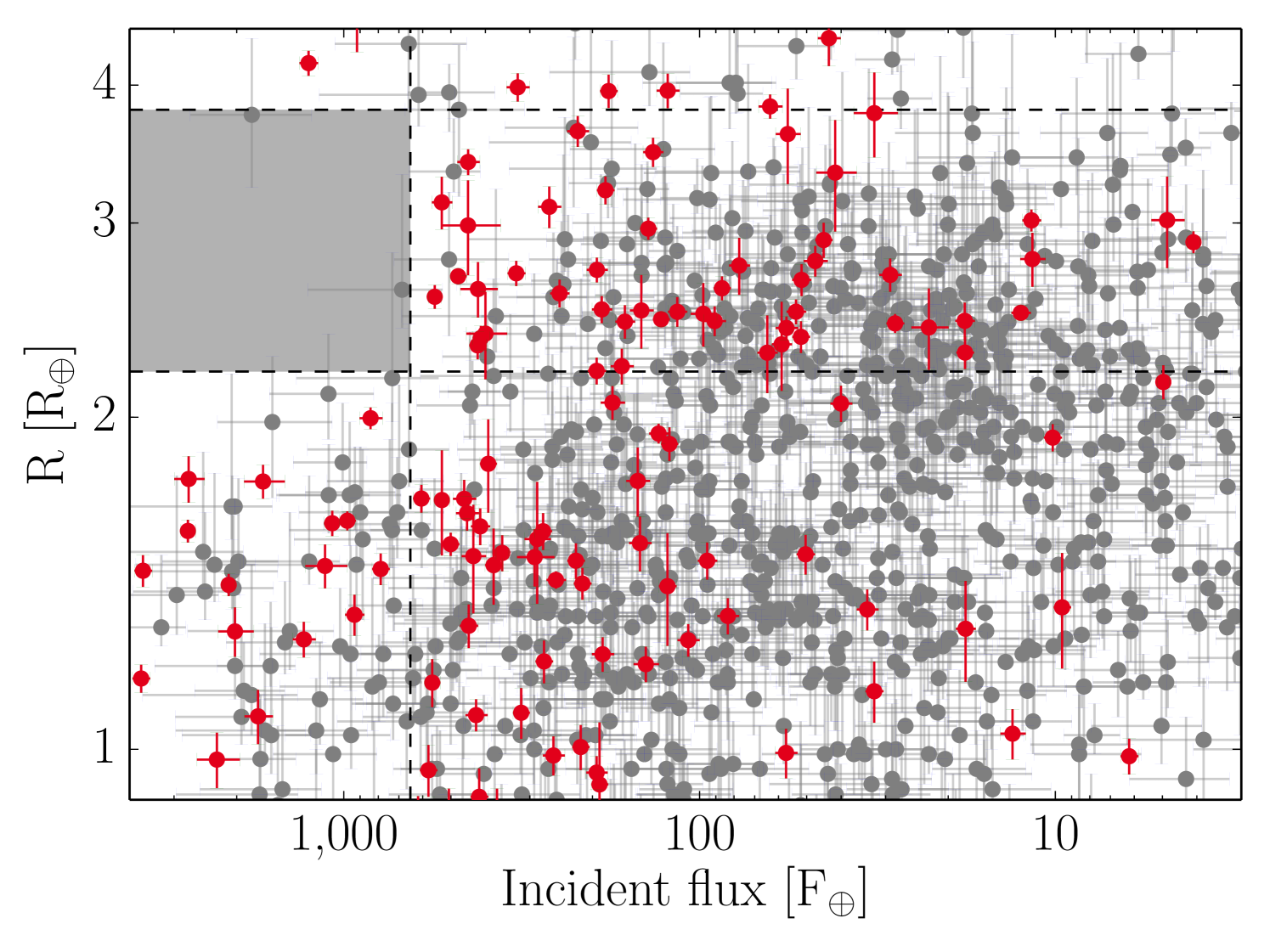
A desert of hot super-Earths/sub-Neptunes can be observed for USP planets when plotting the planetary radius against either the planetary period or the incident flux. This can be seen in the left panel of Fig. 8 for the incident flux. The shaded region highlights the evaporation desert found by Lundkvist et al. (2016); that is a region of parameter space void of exoplanets, which is consistent with the expected effect of photo-evaporation of volatile-rich atmospheres.
The observational confirmation of an evaporation desert emphasizes the importance of asteroseismology for obtaining precise exoplanetary properties, and additionally shows that evaporation plays an important role in shaping the exoplanet population that we see today. It can also be useful for constraining the formation of USP planets. For instance, it has been shown by Lopez (2017) that in order to recreate such an evaporation desert, the majority of USP planets must have formed from water-poor material.
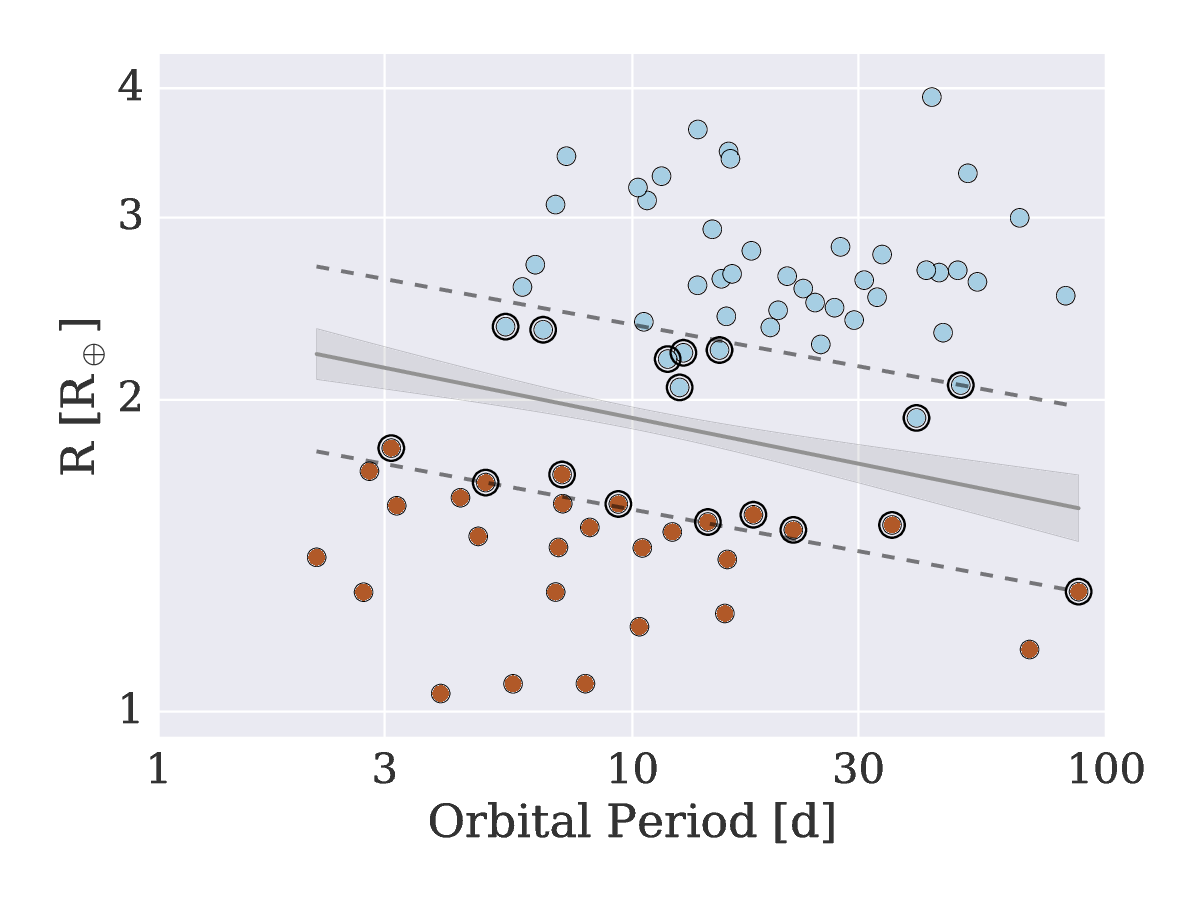
A recent breakthrough in our understanding of the radius distribution of small planets was achieved by Fulton et al. (2017), using a large sample of host stars with radii derived from high-resolution spectroscopy. Importantly the spectroscopic surface gravities and radii were calibrated against asteroseismology (Petigura et al. 2017), highlighting the importance of asteroseismology as a fundamental benchmark for more indirect methods. Fulton et al. (2017) investigated small, close-in planets with periods less than days and detected a bimodality in the size distribution with few planets having a radius between . They also found an evaporation valley consistent with predictions by Owen and Wu (2013) and Lopez and Fortney (2013). This deficit of planets with a radius along with clear evidence of an evaporation valley was also found by Van Eylen et al. (2017). They used the asteroseismic samples of exoplanet host stars by Silva Aguirre et al. (2015) and Lundkvist et al. (2016) along with new light curve modelling to derive very precise planetary radii and orbital periods.
A plot showing the planetary radius as a function of the period can be seen in the right panel of Fig. 8. Here, the evaporation valley and its slope are clearly visible, showing that the gap occurs at larger radii for lower orbital periods. Determining the slope of the valley is important, because, according to Lopez and Rice (2016) it speaks to the formation mechanism of the hot, short period super-Earths. They argue that a negative slope is consistent with that expected for photo-evaporation, while being inconsistent with exclusive late formation of gas-poor rocky planets. The slope of the evaporation valley thus indicates that a substantial fraction of short-period super-Earths originate from evaporation of planets with a significant envelope. According to Lopez and Rice (2016), this could impact the determination of the frequency of Earth-like planets in the habitable zone (), which further emphasizes the importance of understanding the formation of these hot, short-period super-Earths.
6.3 Spin-axis inclinations from rotational splittings
The obliquity or the spin-orbit angle () is the angle between the normal to the orbital plane of the exoplanet and the rotation axis of the host star. It is a valuable parameter to determine because of its importance for understanding the dynamical formation history and evolution of exoplanet systems.
The obliquity may be computed as (Fabrycky and Winn 2009)
| (12) |
Here, is the angle between the line of sight and the planetary orbital axis, is the inclination angle of the stellar rotation axis with respect to the line of sight, and is the angle between the sky projections of the stellar spin axis and the orbital plane of the exoplanet (the sky-projected spin-orbit angle). Figure 9 illustrates these angle in the HAT-P-7 system.
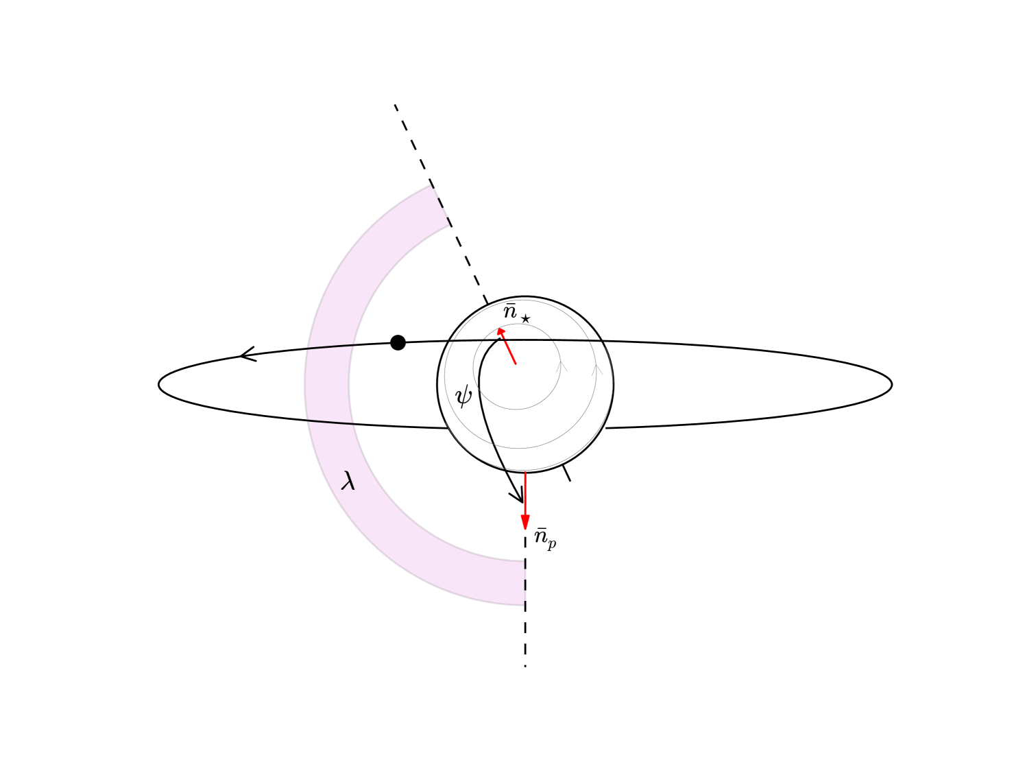
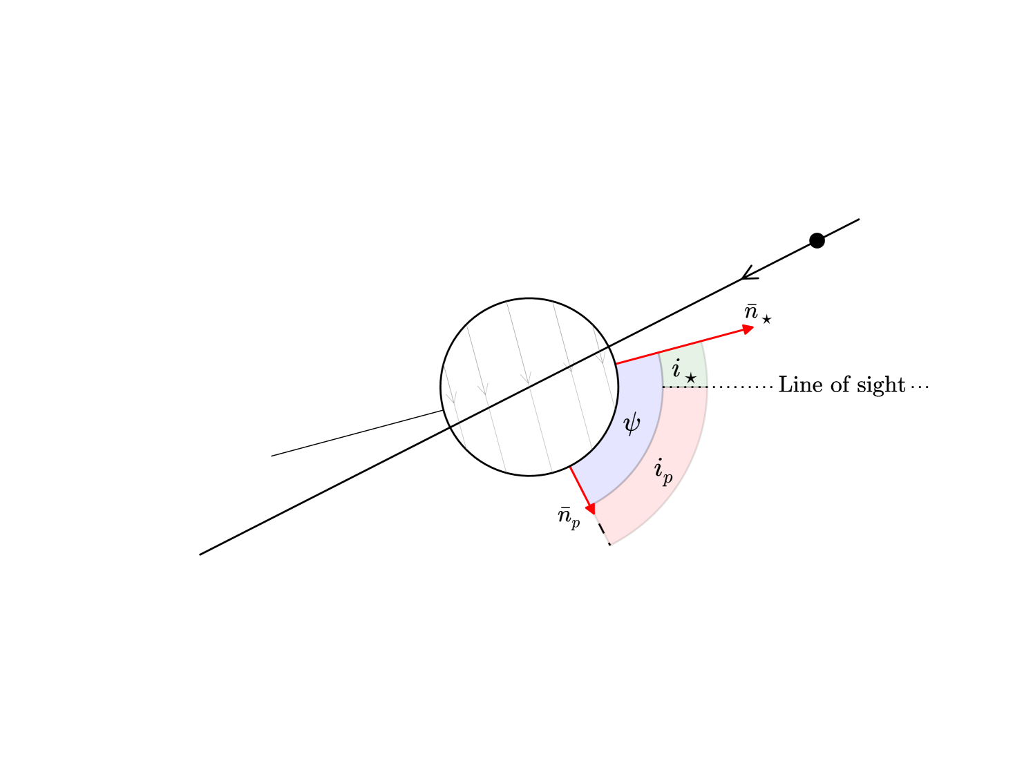
In the case of a transiting exoplanet, can normally be determined from the transit lightcurve (it will be ), and can be obtained through radial velocity observations during the transit (the Rossiter-McLaughlin effect). As alluded to earlier, the value of can be determined through asteroseismology by measuring relative amplitudes of rotationally split multiplets (Gizon and Solanki 2003). Thereby, using both information from the transit, from spectroscopic observations and from asteroseismology we can establish a full 3D view of the star-planet system.
One system for which this has been done is the HAT-P-7 system, shown schematically in Fig. 9 (Benomar et al. 2014; Lund et al. 2014). Here, it was found from the Rossiter-McLaughlin effect that the planet, HAT-P-7b, is likely orbiting against the stellar rotation (Winn et al. 2009; Narita et al. 2009; Albrecht et al. 2012), but without knowing the line of sight stellar inclination angle, the orbit of the planet could be retrograde or closer to polar. From asteroseismology it was determined that the star is viewed almost pole-on (, Lund et al. 2014), which indicates that the planet is most likely in a retrograde but near-polar orbit.
Often, it is not possible to determine the obliquity directly, since all the needed measurements are only available for a small number of systems. It is worth noting that for a transiting planet, if the stellar inclination angle is measured to be close to a pole-on view (), this indicates that the star-planet system is misaligned (high obliquity), since a transit shows that the orbital plane is (almost) aligned with the line of sight. However, a stellar inclination angle close to (equator-on view) does not necessarily imply an aligned system (see e.g. Campante et al. 2016).
Estimating the obliquity in a statistical fashion has been done for a number of systems using asteroseismology, including Kepler-50 and Kepler-65 (Chaplin et al. 2013), Kepler-410A (Van Eylen et al. 2014), Kepler-432 (Quinn et al. 2015) and 16 Cygni B (Davies et al. 2015). All multiplanet systems in these studies have been found to be well aligned, supporting the theory that high obliquities are confined to hot Jupiters and thus likely related to their formation (Winn et al. 2010; Albrecht et al. 2013, e.g.).
The first counterexample of this observed trend of well-aligned multiplanet systems was also provided by asteroseismology: Kepler-56, a red giant hosting two transiting planets (Huber et al. 2013a). Here, asteroseismology yielded an inclination angle of , which implies spin-orbit misalignment with an obliquity of (Li et al. 2014). Follow-up observations have confirmed a massive, non-transiting planet in a wide orbit in this system, which is believed to be responsible for the misalignment (Boué and Fabrycky 2014; Otor et al. 2016).
A study using an asteroseismic determination of the stellar inclination angle of 25 main sequence and sub-giant solar-like stars was carried out by Campante et al. (2016). They used the determined to place statistical constraints on the obliquity of the systems. They found that for the 25 systems in their sample, 6 of them are potentially misaligned (including HAT-P-7), but all systems are consistent with spin-orbit alignment within . Therefore, Kepler-56 is a unique example of an unambiguously misaligned multiplanet system. Further obliquity measurements using asteroseismology will be important in order to determine whether spin-orbit misalignments in multiplanet systems are common or not.
6.4 Other types of host stars
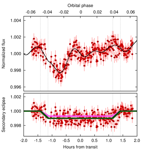
Asteroseismology of exoplanet hosts is not restricted to solar-like oscillators. One example of this is the host star WASP-33, which is orbited by the hot Jupiter WASP-33b and shows Scuti-type pulsations. These can be found in stars in the mass range from to (Pamyatnykh 2000; Murphy et al. 2017) and show larger pulsation amplitudes and fewer pulsation frequencies compared to the solar-like oscillators. von Essen et al. (2015) determined the temperature of the planet WASP-33b by measuring the depth of the secondary transit. However, as is also clear from Fig. 10, this was only possible after identifying the pulsation frequencies and removing them from the light curve, as the secondary eclipse was otherwise completely hidden within the signal from the stellar pulsations.
Another example could potentially come from the system with the hottest planet found to date; KELT-9 (or HD195689, Gaudi et al. 2017). The planet KELT-9b is hotter than some stars with a temperature exceeding K. The nominal temperature of the host star puts in between the classical instability strips for Scuti or slowly pulsating B stars, but future observations with improved precision may reveal pulsations since instability strip borders are not well-defined (Handler 2013). Additional high-impact studies could come from intermediate-mass host stars such as the Doradus pulsator HR8799 (Zerbi et al. 1999), for which space-based asteroseismology by missions such as TESS will dramatically improve our understanding of the age of the star and its directly imaged planets (e.g. Marois et al. 2010).
Mode identification in classical pulsators such as Scuti stars is challenging; however the extension of the asteroseismology-exoplanet synergy to these systems will without a doubt become more important in the near future. As an example, the photometric observations that will be provided over several years by the PLATO mission may give future opportunities to discover planets in wide orbits around Scuti stars by exploiting the small shifts in the pulsation frequencies induced by the planet. This method has already been used by Murphy et al. (2016) to detect a planet in an day orbit around its Scuti host star. At this orbital distance the planet is in or near the habitable zone, making it the first planet discovered within of the habitable zone around this type of star.
Acknowledgements.
The authors would like to thank Vincent Van Eylen, Carolina von Essen and Mikkel Lund for providing figures for this manuscript. Funding for the Stellar Astrophysics Centre is provided by The Danish National Research Foundation (Grant DNRF106). M.S.L. is supported by The Independent Research Fund Denmark’s Sapere Aude program (Grant agreement no.: DFF–5051-00130). D.H. acknowledges support by the National Aeronautics and Space Administration under Grant NNX14AB92G issued through the Kepler Participating Scientist Program. V.S.A. acknowledges support from the Villum Foundation (Research grant 10118). W.J.C. acknowledges support from the UK Science, Technology and Facilities Council (STFC).References
- Aerts et al. (2010) Aerts C, Christensen-Dalsgaard J Kurtz DW (2010) Asteroseismology. Springer
- Albrecht et al. (2012) Albrecht S, Winn JN, Johnson JA et al. (2012) Obliquities of Hot Jupiter Host Stars: Evidence for Tidal Interactions and Primordial Misalignments. ApJ757:18
- Albrecht et al. (2013) Albrecht S, Winn JN, Marcy GW et al. (2013) Low Stellar Obliquities in Compact Multiplanet Systems. ApJ771:11
- Ball and Gizon (2014) Ball WH Gizon L (2014) A new correction of stellar oscillation frequencies for near-surface effects. A&A568:A123
- Ballard et al. (2014) Ballard S, Chaplin WJ, Charbonneau D et al. (2014) Kepler-93b: A Terrestrial World Measured to within 120 km, and a Test Case for a New Spitzer Observing Mode. ApJ790:12
- Barclay et al. (2012) Barclay T, Huber D, Rowe JF et al. (2012) Photometrically Derived Masses and Radii of the Planet and Star in the TrES-2 System. ApJ761:53
- Batalha et al. (2013) Batalha NM, Rowe JF, Bryson ST et al. (2013) Planetary Candidates Observed by Kepler. III. Analysis of the First 16 Months of Data. ApJS204:24
- Bedding (2014) Bedding TR (2014) Solar-like oscillations: An observational perspective. In: Pallé PL Esteban C (eds) Asteroseismology, p 60
- Bedding and Kjeldsen (2010) Bedding TR Kjeldsen H (2010) Scaled oscillation frequencies and échelle diagrams as a tool for comparative asteroseismology. Communications in Asteroseismology 161:3–15
- Bedding et al. (2004) Bedding TR, Kjeldsen H, Butler RP et al. (2004) Oscillation Frequencies and Mode Lifetimes in Centauri A. ApJ614:380–385
- Belkacem et al. (2011) Belkacem K, Goupil MJ, Dupret MA et al. (2011) The underlying physical meaning of the max - c relation. A&A530:A142
- Benomar et al. (2014) Benomar O, Masuda K, Shibahashi H Suto Y (2014) Determination of three-dimensional spin-orbit angle with joint analysis of asteroseismology, transit lightcurve, and the Rossiter-McLaughlin effect: Cases of HAT-P-7 and Kepler-25. PASJ66:94
- Borucki et al. (2011) Borucki WJ, Koch DG, Basri G et al. (2011) Characteristics of Planetary Candidates Observed by Kepler. II. Analysis of the First Four Months of Data. ApJ736:19
- Bouchy and Carrier (2001) Bouchy F Carrier F (2001) P-mode observations on Cen A. A&A374:L5–L8
- Boué and Fabrycky (2014) Boué G Fabrycky DC (2014) Compact Planetary Systems Perturbed by an Inclined Companion. II. Stellar Spin-Orbit Evolution. ApJ789:111
- Brogaard et al. (2012) Brogaard K, VandenBerg DA, Bruntt H et al. (2012) Age and helium content of the open cluster NGC 6791 from multiple eclipsing binary members. II. Age dependencies and new insights. A&A543:A106
- Brown et al. (1991) Brown TM, Gilliland RL, Noyes RW Ramsey LW (1991) Detection of possible p-mode oscillations on Procyon. ApJ368:599–609
- Campante et al. (2015) Campante TL, Barclay T, Swift JJ et al. (2015) An Ancient Extrasolar System with Five Sub-Earth-size Planets. ApJ799:170
- Campante et al. (2016) Campante TL, Lund MN, Kuszlewicz JS et al. (2016) Spin-Orbit Alignment of Exoplanet Systems: Ensemble Analysis Using Asteroseismology. ApJ819:85
- Chaplin and Miglio (2013) Chaplin WJ Miglio A (2013) Asteroseismology of Solar-Type and Red-Giant Stars. ARA&A51:353–392
- Chaplin et al. (2013) Chaplin WJ, Sanchis-Ojeda R, Campante TL et al. (2013) Asteroseismic Determination of Obliquities of the Exoplanet Systems Kepler-50 and Kepler-65. ApJ766:101
- Chaplin et al. (2014) Chaplin WJ, Basu S, Huber D et al. (2014) Asteroseismic Fundamental Properties of Solar-type Stars Observed by the NASA Kepler Mission. ApJS210:1
- Christensen-Dalsgaard et al. (2010) Christensen-Dalsgaard J, Kjeldsen H, Brown TM et al. (2010) Asteroseismic Investigation of Known Planet Hosts in the Kepler Field. ApJ713:L164–L168
- Davies et al. (2015) Davies GR, Chaplin WJ, Farr WM et al. (2015) Asteroseismic inference on rotation, gyrochronology and planetary system dynamics of 16 Cygni. MNRAS446:2959–2966
- Dupuy et al. (2016) Dupuy TJ, Kratter KM, Kraus AL et al. (2016) Orbital Architectures of Planet-hosting Binaries. I. Forming Five Small Planets in the Truncated Disk of Kepler-444A. ApJ817:80
- Epstein et al. (2014) Epstein CR, Elsworth YP, Johnson JA et al. (2014) Testing the Asteroseismic Mass Scale Using Metal-poor Stars Characterized with APOGEE and Kepler. ApJ785:L28
- Fabrycky and Winn (2009) Fabrycky DC Winn JN (2009) Exoplanetary Spin-Orbit Alignment: Results from the Ensemble of Rossiter-McLaughlin Observations. ApJ696:1230–1240
- Fogtmann-Schulz et al. (2014) Fogtmann-Schulz A, Hinrup B, Van Eylen V et al. (2014) Accurate Parameters of the Oldest Known Rocky-exoplanet Hosting System: Kepler-10 Revisited. ApJ781:67
- Frandsen et al. (2013) Frandsen S, Lehmann H, Hekker S et al. (2013) KIC 8410637: a 408-day period eclipsing binary containing a pulsating giant star. A&A556:A138
- Fulton et al. (2017) Fulton BJ, Petigura EA, Howard AW et al. (2017) The California-Kepler Survey. III. A Gap in the Radius Distribution of Small Planets. AJ154:109
- Gaudi et al. (2017) Gaudi BS, Stassun KG, Collins KA et al. (2017) A giant planet undergoing extreme-ultraviolet irradiation by its hot massive-star host. Nature546:514–518
- Gaulme et al. (2016) Gaulme P, McKeever J, Jackiewicz J et al. (2016) Testing the Asteroseismic Scaling Relations for Red Giants with Eclipsing Binaries Observed by Kepler. ApJ832:121
- Gilliland et al. (2011) Gilliland RL, McCullough PR, Nelan EP et al. (2011) Asteroseismology of the Transiting Exoplanet Host HD 17156 with Hubble Space Telescope Fine Guidance Sensor. ApJ726:17
- Gizon and Solanki (2003) Gizon L Solanki SK (2003) Determining the Inclination of the Rotation Axis of a Sun-like Star. ApJ589:1009–1019
- Grec et al. (1983) Grec G, Fossat E Pomerantz MA (1983) Full-disk observations of solar oscillations from the geographic South Pole - Latest results. Sol Phys82:55–66
- Guggenberger et al. (2016) Guggenberger E, Hekker S, Basu S Bellinger E (2016) Significantly improving stellar mass and radius estimates: a new reference function for the scaling relation. MNRAS460:4277–4281
- Hadden and Lithwick (2014) Hadden S Lithwick Y (2014) Densities and Eccentricities of 139 Kepler Planets from Transit Time Variations. ApJ787:80
- Hadden and Lithwick (2017) Hadden S Lithwick Y (2017) Kepler Planet Masses and Eccentricities from TTV Analysis. AJ154:5
- Handler (2013) Handler G (2013) Asteroseismology. In: Oswalt TD Barstow MA (eds) Planets, Stars and Stellar Systems. Volume 4: Stellar Structure and Evolution, Springer, p 207
- Huber (2015) Huber D (2015) Asteroseismology of Eclipsing Binary Stars. In: Giants of Eclipse: The zeta Aurigae Stars and Other Binary Systems, Astrophysics and Space Science Library, vol 408, p 169, DOI 10.1007/978-3-319-09198-3˙7
- Huber (2018) Huber D (2018) Synergies Between Asteroseismology and Exoplanetary Science. Asteroseismology and Exoplanets: Listening to the Stars and Searching for New Worlds 49:119
- Huber et al. (2012a) Huber D, Ireland MJ, Bedding TR et al. (2012a) Fundamental Properties of Stars Using Asteroseismology from Kepler and CoRoT and Interferometry from the CHARA Array. ApJ760:32
- Huber et al. (2012b) Huber D, Ireland MJ, Bedding TR et al. (2012b) Validation of the exoplanet Kepler-21b using PAVO/CHARA long-baseline interferometry. MNRAS423:L16–L20
- Huber et al. (2013a) Huber D, Carter JA, Barbieri M et al. (2013a) Stellar Spin-Orbit Misalignment in a Multiplanet System. Science 342:331–334
- Huber et al. (2013b) Huber D, Chaplin WJ, Christensen-Dalsgaard J et al. (2013b) Fundamental Properties of Kepler Planet-candidate Host Stars using Asteroseismology. ApJ767:127
- Huber et al. (2017) Huber D, Bryson ST, Haas MR et al. (2017) The K2 Ecliptic Plane Input Catalog (EPIC) and Stellar Classifications of 138,600 Targets in Campaigns 1-8. ApJ224:2
- Jenkins et al. (2015) Jenkins JM, Twicken JD, Batalha NM et al. (2015) Discovery and Validation of Kepler-452b: A 1.6 R⨁ Super Earth Exoplanet in the Habitable Zone of a G2 Star. AJ150:56
- Johnson et al. (2014) Johnson JA, Huber D, Boyajian T et al. (2014) The Physical Parameters of the Retired a Star HD 185351. ApJ794:15
- Kipping (2010) Kipping DM (2010) Investigations of approximate expressions for the transit duration. MNRAS407:301–313
- Kjeldsen and Bedding (1995) Kjeldsen H Bedding TR (1995) Amplitudes of stellar oscillations: the implications for asteroseismology. A&A293:87–106
- Kjeldsen et al. (2008) Kjeldsen H, Bedding TR Christensen-Dalsgaard J (2008) Correcting Stellar Oscillation Frequencies for Near-Surface Effects. ApJ683:L175
- Latham et al. (2011) Latham DW, Rowe JF, Quinn SN et al. (2011) A First Comparison of Kepler Planet Candidates in Single and Multiple Systems. ApJ732:L24
- Li et al. (2014) Li G, Naoz S, Valsecchi F, Johnson JA Rasio FA (2014) The Dynamics of the Multi-planet System Orbiting Kepler-56. ApJ794:131
- Lissauer et al. (2012) Lissauer JJ, Marcy GW, Rowe JF et al. (2012) Almost All of Kepler’s Multiple-planet Candidates Are Planets. ApJ750:112
- Lopez (2017) Lopez ED (2017) Born dry in the photoevaporation desert: Kepler’s ultra-short-period planets formed water-poor. MNRAS472:245–253
- Lopez and Fortney (2013) Lopez ED Fortney JJ (2013) The Role of Core Mass in Controlling Evaporation: The Kepler Radius Distribution and the Kepler-36 Density Dichotomy. ApJ776:2
- Lopez and Rice (2016) Lopez ED Rice K (2016) Predictions for the Period Dependence of the Transition Between Rocky Super-Earths and Gaseous Sub-Neptunes and Implications for . ArXiv e-prints: 1610.09390
- Lund et al. (2014) Lund MN, Lundkvist M, Silva Aguirre V et al. (2014) Asteroseismic inference on the spin-orbit misalignment and stellar parameters of HAT-P-7. A&A570:A54
- Lundkvist et al. (2016) Lundkvist MS, Kjeldsen H, Albrecht S et al. (2016) Hot super-Earths stripped by their host stars. Nature Communications 7:11201
- Marcy et al. (2014) Marcy GW, Isaacson H, Howard AW et al. (2014) Masses, Radii, and Orbits of Small Kepler Planets: The Transition from Gaseous to Rocky Planets. ApJS210:20
- Marois et al. (2010) Marois C, Zuckerman B, Konopacky QM, Macintosh B Barman T (2010) Images of a fourth planet orbiting HR 8799. Nature468:1080–1083
- Mazumdar et al. (2014) Mazumdar A, Monteiro MJPFG, Ballot J et al. (2014) MEASUREMENT OF ACOUSTIC GLITCHES IN SOLAR-TYPE STARS FROM OSCILLATION FREQUENCIES OBSERVED BY KEPLER. ApJ 782(1):18
- Metcalfe et al. (2014) Metcalfe TS, Creevey OL, Doğan G et al. (2014) Properties of 42 Solar-type Kepler Targets from the Asteroseismic Modeling Portal. ApJS214:27
- Miglio (2012) Miglio A (2012) Asteroseismology of red giants as a tool for studying stellar populations: first steps. In: Miglio A, Montalbán J Noels A (eds) Red Giants as Probes of the Structure and Evolution of the Milky Way, Berlin: Springer, ApSS Proceedings
- Miglio et al. (2016) Miglio A, Chaplin WJ, Brogaard K et al. (2016) Detection of solar-like oscillations in relics of the Milky Way: asteroseismology of K giants in M4 using data from the NASA K2 mission. MNRAS461:760–765
- Mosser et al. (2013) Mosser B, Michel E, Belkacem K et al. (2013) Asymptotic and measured large frequency separations. A&A550:A126
- Murphy et al. (2016) Murphy SJ, Bedding TR Shibahashi H (2016) A Planet in an 840 Day Orbit around a Kepler Main-sequence A Star Found from Phase Modulation of Its Pulsations. ApJ827:L17
- Murphy et al. (2017) Murphy SJ, Moe M, Kurtz DW et al. (2017) Finding binaries from phase modulation of pulsating stars with Kepler: V. Orbital parameters, with eccentricity and mass-ratio distributions of 341 new binaries. ArXiv e-prints: 1712.00022
- Narita et al. (2009) Narita N, Sato B, Hirano T Tamura M (2009) First Evidence of a Retrograde Orbit of a Transiting Exoplanet HAT-P-7b. PASJ61:L35–L40
- Nutzman et al. (2011) Nutzman P, Gilliland RL, McCullough PR et al. (2011) Precise Estimates of the Physical Parameters for the Exoplanet System HD 17156 Enabled by Hubble Space Telescope Fine Guidance Sensor Transit and Asteroseismic Observations. ApJ726:3
- Otor et al. (2016) Otor OJ, Montet BT, Johnson JA et al. (2016) The Orbit and Mass of the Third Planet in the Kepler-56 System. AJ152:165
- Owen and Wu (2013) Owen JE Wu Y (2013) Kepler Planets: A Tale of Evaporation. ApJ775:105
- Pamyatnykh (2000) Pamyatnykh AA (2000) Pulsational Instability Domain of Scuti Variables. In: Breger M Montgomery M (eds) Delta Scuti and Related Stars, Astronomical Society of the Pacific Conference Series, vol 210, p 215
- Petigura et al. (2017) Petigura EA, Howard AW, Marcy GW et al. (2017) The California-Kepler Survey. I. High-resolution Spectroscopy of 1305 Stars Hosting Kepler Transiting Planets. AJ154:107
- Pietrinferni et al. (2004) Pietrinferni A, Cassisi S, Salaris M Castelli F (2004) A Large Stellar Evolution Database for Population Synthesis Studies. I. Scaled Solar Models and Isochrones. ApJ612:168–190
- Quinn et al. (2015) Quinn SN, White TR, Latham DW et al. (2015) Kepler-432: A Red Giant Interacting with One of its Two Long-period Giant Planets. ApJ803:49
- Rogers (2015) Rogers LA (2015) Most 1.6 Earth-radius Planets are Not Rocky. ApJ801:41
- Roxburgh and Vorontsov (2003) Roxburgh IW Vorontsov SV (2003) The ratio of small to large separations of acoustic oscillations as a diagnostic of the interior of solar-like stars. A&A411:215–220
- Sandford and Kipping (2017) Sandford E Kipping D (2017) Know the Planet, Know the Star: Precise Stellar Densities from Kepler Transit Light Curves. AJ154:228
- Seager and Mallén-Ornelas (2003) Seager S Mallén-Ornelas G (2003) A Unique Solution of Planet and Star Parameters from an Extrasolar Planet Transit Light Curve. ApJ585:1038–1055
- Sharma et al. (2016) Sharma S, Stello D, Bland-Hawthorn J, Huber D Bedding TR (2016) Stellar Population Synthesis Based Modeling of the Milky Way Using Asteroseismology of 13,000 Kepler Red Giants. ApJ822:15
- Silva Aguirre et al. (2011) Silva Aguirre V, Ballot J, Serenelli AM Weiss A (2011) Constraining mixing processes in stellar cores using asteroseismology. Impact of semiconvection in low-mass stars. A&A 529:63
- Silva Aguirre et al. (2012) Silva Aguirre V, Casagrande L, Basu S et al. (2012) Verifying Asteroseismically Determined Parameters of Kepler Stars Using Hipparcos Parallaxes: Self-consistent Stellar Properties and Distances. ApJ757:99
- Silva Aguirre et al. (2015) Silva Aguirre V, Davies GR, Basu S et al. (2015) Ages and fundamental properties of Kepler exoplanet host stars from asteroseismology. MNRAS452:2127–2148
- Silva Aguirre et al. (2017) Silva Aguirre V, Lund MN, Antia HM et al. (2017) Standing on the Shoulders of Dwarfs: the Kepler Asteroseismic LEGACY Sample. II.Radii, Masses, and Ages. ApJ835:173
- Sliski and Kipping (2014) Sliski DH Kipping DM (2014) A High False Positive Rate for Kepler Planetary Candidates of Giant Stars using Asterodensity Profiling. ApJ788:148
- Sonoi et al. (2015) Sonoi T, Samadi R, Belkacem K et al. (2015) Surface-effect corrections for solar-like oscillations using 3D hydrodynamical simulations. I. Adiabatic oscillations. A&A583:A112
- Southworth (2011) Southworth J (2011) Homogeneous studies of transiting extrasolar planets - IV. Thirty systems with space-based light curves. MNRAS417:2166–2196
- Southworth (2012) Southworth J (2012) Homogeneous studies of transiting extrasolar planets - V. New results for 38 planets. MNRAS426:1291–1323
- Stello et al. (2009) Stello D, Chaplin WJ, Basu S, Elsworth Y Bedding TR (2009) The relation between and max for solar-like oscillations. MNRAS400:L80–L84
- Tassoul (1980) Tassoul M (1980) Asymptotic approximations for stellar nonradial pulsations. ApJS43:469–490
- Ulrich (1986) Ulrich RK (1986) Determination of stellar ages from asteroseismology. ApJ306:L37–L40
- Van Eylen and Albrecht (2015) Van Eylen V Albrecht S (2015) Eccentricity from Transit Photometry: Small Planets in Kepler Multi-planet Systems Have Low Eccentricities. ApJ808:126
- Van Eylen et al. (2014) Van Eylen V, Lund MN, Silva Aguirre V et al. (2014) What Asteroseismology can do for Exoplanets: Kepler-410A b is a Small Neptune around a Bright Star, in an Eccentric Orbit Consistent with Low Obliquity. ApJ782:14
- Van Eylen et al. (2017) Van Eylen V, Agentoft C, Lundkvist MS et al. (2017) An asteroseismic view of the radius valley: stripped cores, not born rocky. ArXiv e-prints: 1710.05398
- Verma et al. (2014) Verma K, Faria JP, Antia HM et al. (2014) ASTEROSEISMIC ESTIMATE OF HELIUM ABUNDANCE OF A SOLAR ANALOG BINARY SYSTEM. The Astrophysical Journal 790(2):138
- von Essen et al. (2015) von Essen C, Mallonn M, Albrecht S et al. (2015) A temperature inversion in WASP-33b? Large Binocular Telescope occultation data confirm significant thermal flux at short wavelengths. A&A584:A75
- Weiss and Marcy (2014) Weiss LM Marcy GW (2014) The Mass-Radius Relation for 65 Exoplanets Smaller than 4 Earth Radii. ApJ783:L6
- White et al. (2011) White TR, Bedding TR, Stello D et al. (2011) Calculating Asteroseismic Diagrams for Solar-like Oscillations. ApJ743:161
- White et al. (2013) White TR, Huber D, Maestro V et al. (2013) Interferometric radii of bright Kepler stars with the CHARA Array: theta Cygni and 16 Cygni A and B. MNRAS433:1262–1270
- Winn et al. (2009) Winn JN, Johnson JA, Albrecht S et al. (2009) HAT-P-7: A Retrograde or Polar Orbit, and a Third Body. ApJ703:L99–L103
- Winn et al. (2010) Winn JN, Fabrycky D, Albrecht S Johnson JA (2010) Hot Stars with Hot Jupiters Have High Obliquities. ApJ718:L145–L149
- Xie et al. (2016) Xie JW, Dong S, Zhu Z et al. (2016) Exoplanet orbital eccentricities derived from LAMOST-Kepler analysis. Proceedings of the National Academy of Science 113:11,431–11,435
- Zerbi et al. (1999) Zerbi FM, Rodríguez E, Garrido R et al. (1999) The gamma DOR variable HR 8799: results from a multisite campaign. MNRAS303:275–283