Using Loaded N-port Structures
to Achieve the Continuous-Space
Electromagnetic Channel Capacity Bound
Abstract
A method for achieving the continuous-space electromagnetic channel capacity bound using loaded -port structures is described. It is relevant for the design of compact multiple-input multiple-output (MIMO) antennas that can achieve channel capacity bounds when constrained by size. The method is not restricted to a specific antenna configuration and a closed-form expression for the channel capacity limits are provided with various constraints. Furthermore, using loaded -port structures to represent arbitrary antenna geometries, an efficient optimization approach is proposed for finding the optimum MIMO antenna design that achieves the channel capacity bounds. Simulation results of the channel capacity bounds achieved using our MIMO antenna design with one square wavelength size are provided. These show that at least 18 ports can be supported in one square wavelength and achieve the continuous-space electromagnetic channel capacity bound. The results demonstrate that our method can link continuous-space electromagnetic channel capacity bounds to MIMO antenna design.
Index Terms:
Beamspace, channel capacity, continuous space, electromagnetic field, information theoryI Introduction
Information theory has been widely applied to the analysis and design of wireless communication systems to approach theoretical capacity limits [1]-[3]. However, the physical realization of wireless communication systems is based on the implementation of antennas and radio-frequency (RF) circuits [4], [5]. Therefore, the joint study of information theory and electromagnetic field theory can be utilized to further extend the theoretical channel capacity limits of the entire wireless communication system. This has led to the development of electromagnetic information theory (EIT) [6], [7]. Utilizing EIT, the concept of aerial degrees-of-freedom (ADoF) has been introduced to estimate the number of orthogonal basis functions required for describing electromagnetic fields around antenna systems [8]. The number of ADoF can be used to determine the channel capacity because it refers to the maximum number of parallel sub-channels that can be used for transmission [9]. To estimate the channel capacity bound for excitations restricted to a given volume or area, continuous current sources limited to a region, exciting the electromagnetic channel, have been analyzed using continuous-space approaches [10]-[12]. The results can be used to provide achievable bounds on the channel capacity given a specific volume or area. However, they have not provided the corresponding antenna designs to achieve those bounds.
Multiple-input multiple-output (MIMO) antenna systems, which exploit ADoF by using multiple antennas at transceivers, play a critical role in approaching the predicted channel capacity bounds in wireless communication systems [13]. As a result, an enormous number of MIMO antenna designs have been proposed [14]-[16]. A particular emphasis of these designs has been to devise approaches that achieve as many antennas as possible within a certain volume or area [17] and one example has provided up to 22 antennas per square wavelength [18]. These designs have to tradeoff strong mutual coupling effects with performance and this has led to design limits on the antennas possible per unit volume or area [19]. As a result, the analysis of the effects of mutual coupling on channel capacity performance have also been well studied [20], [21]. However there has been no direct link that can connect the design of MIMO antennas with the continuous-space approaches utilized in EIT [7], [22].
In this paper we introduce a method to link the antenna geometry and continuous-space electromagnetic channel capacity together by using loaded -port structures [23]-[25]. It is an attempt to bridge the gap between the practical design of MIMO antennas and their design limits predicted by EIT. This method is not restricted to a specific antenna configuration and uses the beamspace representation of MIMO systems. In beamspace MIMO, orthogonal radiation patterns also form independent sub-channels in a similar manner to the spatial separation of antennas that form spatial sub-channels [26]. Therefore, field distributions in the far-field can be linked with the capacity analysis in beamspace MIMO [27], [28] where the closed-form expression for the channel capacity limits [29], [30] are provided with various constraints. Furthermore, by using loaded -port structures to represent arbitrary antenna geometries, an efficient optimization approach is proposed for finding the optimum MIMO antenna design that achieves the channel capacity bounds. Simulation results of the channel capacity bounds and achieved capacity using our proposed antenna design with one wavelength square size are provided. These show the designed antenna can achieve capacity performance close to the fundamental bounds, demonstrating the effectiveness of the proposed method.
Organization: Section II formulates the MIMO system model for the loaded -port structures. Section III provides the derivation for the resultant channel capacity with different constraints. Section IV introduces the link with antenna design and describes efficient optimization approaches to obtain the optimum antenna configuration. In Section V, we provide numerical results of channel capacity for a proposed MIMO antenna design to demonstrate the potential of the technique. Section VI concludes the work.
Notation: Bold lower and upper case letters denote vectors and matrices respectively. Upper case letters in calligraphy denote sets. Letters not in bold font represent scalars. denotes the expectation of scalar . and refer to the th entry and norm of vector , respectively. , , , and refer to the transpose, conjugate transpose, th entry, determinant, and trace of a matrix , respectively. denotes complex number sets and denotes an imaginary number. denotes complex Gaussian distribution with mean and variance . denotes an identity matrix. diag is a diagonal matrix with diagonal entries being . refers to the inner product of two vectors and . It should also be noted that the dependence of all variables on frequency is assumed and it is not explicitly shown for brevity.
II System Model
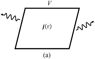
In Fig. 1(a) an arbitrary transmit element is shown, confined to a volume , with current distribution , where is the spatial coordinate. When matched with the proper receive element and channel, and with the current distribution appropriately set, the resulting system can achieve the continuous-space electromagnetic channel capacity bound [11]. Our objective in this work is to design the optimum MIMO antenna that can best approximate the required current distribution in to approach the continuous-space electromagnetic channel capacity bound. The challenge is to find structures that can create the necessary current distribution with the discrete feeding ports required in MIMO antenna design.
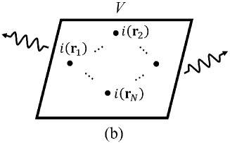
Loaded structures are one approach that allow the formation of any arbitrary current distribution on a surface [23] and to connect this with the discrete feeds required in MIMO antenna design, we can use -port loaded structures [24] as also shown in Fig. 1(b). In this figure, the discrete ports are denoted by black dots [24], [25]. That is the volume is discretized into ports each with currents [25]. By setting the separations between ports in the structure to be significantly less than a wavelength, it can approximate the required current distribution by utilizing appropriate current excitations across the ports. The advantage of this approach is that the feeds for the final potential MIMO antenna are already incorporated at the beginning of the analysis through the -port loaded structure. In the final MIMO antenna design, only some of the ports will be utilized as feeds with the others loaded with reactances to form the required current distribution that achieves the channel capacity bound. This allows us to form antennas with the desired number of feeding ports while achieving performance close to the channel capacity bounds.
For analysis we write as the current at each of the ports in Fig. 1(b). Correspondingly the radiation patterns arising from each of the port currents are written as where is the radiation pattern of the th port excited by a unit current with all the other ports open-circuited, over uniformly sampled three-dimensional (3D) spatial angles. We use these patterns and the results in [31] to decompose the radiation patterns into a natural set of orthonormal modal functions similarly to the Theory of Characteristic Modes (TCM) [24], [32]. These orthonormal modal functions can then be used for analysis of the channel capacity and interpreted as being related to the ADoF of the structure.
For an arbitrary excitation current , the resulting radiation pattern can be expressed as , so that the radiated power is given by
| (1) |
where is the free space impedance, is the correlation of the steering matrix at the transmitter side [31], which is defined as
| (2) |
We can perform eigenvalue decomposition (EVD) on as
| (3) |
where is a real diagonal eigenvalue matrix. It is assumed that there is no inner resonance in the transmit element [24] so that the loaded -port structure can provide orthogonal basis. Therefore, is a positive definite matrix with all eigenvalues being positive . In practice some eigenvalues might be very small and this will affect ADoF as discussed later in the paper. is a unitary matrix whose column vectors , , are eigenvectors of and form a set of current basis. By selecting current to be and collecting the corresponding radiation patterns , , a set of orthogonal radiation patterns can be formed since the inner product of two radiation patterns excited by and is given by
| (4) |
where is the Kronecker delta function (0 if and 1 if ). That is the radiation patterns excited by different column vectors in are orthogonal. The , , can be regarded as the radiation resistance of the th radiation pattern since when excited by (whose norm is unity), the radiated power of is .
The orthonormal basis set with unity radiated power can be written as
| (5) |
so that we have with . The diagonal entries in are scaling factors to form the orthonormal basis. Therefore, for those basis with small radiation resistances, large currents are required to radiate patterns with unity power.
By replicating the approach for the receive volume, we respectively denote the steering matrices of the receive antennas as where , .
The final step is to connect the transmitter and receiver using an appropriate channel model. The beamspace domain or virtual channel representation [26], [33] is a well established approach that decomposes the channel into orthogonal beams. This model fits naturally with the modal decompositions we have formed at the transmitter and receiver. Using the beamspace approach, the equivalent channel matrix in the angular domain can be expressed as
| (6) |
where is the virtual channel whose entries refer to the channel gain from each angle of departure (AoD) to each angle of arrival (AoA) [33]. By taking (6) we can write the overall system model as
| (7) |
where is the additive Gaussian noise and satisfies the complex Gaussian distribution with noise power and is the received signal.
III Channel Capacity Formulation
Using (6) and (7), channel capacity of the system in the beamspace domain can be written as
| (8) |
where is the covariance matrix of current.
We assume the receive antennas ( for tractability) are ideally isolated so that the steering matrix is an exactly orthonormal basis set of receive antennas satisfying . Using (5), we can rewrite the channel matrix (6) as
| (9) |
where with each entry following i.i.d. distribution due to the orthonormality among radiation patterns in and . The capacity (8) is then rewritten using (9) as
| (10) |
Channel capacity is constrained by physical limits consisting of 1) the radiated power constraint with being the upper bound of radiated power and 2) the maximum currents that can exist at the input to the ports of the reactively loaded structure, with being the upper bound of the current norm. In practice, both constraints need to be applied to obtain an implementable antenna. A constraint on the input power (it would be the same as if the antenna was lossless) cannot be formulated since an expression for the input impedances are not known as we do not yet know the final feed arrangement.
In the following subsections, the formulation of capacity with two constraints are derived, which is general and can be applied to arbitrary -port antenna systems.
III-A Capacity with Radiated Power Constraint
We firstly constrain the radiated power for the derivation of channel capacity. This optimization problem can be formulated as
| (11) | ||||
| (12) |
By decomposing arbitrary radiation pattern onto the set of orthonormal radiation pattern basis in , we have
| (13) |
with
| (14) |
so that each entry in refers to the magnitude allocated to each orthonormal pattern basis. The radiated power constraint (12) can be transformed to
| (15) |
where is the covariance matrix of orthonormal pattern basis magnitude. Accordingly, the optimization problem (11) and (12) is re-formulated as
| (16) | ||||
| (17) |
It can be noticed that the problem (16) and (17) is the same as the capacity maximization problem of ideal MIMO. However, due to some extremely small eigenvalues in , the norm of current could be extremely large and not implementable. In other words, the maximum current is unconstrained.
III-B Capacity with Current Constraint
Next, we consider imposing a constraint on the current norm . The optimization problem of channel capacity can then be formulated as
| (18) | ||||
| (19) |
By decomposing the current onto the set of current basis , , we can obtain the coefficient for the decomposition as which refers to the magnitude allocated to the th current basis. We collect the coefficient into a vector which can be related to by
| (20) |
has the same norm as so that the current constraint (19) can be transformed to
| (21) |
where is the covariance matrix of current basis magnitude. Then the problem (18) and (19) can be transformed to
| (22) | ||||
| (23) |
The optimal solution for the currents can be found by performing equal power (EP) or water-filling (WF) allocation directly on .
It can be observed that due to the existence of in (22), the radiated power of each orthogonal basis in is not equal and proportional to the corresponding eigenvalues in . Therefore, in this formulation, the WF method tends to allocate more power to those basis with larger eigenvalues since it increases radiated power and resulting system capacity. In other words, the radiated power is unconstrained.
III-C Capacity with Dual Constraint
Finally, we consider dual constraints imposed by the current norm and radiated power simultaneously. That is, in practical setups the radiated power is limited and the norm of current must also be restricted. This optimization problem is formulated as
| (24) | ||||
| (25) | ||||
| (26) |
We follow the transformation in (14) as well as the formulation in (16) and (17), so the problem (24) to (26) can be transformed to
| (27) | ||||
| (28) | ||||
| (29) |
It can be observed that the capacity formulation is only related to , which is a diagonal matrix with diagonal entries being the eigenvalues of .
To solve the problem (27) to (29), we firstly consider EP allocation method. Although the system provides orthogonal radiation pattern basis, some eigenvalues in are too small so that large currents are required to radiate their corresponding basis (5) which cannot be used for practical MIMO antenna design. To avoid generating large currents, i.e. satisfying the current constraint (29), should be allocated to those basis with largest radiation resistance (i.e. larger eigenvalues in ). Therefore, we equally allocate power to the first basis and drop the remaining basis. These basis can be effectively used with maximum current norm and radiated power , and thus can be regarded as the effective aerial degrees-of-freedom (EADoF) of the transmitter [28].
The diagonal entries in are then given by
| (30) |
The constraint (29) can then be written as
| (31) |
We define in (31) and it can be interpreted loosely as a conductance which has the unit of . In essence for a given , a larger ( high) indicates that the antenna will have a smaller input resistance overall and if it is too small the antenna will not be implementable. Alternatively if is too low ( low), the input impedance will be required to be too high and also not implementable. Therefore we should set it to be in a range centered around 1/50 so that it is in line with the antennas desired input impedance.
Then the EADoF is related to for a fixed SNR as
| (32) |
where the left term refers to the average of the reciprocal of eigenvalues for the first basis. It can be observed from (32) that a larger indicates that the number of available orthogonal basis, i.e. , and the consequent capacity bound can be larger. The maximum can be obtained by solving (32) for a fixed . That is EADoF is dependent on (the maximum allowable current norm given ), indicating the number of basis that can be used with the constraint of current norm and radiation power.
Next we consider using the WF method to maximize capacity in problem (27) to (29). We start with the channel gain of sub-channels in channel matrix . By performing EVD on , we obtain the channel gain matrix which is a real diagonal matrix with , , being the channel gain of the th sub-channel. Then we use the Lagrangian method whose function is given by
| (33) |
where and are Lagrangian multipliers. Taking the partial derivative of with respect to , we have
| (34) |
Combining the solution of in (34), two constraints (28), (29) can be written as [21]
| (35) |
| (36) |
The optimal multipliers and in (36) and (35) can be found via binary search [21] and the optimal can be solved in (34).
It should be noted that the above closed-form expressions for system capacity are formulated without considering the physical realization and practical excitation for MIMO antennas. Therefore, the MIMO antenna structure should be carefully designed and optimized to achieve the capacity bounds with dual constraints, which will be described in the next section.
IV Loaded -port Structure and Analysis
In the previous section, we have provided an optimization formulation to obtain the required port currents on the loaded -port structure for capacity maximization with various constraints. In this section we link those currents to MIMO antenna design with only feeding ports in the loaded -port structures.
IV-A Network Analysis
To begin to construct the MIMO antenna, we divide the -ports in Fig. 1(b) into active feeding ports and loaded ports. The advantage of this approach is that the feeds for the final potential -port MIMO antenna are incorporated at the beginning of the analysis through the -port structure. The equivalent circuit model for the -port network with active feeding ports (numbered 1 to ) and parasitic loaded ports (numbered to ) is shown in Fig. 2. The loaded ports are either lossless with inductive and capacitive reactance or open. The active feeding ports are connected to a matching network to achieve the necessary 50 input impedance. By optimizing the load reactances, we wish to generate orthogonal radiation patterns from the designated feeding ports so that the capacity (8) can be maximized. In essence we will attempt to find loads that create the required current distributions for approaching the capacity bounds. The design procedure for selecting which ports are fed and which are loaded to achieve the optimum channel capacity using (10) is described later.
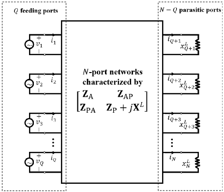
In Fig. 2, the th feeding port is excited by a voltage source , , and the th parasitic port is loaded with reactance , . We group the voltage source excitation , , into a vector as and define as a -dimension zero vector due to there being no excitation at the parasitic ports. We also group current at the feeding and parasitic ports into vectors as and , respectively. The voltage and current in the -port network are then related by
| (37) |
where represents the load reactance connected to each parasitic port. and are the impedance sub-matrix of the feeding ports and the parasitic ports, respectively. and are the sub-matrix referring to the mutual impedance between feeding and parasitic ports with . From (37) we can obtain the relationship between the current on the feeding and parasitic ports as
| (38) |
Our interest is obtaining orthogonal far-field radiation patterns to form the beamspace MIMO system. To that end, we collect the radiation pattern of each feeding port , , in the antenna system into matrix form , which can be given as
| (39) |
where denotes the spatial angle with and representing the elevation and azimuth angles in spherical coordinates, respectively. collects open-circuit radiation patterns of the feeding ports with , being the open-circuit radiation pattern of the th feeding port excited by a unit current when all the other feeding and parasitic ports are open-circuit. Similarly, collects open-circuit radiation patterns of the parasitic ports with , , being the open-circuit radiation pattern of the th parasitic port excited by a unit current when all the other feeding and parasitic ports are open-circuited. It can be observed that consists of the original open-circuit radiation pattern of the feeding ports and a perturbation term affected by the load reactance across the parasitic ports.
We use a full electromagnetic solver, CST studio suite [34], to simulate the open-circuit radiation patterns of all ports of the loaded -port structure. It should be noted that the simulation only needs to be performed once because any radiation pattern excited by any current distribution can then be found by using (39) [35]. This reduces the computation complexity enormously as full electromagnetic simulation is not needed during the load optimization and capacity simulation stages.
IV-B Optimization
To obtain the optimal design of the MIMO antenna, we wish to select active feeding ports and optimize the load reactances at the parasitic ports. The objective is to generate a set of orthogonal radiation patterns in at feeding ports so that the resulting channel capacity can be maximized.
To achieve an optimization result that also meets practical design constraints, we need to note that not all ports would be suitable for use as feeding. For example, ports positioned on the edges of the structure are more likely to be accessible for feeds than those completely surrounded by ports. For this reason, we partition the ports into two sets for optimization. Assume out of ports are feasible feeding ports and whose indices in the set are given by . The objective is therefore to find the optimum ports from the feasible ports where the set of indices for the feeding ports is given by . In addition, we must find the optimum loads for the remaining ports so that together with the unselected feeding ports, the load reactance matrix can meet the requirements of orthogonality for the selected feeding ports.
We use the correlation coefficient between the radiation patterns of two feeding ports, i.e. of the th feeding port and of the th feeding port, to evaluate their similarity, and this is defined as
| (40) |
where satisfies . When , and are orthogonal to each other. Leveraging the correlation coefficient (40), we can formulate the optimization problem as
| (41) |
It should be noted that the optimization variables and are highly coupled with each other in this problem. This is because altering feeding port indices greatly changes the impedance matrix , and in (37), making the problem (41) complicated to solve. To overcome this difficulty and meet these constraints, we propose the use of the alternating optimization method to iteratively optimize the load reactances and selection of the feeding ports [36], [37]. For simplicity, the unselected feeding ports are left open in the entire optimization process to ease the computational burden. However they could also be included in the load optimization process if deemed necessary.
To start with, we randomly select feeding ports, out of , as the initial guess at iteration 0. The set consisting of the indices for initial random feeding ports is given by with being the index of the th initial feeding port. Presetting the unused feeding ports to be open, we then need to optimize load reactances at the parasitic ports where the initial guess for the load reactance matrix is given as with the first diagonal entries being fixed as infinity (open).
At the th iteration, we wish to find the load reactances to produce near orthogonal radiation patterns with feeding ports indices set . This can be performed by solving the optimization problem
| (42) |
This makes the correlation coefficient norm between any two patterns in as close to zero as possible. To solve the unconstrained optimization problem (42), we can use the quasi-Newton method [38] which guarantees convergence to a stationary point of the problem (42). The optimal load reactances at the th iteration are denoted by .
We then use from (42) to optimize the indices of the feeding ports , that is,
| (43) |
which is an NP-hard optimization problem. To solve this problem, we propose a low-complexity approach which is based on sequentially optimizing each entry in , i.e. , ,…, , one-by-one. Specifically, we define as the intermediate state of feeding port indices at the th iteration where the indices of the first feeds have been optimized and the remaining feeds not optimized. When optimizing index for the th feeding port, we fix the other indices and select the optimal from the remaining indices in to minimize the correlation coefficient (40) among all ports in , which can be formulated as
| (44) | ||||
| (45) |
with sequentially taken as . It should be noted that when .
By iteratively optimizing the load reactances and selecting feeding ports, the objective function (42) and (44) can converge to a local optimal solution [37]. Therefore, we obtain the optimal load reactances of the loaded -port structures with feeds with indices of . Algorithm 1 summarizes the overall algorithm for optimizing the load reactances and feeding ports. The performance of the algorithm in finding optimum MIMO antenna configuration will be shown in the next section.
V Numerical Results
In this section, we firstly compare our proposed method with previous work [11] to verify its accuracy and correctness. After that we propose a MIMO antenna that can approach the continuous channel capacity bound.
For channel capacity simulations with the current constraint, we use the same SNR definition as in [11] which is the ratio of the current norm to the noise power . While for capacity simulation with the radiated power constraint and also dual constraints, we use the conventional SNR definition, i.e. the ratio of maximum radiated power to the noise power .
V-A Comparison of Channel Capacity
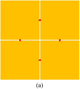
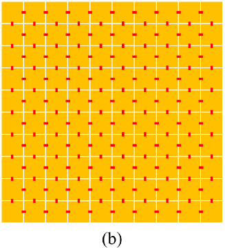
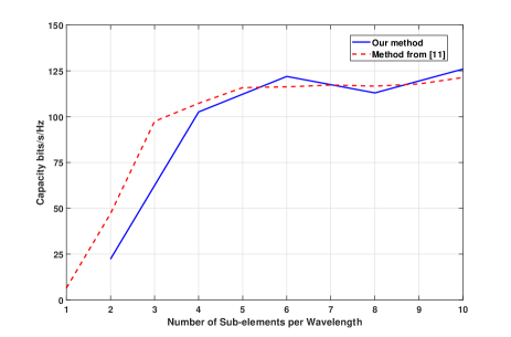
In the first set of simulation results we wish to verify our approach by comparing with previous results [11]. The previous results consider a continuous source current on a 2D square planar surface with one square wavelength size at both the transmitter and receiver. The 2D surface is discretized into an -port structure as shown in Fig 3 where discretizations with 4 and 180 ports are shown. This corresponds to dividing the one wavelength square surface into 4 and 100 sub-elements respectively similarly to the discretizations of previous work [11].
To compare our method to previous work [11], we only need to find the required currents at all ports and do not need to consider finding loads or feeding ports. We can therefore use the results in (22) and (23) directly without considering the loads and feeds to find the port currents.
The same channel setup utilized previously [11] is also invoked and includes single polarization in a rich scattering environment with Rayleigh fading and 2D uniform power angular spectrum (PAS) on the azimuth plane [31]. In addition, we use the current norm constraint so that the capacity optimization problem is formulated as (22) and (23), with WF to find the currents. This is similar to equation (21) in [11].
Simulation results of the system capacity are shown in Fig. 4 for various levels of discretizations. In the figure the number of discretizations per dimension is used to align with previous work [11]. That is 10 sub-elements per wavelength correspond to 100 sub-elements in total. It can be observed that by using our method, the system capacity approaches that using the method in [11] when the number of sub-elements per wavelength is more than four. The capacity gap (for 4 or less sub-elements per square wavelength) arises due to the current on the discrete ports being an approximation to the continuous current on the surface, which is related to the position of the ports in the -port structure. Therefore, we can conclude that our method can obtain the continuous-space electromagnetic channel capacity bound if the dimension of the sub-element and the separation distance between ports is less than a wavelength (from Fig. 3 greater than 5 sub-elements per wavelength).
V-B MIMO Antenna Capacity Bound
Next, we use the technique in Section IV to design a practical MIMO antenna that approaches the capacity bounds. The frequency considered in the following is 2.4 GHz so that the wavelength is 125 mm.
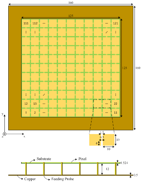
The first step is to propose a structure that is implementable with feeds but general enough to allow the formation of arbitrary current distributions for capacity maximization. As such our proposed -port structure is shown in Fig. 5 where a 2D square copper planar surface with one square wavelength size is again utilized. The copper surface is mounted on a substrate where the copper has electric conductivity of S/m while the substrate is made with Rogers 5880C which has permittivity of 2.2 and loss tangent of 0.0009. We discretize the 2D copper surface into a sub-element array where the size of the sub-element is . To implement the feeds, an additional copper plane is placed underneath as a ground plane so that a conventional feed can be connected between the ground and the center of a sub-element as shown in the elevation view in Fig. 5. The ports of the structure are defined as the ports across each pair of adjacent sub-elements on the surface and also between the ground and the center of each sub-element. That is there are 220 ports on the surface and 121 ports between the ground and sub-elements making up a total of ports. The feeding ports need to be selected from the 121 ports between the ground and sub-elements.
While the ultimate aim is to select feeding ports from the ground to sub-element ports, we firstly need to find the required currents on the ports to optimize capacity and approach the capacity bounds similarly as in Section V.A. This allows us to first determine the capacity performance of the structure with ideal port currents. The final load reactances and feeds arrangements of the antenna that can approximate these currents are found in the next subsection.
In the capacity simulations, we obtain them as a function of (, etc.) basis with the highest eigenvalues (out of for transmission. This allows us to determine the number of EADoF provided by the structure. In the simulations, we use ideally isolated antennas at the receiver side. We also assume a rich scattering environment so that entries in satisfy for . In addition, dual polarization in a rich scattering environment with Rayleigh fading and 3D uniform PAS over full sphere is utilized. For these reasons the capacity results obtained for this channel will be much greater than that obtained in Section V.A which used only one polarization, a 2D PAS and a receiver antenna that was the same as the transmitter.
V-B1 Capacity Bound with Individual Constraints
We simulate the capacity of the proposed structure when we use the basis functions with the highest eigenvalues to create a system with the two individual constraints of current norm and radiated power. The simulated capacity with the two constraints using EP allocation and WF method are shown in Fig. 6. These are benchmarked with the results of an ideal MIMO system where the transmitter is equipped with spatially isolated antennas. It can be observed that if we only consider the constraint of radiated power, the simulated capacity of the structure is the same as that of ideal MIMO. However, the current norm in this case can be extremely large and not implementable.
On the other hand, if we only consider the constraint of current norm, the capacity of the loaded structure is higher than the ideal MIMO systems for the first few basis. This is because those basis with large eigenvalues have larger radiated power than the ideal MIMO system. However, when we consider more basis, e.g. more than 50, the increase in capacity is negligible since those basis have small eigenvalues and only radiate limited power. Therefore, in this case the WF method can allocate more power to these 50 basis with large eigenvalues to improve the capacity.
V-B2 Capacity Bound with Dual Constraint
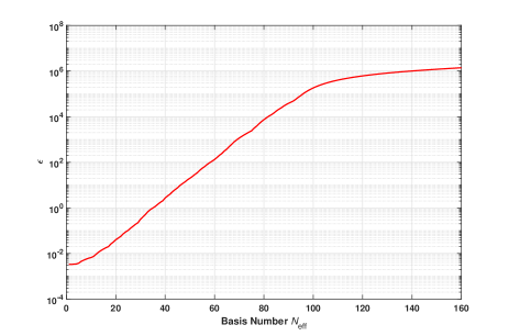
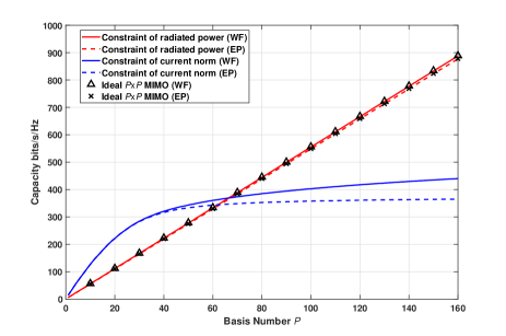
Next we consider imposing dual constraints for the simulation of channel capacity and this leads us to consider and . In Fig. 7, we plot the minimum for the first basis as calculated in (32). It can be noticed that is an increasing function of as expected.
For an ideal lossless antenna, the input impedance is , i.e. . Therefore a region of interest on Fig. 7, is when . In this region is approximately 18 and therefore provides an estimate of the minimum EADoF to expect. In essence we can expect to achieve at least 18 ports in the one square wavelength area. We consider it as a lower bound in practice, depending on the exact relation between and . We may be able to achieve more ports because the internal currents in the antenna can be higher than those at the feeds.
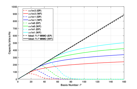
In Fig. 8 we plot the resulting capacity when we use the first basis functions to create a system for various using EP and WF. It can be observed again that the capacity of the MIMO system using the -port structure increases as becomes larger. When considering basis smaller than , the system capacity of MIMO using the loaded structure is the same as that of ideal MIMO. However when approaches , the capacity using EP allocation starts to decrease since equality in dual constraints cannot be achieved. The WF method allocates most power to the first basis so that the capacity slightly increases when adding more basis to the MIMO system. In addition, the value points where the WF and EP lines separate indicate the number of available basis (i.e. EADoF) provided by the value structure as calculated in (32) and approximately match with the results in Fig. 7.
The results in Fig. 7 and and Fig. 8 are useful references in designing MIMO antenna for approaching the capacity bound. The use of provides us with an estimate of the number of feeding ports or . In particular, we can expect to be able to provide at least 18 ports in the one square wavelength size antenna structure shown in Fig. 5.
V-C MIMO Antenna Design
To provide a useful antenna, we need to select feeding ports and the loads for all the ports in the -port loaded structure. The feeding ports and loads must be selected to achieve a close match to the optimum currents found in the previous section for a feasible . This then would provide the optimum antenna configuration that can achieve the channel capacity bound with dual constraints.
As discussed previously for an ideal lossless antenna, the input impedance is and therefore so that is at least 18. Expecting to have higher currents internally on the antenna, we aim for 20 ports in our design. That is we will need to re-create the currents obtained when from the previous section.
To reduce the computational effort in finding the loads, we preset the sub-elements in the center row and center column of the 2D copper surface as being connected together (shorted) so there is a single large cross element centered on the surface. That is ports {56, 57, 58, 59, 60, 61, 62, 63, 64, 65, 66, 6, 17, 28, 39, 50, 72, 83, 94, 105, 116} in Fig. 5 are shorted together. The cross element separates the other sub-elements into four sub-square arrays. The cross is also isolated from the other sub-elements so that the ports between the cross and the other adjacent sub-elements are open without loads. In effect, we are presetting some of the ports to be shorted or open on the surface. This reduces the computational load of the optimization by reducing the number of load reactances to be found from 220 to 160. In addition, to reduce the search space for the feeds we also restrict it to the ports between the ground plane and the sub-elements on the edge of each sub-square array (instead of all 121 possible locations). For those ports underneath the surface that were not selected as feeds, we set them to be open.
To find the optimum reactances across the 160 ports on the surface and the indices of the 20 feeding ports underneath, we use the method as described in Section IV so that the excited radiation patterns of the 20 feeding ports are closest to being orthogonal (42). The final indices of the 20 feeding ports after the alternating optimization are given by
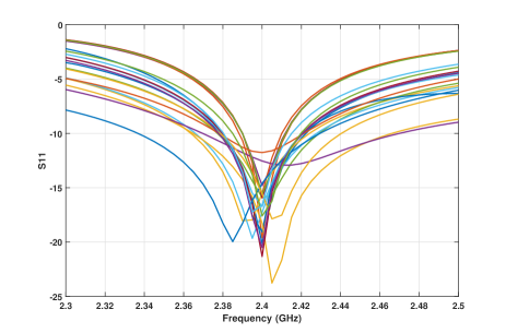
and their physical location can be found from Fig. 5. The 20 feeding ports are then each fed by a feeding probe across the common ground and the center of the selected sub-elements as shown in the elevation view in Fig. 5. The impedance matching for the 20 feeding ports is performed separately with a conventional T-type matching network to achieve matching to 50 . The return loss (S11) results of the 20 ports are provided in Fig. 9 where the reflected power at 2.4 GHz is around -15 dB and the bandwidth is around 40 MHz.
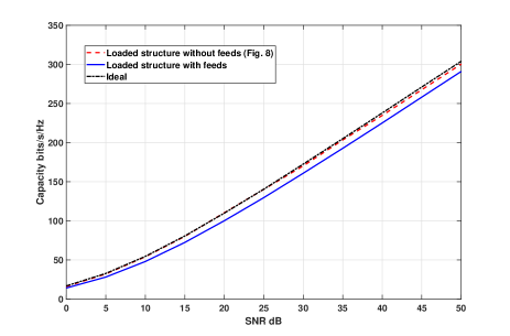
By using the 20 excited radiation patterns from the resultant loaded structure with 20 feeds, and a beamspace channel model (7), the capacity of the MIMO system is found and the simulated results are shown in Fig. 10. These are also benchmarked with the capacity bound of the loaded structure without feeds obtained by WF method in Section III.C and the capacity of ideal MIMO. It can be observed that the MIMO antenna using the loaded structure with 20 feeds achieves performance close to ideal MIMO and the capacity bound predicted by Fig. 8 for loaded structure without feeds. The capacity gap is due to the small correlations among the radiation patterns of the feeding ports and power loss from mutual coupling. However, the key advantage of the proposed method is that the optimum antenna structure for the MIMO transmitter with size constraint can be found with only minor compromise on system capacity.
VI Conclusion
In this paper, we have proposed a novel method for designing antennas that approach the continuous-space electromagnetic channel capacity bounds. The method can link continuous-space electromagnetic channel capacity bounds to MIMO antenna design. The method is not restricted to a specific antenna configuration and uses loaded -port structures to discretize the continuous space and represent arbitrary antenna geometries. It is useful for designing compact MIMO antennas that can approach channel capacity bounds when constrained by size.
In the proposed method, we derive the closed-form expressions for the channel capacity limits using a beamspace channel model with a current constraint, radiated power constraint as well as with dual constraints. We also introduce a method for antenna design using the loaded ports structure and provide an efficient alternating optimization approach for finding the optimum MIMO antenna configuration to generate orthogonal radiation patterns. This can be used to construct a beamspace MIMO system that approaches the channel capacity bounds.
Simulation results of the channel capacity using our proposed method matches well with previous work. Furthermore, by optimizing the load reactance and feeding port positions in our proposed antenna design with one square wavelength size, the achieved capacity performance is close to the continuous-space channel capacity bounds, demonstrating the effectiveness of the proposed method. In particular we show that at least 18 ports can be supported in a one wavelength square structure to achieve the continuous-space electromagnetic channel capacity bound. It is also shown that the limit on the number of ports is constrained by the maximum current that the antenna can handle. An example design for a 20-port antenna in a one square wavelength area that achieves the capacity bounds is also provided. One challenge of the final antenna is the limited bandwidth and this can be addressed by increasing the height in the antenna design.
References
- [1] C. E. Shannon, “A mathematical theory of communication,” The Bell system technical journal, vol. 27, no. 3, pp. 379–423, 1948.
- [2] V. Tarokh, N. Seshadri, and A. Calderbank, “Space-time codes for high data rate wireless communication: performance criterion and code construction,” IEEE Trans. Inf. Theory, vol. 44, no. 2, pp. 744–765, 1998.
- [3] E. Telatar, “Capacity of multi-antenna Gaussian channels,” Eur. Trans. Telecommun., vol. 10, no. 6, pp. 585–595, 1999.
- [4] D. M. Pozar, Microwave engineering. John wiley & sons, 2011.
- [5] C. A. Balanis, Antenna theory: analysis and design. John wiley & sons, 2015.
- [6] M. D. Migliore, “On electromagnetics and information theory,” IEEE Trans. Antennas and Propagation, vol. 56, no. 10, pp. 3188–3200, 2008.
- [7] F. K. Gruber and E. A. Marengo, “New aspects of electromagnetic information theory for wireless and antenna systems,” IEEE Trans. Antennas Propag., vol. 56, no. 11, pp. 3470–3484, 2008.
- [8] O. M. Bucci and G. Franceschetti, “On the degrees of freedom of scattered fields,” IEEE Trans. Antennas Propag., vol. 37, no. 7, pp. 918–926, 1989.
- [9] A. S. Poon, R. W. Brodersen, and D. N. Tse, “Degrees of freedom in multiple-antenna channels: A signal space approach,” IEEE Trans. Inf. Theory, vol. 51, no. 2, pp. 523–536, 2005.
- [10] M. D. Migliore, “On the role of the number of degrees of freedom of the field in MIMO channels,” IEEE Trans. Antennas Propag., vol. 54, no. 2, pp. 620–628, 2006.
- [11] M. A. Jensen and J. W. Wallace, “Capacity of the continuous-space electromagnetic channel,” IEEE Trans. Antennas Propag., vol. 56, no. 2, pp. 524–531, 2008.
- [12] W. Jeon and S.-Y. Chung, “Capacity of continuous-space electromagnetic channels with lossy transceivers,” IEEE Trans. Inf. Theory, vol. 64, no. 3, pp. 1977–1991, 2017.
- [13] R. D. Murch and K. B. Letaief, “Antenna systems for broadband wireless access,” IEEE Commun. Mag., vol. 40, no. 4, pp. 76–83, 2002.
- [14] C.-Y. Chiu, J.-B. Yan, and R. D. Murch, “Compact three-port orthogonally polarized MIMO antennas,” IEEE Antennas Wirel. Propag. Lett., vol. 6, pp. 619–622, 2007.
- [15] J. Ren, W. Hu, Y. Yin, and R. Fan, “Compact printed MIMO antenna for UWB applications,” IEEE Antennas Wirel. Propag. Lett., vol. 13, pp. 1517–1520, 2014.
- [16] G. Zhai, Z. N. Chen, and X. Qing, “Enhanced isolation of a closely spaced four-element MIMO antenna system using metamaterial mushroom,” IEEE Trans. Antennas Propag., vol. 63, no. 8, pp. 3362–3370, 2015.
- [17] L. Lu, G. Y. Li, A. L. Swindlehurst, A. Ashikhmin, and R. Zhang, “An overview of massive MIMO: Benefits and challenges,” IEEE J. Sel. Top. Signal Process., vol. 8, no. 5, pp. 742–758, 2014.
- [18] S. Soltani and R. D. Murch, “A compact planar printed MIMO antenna design,” IEEE Trans. Antennas Propag., vol. 63, no. 3, pp. 1140–1149, 2015.
- [19] S. Shen and R. D. Murch, “Impedance matching for compact multiple antenna systems in random RF fields,” IEEE Trans. Antennas Propag., vol. 64, no. 2, pp. 820–825, 2015.
- [20] J. W. Wallace and M. A. Jensen, “Mutual coupling in MIMO wireless systems: A rigorous network theory analysis,” IEEE Trans. Wirel. Commun., vol. 3, no. 4, pp. 1317–1325, 2004.
- [21] L. Sun, P. Li, M. R. McKay, and R. D. Murch, “Capacity of MIMO systems with mutual coupling: Transmitter optimization with dual power constraints,” IEEE Trans. Signal Process., vol. 60, no. 2, pp. 848–861, 2011.
- [22] V. Shyianov, M. Akrout, F. Bellili, A. Mezghani, and R. W. Heath, “Achievable rate with antenna size constraint: Shannon meets Chu and Bode,” IEEE Trans. Commun., 2021.
- [23] R. Harrington and J. Mautz, “Control of radar scattering by reactive loading,” IEEE Trans. Antennas Propag., vol. 20, no. 4, pp. 446–454, 1972.
- [24] J. Mautz and R. Harrington, “Modal analysis of loaded N-port scatterers,” IEEE Trans. Antennas Propag., vol. 21, no. 2, pp. 188–199, 1973.
- [25] R. Harrington and J. Mautz, “Pattern synthesis for loaded n-port scatterers,” IEEE Trans. Antennas Propag., vol. 22, no. 2, pp. 184–190, 1974.
- [26] A. M. Sayeed, “Deconstructing multiantenna fading channels,” IEEE Trans. Signal Process., vol. 50, no. 10, pp. 2563–2579, 2002.
- [27] V. I. Barousis, A. G. Kanatas, and A. Kalis, “Beamspace-domain analysis of single-RF front-end MIMO systems,” IEEE Trans. Veh. Technol., vol. 60, no. 3, pp. 1195–1199, 2011.
- [28] V. Barousis and A. G. Kanatas, “Aerial degrees of freedom of parasitic arrays for single RF front-end MIMO transceivers,” Progress Electromagn. Research, vol. 35, pp. 287–306, 2011.
- [29] A. Kalis, A. G. Kanatas, and C. B. Papadias, “A novel approach to MIMO transmission using a single RF front end,” IEEE J. Sel. Areas Commun., vol. 26, no. 6, pp. 972–980, 2008.
- [30] O. N. Alrabadi, C. B. Papadias, A. Kalis, and R. Prasad, “A universal encoding scheme for MIMO transmission using a single active element for PSK modulation schemes,” IEEE Trans. Wirel. Commun., vol. 8, no. 10, pp. 5133–5142, 2009.
- [31] Z. Han, S. Shen, Y. Zhang, C.-Y. Chiu, and R. Murch, “A pattern correlation decomposition method for analysis of ESPAR in single-RF MIMO systems,” IEEE Trans. Wirel. Commun., 2021.
- [32] Z. Han, Y. Zhang, S. Shen, Y. Li, C.-Y. Chiu, and R. Murch, “Characteristic mode analysis of ESPAR for single-RF MIMO systems,” IEEE Trans. Wirel. Commun., vol. 20, no. 4, pp. 2353–2367, 2021.
- [33] K. Maliatsos and A. G. Kanatas, “Modifications of the IST-WINNER channel model for beamspace processing and parasitic arrays,” in in Proc. 7th Eur. Conf. Antennas and Propag. IEEE, 2013, pp. 989–993.
- [34] CST Microwave Studio 2019, http://www.cst.com.
- [35] Y. Zhang, S. Shen, Z. Han, C.-Y. Chiu, and R. Murch, “Compact MIMO systems utilizing a pixelated surface: Capacity maximization,” IEEE Trans. Veh. Technol., vol. 70, no. 9, pp. 8453–8467, 2021.
- [36] Y. Bingbing, R. Wenbo, Y. Bolin, and L. Yang, “An indoor positioning algorithm and its experiment research based on RFID,” International Journal on Smart Sensing & Intelligent Systems, vol. 7, no. 2, 2014.
- [37] J. C. Bezdek and R. J. Hathaway, “Convergence of alternating optimization,” Neural, Parallel & Scientific Computations, vol. 11, no. 4, pp. 351–368, 2003.
- [38] P. E. Gill and W. Murray, “Quasi-Newton methods for unconstrained optimization,” IMA J. Appl. Math., vol. 9, no. 1, pp. 91–108, 1972.