Using parallel computation to improve Independent Metropolis–Hastings based estimation
Abstract
In this paper, we consider the implications of the fact that parallel raw-power can be exploited by a generic Metropolis–Hastings algorithm if the proposed values are independent from the current value of the Markov chain. In particular, we present improvements to the independent Metropolis–Hastings algorithm that significantly decrease the variance of any estimator derived from the MCMC output, at a null computing cost since those improvements are based on a fixed number of target density evaluations that can be produced in parallel. The techniques developed in this paper do not jeopardize the Markovian convergence properties of the algorithm, since they are based on the Rao–Blackwell principles of Gelfand and Smith (1990), already exploited in Casella and Robert (1996), Atchadé and Perron (2005) and Douc and Robert (2011). We illustrate those improvements both on a toy normal example and on a classical probit regression model, but stress the fact that they are applicable in any case where the independent Metropolis–Hastings is applicable.
Keywords: MCMC algorithm, independent Metropolis–Hastings, parallel computation, Rao-Blackwellization, permutation.
1 Introduction
The Metropolis–Hastings (MH) algorithm provides an iterative and converging scheme to sample from a complex target density . Each iteration of the algorithm generates a new value of the Markov chain that relies on the result of the previous iteration. The underlying Markov principle is well-understood and leads to a generic convergence principle as described, e.g., in Robert and Casella (2004). However, due to its Markovian nature, this algorithm is not straightforward to parallelize, which creates difficulties in slower languages like R (R Development Core Team, 2006). Nevertheless, the increasing number of parallel cores that are available at a very low cost drives more and more interest in “parallel-friendly” algorithms, that is, in algorithms that can benefit from the available parallel processing units on standard computers (see. e.g., Holmes et al. (2011), Lee et al. (2009), Suchard et al. (2010)).
Different techniques have already been used to enhance some degree of parallelism in generic Metropolis–Hastings (MH) algorithms, beside the basic scheme of running MCMC algorithms independently in parallel and merging the results. For instance, a natural entry is to rely on renewal properties of the Markov chain (Mykland et al., 1995, Robert, 1995, Hobert et al., 2002), waiting for all chains to exhibit a renewal event and then using the blocks as iid, but the constraint of Markovianity cannot be removed. Rosenthal (2000) also points out the difficult issue of accounting for the burn-in time: while, for a single MCMC run, the burn-in time is essentially negligible, it does create a significant bias when running parallel chains (unless perfect sampling can be implemented). Craiu and Meng (2005) mix antithetic coupling and stratification with perfect sampling. Using a different approach, Craiu et al. (2009) rely on parallel chains to build an adaptive MCMC algorithm, considering in essence that the product of the target densities over the chains is their target, a perspective that obviously impacts the convergence properties of the multiple chain. Corander et al. (2006) take advantage of parallelization to build a non-reversible algorithm that can avoid the scaling effect of specific neighborhood structures, hence focussing on a very special type of problem.
A particular family of MH algorithm is the Independent Metropolis–Hastings (IMH) algorithm, where the proposal distribution (and hence the proposed value) does not depend on the current state of the Markov chain. Due to this characteristic, this specific algorithm is easier to parallelize and can therefore be considered as a good building block toward efficient parallel Markov Chain Monte Carlo algorithms, as will be explained in Section 2. We will focus on cases where the computation of the likelihood function constitutes the major part of the execution time in the MH algorithm. A most realistic example of this setting is provided in Wraith et al. (2009), where the model is based on a very complex Fortran program translating the results of several cosmological experiments, hence highly demanding in computing time. In this model, Wraith et al. (2009) use adaptive importance sampling and massive parallelization, rather than MCMC.
The fundamental idea in the current paper is that one can take advantage of the parallel abilities of arbitrary items of computing machinery, from cloud computing to graphical cards (GPU), in the case of the generic IMH algorithm, producing an output that corresponds to a much improved Monte Carlo approximation machine at the same computational cost. The techniques presented here are related with those explained in Perron (1999) and more closely to those in Atchadé and Perron (2005, Section 3.1), since these authors condition upon the order statistic of the values proposed by the IMH algorithm, although in those earlier papers the links with parallel computation were not established and hence the implementation of the Rao-Blackwellization scheme became problematic for long chains.
The plan of the paper is as follows: the standard IMH algorithm is recalled in Section 2, followed by a description of our improving scheme, called here “block Independent Metropolis–Hastings” (block IMH). This improvement depends on a choice of permutations on that is described in details in Section 3. We demonstrate the connections between block IMH and Rao–Blackwellization in Section 4. Results for a toy example are presented throughout the paper and a realistic probit regression example is described in Section 5 as an illustration of the method.
2 Improving the IMH algorithm
2.1 Standard IMH algorithm
We recall here the basic IMH algorithm, assuming the availability of a proposal distribution that we can sample, and which probability density is known up to a normalization constant. The independent Metropolis–Hastings algorithm, described in Algorithm 1, generates a Markov chain with invariant density , corresponding to the target distribution.
In the larger picture of Monte Carlo and MCMC algorithms, the IMH algorithm holds a rather special status. It has certainly been studied more often than other MCMC schemes (Robert and Casella, 2004), but it is undoubtedly a less practical solution than the more generic random walk Metropolis–Hastings algorithm. For instance, it is rather rarely used by itself because it requires the derivation of a tolerably good approximation to the true target, approximation that most often is unavailable. On the other hand, first-order approximations and Metropolis-within-Gibbs schemes are not foreign to calling for IMH local moves based on Gaussian representations of the targets. The reason theoretical studies of the IMH algorithm abound is that it has strong links with the non-Markovian simulation methods such as importance sampling. Contrary to random-walk Metropolis–Hastings schemes, IMH algorithms may enjoy very good convergence properties and may also reach acceptance probabilities that are close to one. Furthermore, the potentially large gain in variance reduction provided by the parallelization scheme developped in this paper may counteract the lesser efficiency of the original IMH compared with the random walk Metropolis–Hastings algorithm.
An important feature of the IMH algorithm, when addressing parallelism, is that it cannot work but in an iterative manner, since the outcome of step , namely the value , is required to compute the acceptance ratio at step . This sequential construction is compulsory for the validation of the algorithm given the Markov property at its core (Robert and Casella, 2004). Nonetheless, given that, in the IMH algorithm, the proposed values are generated independently from the current state of the Markov chain, , it is altogether possible to envision the generation of proposed values first, along with the computation of the associated ratios . Once this computation requirement is completed, only the acceptance steps need to be considered iteratively. This two-step perspective makes for a huge saving in computing time when the simulation of the ’s and the derivation of the ’s can be achieved in parallel since both the remaining computation of the ratios given the ’s and their subsequent comparison with uniform draws typically are orders of magnitude faster.
In this respect the IMH algorithm strongly differs from the random walk Metropolis–Hastings (RWMH) algorithm, for which acceptance ratios cannot be processed beforehand because the proposed simulated values depend on the current value of the Markov chain. The universal availability of parallel processing schemes may thus lead to a new surge of popularity for the IMH algorithm. Indeed, when taking advantage of parallel processing units, an IMH can be run for times as many iterations as RWMH, at almost the same computing cost since RWMH cannot be directly parallelized.
In order to better describe this increased computing power, we first note that, once successive values of a Markov chain have been produced, the sequence is usually processed as a regular Monte Carlo sample to obtain an approximation of an expectation under the target distribution, say, for some arbitrary functions . We propose in this paper a technique that improves the precision of the estimation of this expectation by taking advantage of parallel processing units without jeopardizing the Markov property.
Before presenting our improvement scheme, we introduce the notation (read “or”) for the operator that represents a single step of the IMH algorithm. Using this notation, given the current value and a sequence of independent proposed values , the IMH algorithm goes from step to step according to the diagram in Figure 1.

2.2 Block IMH algorithm
We propose to take full advantage of the simulated proposed values and of the computation of their corresponding ratios. To this effect, we introduce the block IMH algorithm, made of successive simulations of blocks of size . In this alternative scheme, the number of blocks is such that the number of desired iterations is equal to , in order to keep the comparison with a standard IMH output fair. Usually needs not be calibrated since it represents the number of physical parallel processing units that can be exploited by the code. However, in principle, this number can be set arbitrarily high and based on virtual parallel processing units, the drawback being then an increase in the computing cost. (Note that the block IMH algorithm can also be implemented with no parallel abilities, still it provides a gain in variance that may counteract the increase in time.) In the following examples, we take varying from to . We first explain how a block is simulated, and then how to move from one block to the next.
A block consists in the generation of parallel generations of values of Markov chains, all starting at time from the current state and all based on the same proposed simulated values . The different between the floes is the orders in which those ’s are included. For instance, these orders may be the circular permutations of , or they may be instead random permutations, as discussed in detail (and compared) in Section 3. The block IMH algorithm is illustrated in Figure 2 for the circular set of permutations.

It should be clear that each of the parallel chains found in this block is a valid MCMC sequence of length when taken separately. As such, it can be processed as a regular MCMC output. In particular, if is simulated from the stationary distribution, any of the subsequent is also simulated from the stationary distribution. However, the point of the parallel flows is double:
-
•
it aims at integrating out part of the randomness resulting from the ancillary order in which the ’s are chosen, getting close to the conditioning on the order statistics of the ’s advocated by Perron (1999);
-
•
it also aims at partly integrating out the randomness resulting from the generation of uniform variables in the selection process, since the block implementation results in drawing uniform realizations instead of uniform realizations for a standard IMH setting.
Both of those points essentially amount to implementing a new Rao–Blackwellization technique (a more precise connection is drawn in Section 4). In an independent setting, each of the ’s occurs a number of times across the steps of the parallel chains, i.e. for a number of realizations. Therefore, when considering the standard estimator of , based on a single MCMC chain,
this estimator necessarily has a larger variance than the double average
where and is the number of times is repeated. (The proof for the reduction of the variance from to easily follows from a double integration argument.) We again insist on the compelling feature that computing using parallel processing units does not cost more time than computing using a single processing unit.

In order to preserve its Markov validation, the algorithm must properly continue at time . An obvious choice is to pick one of the sequences at random and to take the corresponding as the value of , starting point of the next parallel block. This mechanism is represented in Figure 3. While valid from a Markovian perspective, since the sequences are marginally produced by a regular IMH algorithm, this means that the chain deduced from the block IMH algorithm is converging at exactly the same speed as the original IMH algorithm. An alternative choice for the starting points of the blocks takes advantage of the weights on the ’s that are computed via the block structure. Indeed, those weights essentially act as importance weights and they allow for a selection of any of the ’s as the starting point of the incoming block, which corresponds to choosing one of the proposed ’s with probability proportional to . While this proposal does reduce the length of the resulting chain, it does not impact the estimation aspects (which still involve all of the values) and it could improve convergence, given that the weighted ’s behave like a discretized version of a sample from the target density . We will not cover this alternative any further.
The original version of the block IMH algorithm is described in Algorithm 2, The algorithm is made of a loop on the blocks and an inner loop on the parallel chains of each block. The steps of this inner loop are actually meant to be implemented in parallel. The output of Algorithm 2 is double:
- •
-
•
a array , on which the estimator is based.
-
•
-
•
proposed values shuffled with the permutation
-
•
the corresponding ratios ’s
2.3 Savings on computing time
Since the point-wise evaluation of the target density is usually the most computer-intensive part of the algorithm, sampling additional uniform variables has a negligible impact here, as do further costs related to the storage of vectors larger than in the original IMH. This is particularly compelling since the multiple chains do not need to be stored further than during a single block execution time. That is why, although we sample times more uniforms in the block IMH algorithm, we still consider it to be running at roughly of the same cost as the IMH algorithm. The number of target density evaluations indeed is the same for both and most often represent the overwhelming part of the computing time in the Metropolis–Hastings algorithm. Besides, pseudo-random generation of uniforms can also benefit from parallel processing, see e.g. L’Ecuyer et al. (2001).
In the following Monte Carlo experiment, various versions of the block IMH algorithm are compared one to another, as well as to standard IMH and importance sampling. We stress that a straightforward reason for not conducting a comparison with a plain parallel algorithm based on independent parallel chains is that it does not make much sense cost-wise. Indeed, running parallel MCMC chains of the same length does cost times more in terms of target density evaluations. Obviously, if one insists on running independent chains, for instance as to initialize an MCMC algorithm from several well-dispersed starting points, each of those chains can benefit from our stabilizing method, which will improve the resulting estimation.
The method is presented here for square blocks of dimension , but blocks could be rectangular as well: the algorithm is equally valid when using permutations, leading to blocks. We focus here on square blocks because when the machine at hand provides parallel processing units, then it is most efficient to simulate the proposed values and the uniforms, and to compute the target densities and the acceptance ratios at the proposed values in parallel. Once again, the block IMH algorithm with square blocks has about the same cost as the original IMH algorithm, because computing target densities and acceptance ratios does more than compensate for the cost of randomly picking an index at the end of each block. This amounts to say that line 4 of Algorithm 1 and line 5 of Algorithm 2 are (by far) the most computationally demanding ones in the respective algorithms.
2.4 Toy example
We now introduce a toy example that we will follow throughout the paper. The target is the density of the standard normal distribution and the proposal is the density of the Cauchy distribution. Hence, the density ratio is
We only consider the integral , the mean of equal to zero in this case. The acceptance rate of the IMH algorithm for this example is around . (Note that IMH with higher acceptance rates are considered to be more efficient, in opposition to other Metropolis–Hastings algorithms, see Robert and Casella, 2004.)
In all results related to the toy example presented thereafter, independent runs are used to compute the variance of the estimates. The value of represents the number of parallel processing units that are available, ranging from for a desktop computer to for a cluster or a graphics processing unit (GPU) (this value could even be larger for computers equipped with multiple GPUs).
The results of the simulation experiments are presented in Figures 4–8 as barplots, which indicate the percentage of variance decrease associated with the estimators under comparison, the reference estimator being the standard IMH output . In agreement with the block sampling perspective, the same proposed values and uniform draws were used for all the estimators that are plotted on the same graph (that is, for a given value of ), so that the comparison is not perturbed by an additional noise associated with the simulation.
3 Permutations
While the choice of permutations in line 7 of Algorithm 2 is irrelevant for the validation of the parallelization, it has important consequences on the variance improvement and we now discuss several natural choices. The idea of testing various orders of the proposed values in a IMH algorithm appeared in Atchadé and Perron (2005) where the permutations were chosen to be circular. We first list natural types of permutations along with some justifications, and then we empirically compare their impact on estimation performances for the toy example.
3.1 Five natural permutations
Let be the set of permutations of . Its size is , therefore too large to allow for averaging over all permutations, although this solution would be ideal. We consider the simpler option of finding efficient permutations in , denoted by , the goal being a choice favoring the largest possible decrease in the variance of the estimator defined in Section 2.
3.1.1 Same order
The most basic choice is to pick the same permutation on each of the chains:
This selection may sound counterproductive, but we still obtain a significant decrease in the variance of using this set of permutations, when compared with . The reason for the improvement is that times more uniforms are used in than in , leading to a natural Rao-Blackwellization phenomenon that is studied in details in Section 4. Nonetheless this simplistic set of permutations is certainly not the best choice since it does not integrate out the ancillary randomness resulting from the arbitrary ordering of the proposed values.
3.1.2 Circular permutations
Another simple choice is to use circular permutations. For , we define
An appealing property of the circular permutations is that each simulated value is proposed and evaluated at a different step for each chain. However, a drawback is that the order is not deeply changed: for instance will always be proposed one step before except for one of the chains, for which is proposed first.
3.1.3 Random permutations
A third choice is to use random orders, that is random shufflings of the sequence . We can either draw those random permutations with or without replacement in the set , but considering the cardinality of the set this does not make a large difference. Indeed, it is unlikely to draw twice the same permutation, except for very small values of .
3.1.4 Half-random half-reversed permutations
A slightly different choice of permutations consists in drawing permutations at random ( is taken to be even here to simplify the notations). Then, denoting the first permutations by , we define for :
The motivation for this inversion of the orders is that, in the second half of the permutations, the opposition with the “reversed” first half is maximal. This choice, suggestion of Art Owen (personal communication), aims at minimizing the possible common history among the parallel chains. Indeed two chains with the same proposed values in reverse order cannot have a common path of length more than 1.
3.1.5 Stratified random permutations
Finally we can try to draw permutations that are far from one another in the set . For instance we can define the lexicographic order on , draw indices from a low discrepancy sequence on the set and select the permutations corresponding to these indices. In a simpler manner, we do use here a stratified sampling scheme: we first draw a random permutation conditionally on its first element being , then another permutation beginning with , and so forth until the last permutation which begins with .
3.2 A Monte Carlo comparison
We compare the five described types of permutations on the toy example. Figure 4 shows the results for various values of , displaying the variance reduction of associated with each of the permutation orders, compared to the variance of the original IMH estimator . For each of the independent replications, the block IMH algorithm was launched on one single block, e.g. with using the notation of Section 2, since plays no role whatsoever in this comparison.
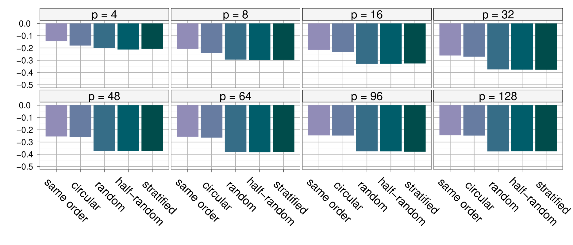
As mentioned above, using the same order in the ’s for each of the parallel chains already produces a significant decrease of about in the variance of the estimators. This simulation experiment shows that the three random permutations (random, half-random half-reversed and stratified) are quite equivalent in terms of variance improvement and that they are significantly better than the circular permutation proposal, which only slightly improves over the “same order” scheme. Therefore, in the next Monte Carlo experiments, we will only use the random order solution, simplest of the random schemes. An amount of improvement like when is quite impressive when considering that it is essentially obtained cost-free for a computer with parallel abilities (Holmes et al., 2011).
4 Rao–Blackwellization
Another generic improvement that can be brought over classical MH algorithms is Rao–Blackwellization (Gelfand and Smith, 1990, Casella and Robert, 1996). In this section, two Rao–Blackwellization methods are presented, one that is computationally free and one that, on the contrary, is computationally expensive. We then implement both solutions within the block IMH algorithm and explain why the “same order” scheme already improves upon the IMH algorithm.
4.1 Primary Rao–Blackwellization
Within the standard IMH algorithm of Section 2.1, a cost-free improvement can be obtained by a straightforward Rao–Blackwellization argument. Given that at step , is accepted with probability and rejected with probability , the weight of can be updated by and the weight of the simulated value corresponding to can be similarly updated by the probability . Considering next the block IMH algorithm, at the beginning of each block we can define weights, denoted by , initialized at and then, for the first of the parallel chains, denoting by the index such that , we update these weights at each time as
This is obviously repeated for each of the other parallel chains, ending up with . This leads to a new estimator
This estimator still depends on all uniform generations created within the block, since those weights depend upon the acceptances and rejections of the ’s made during the block update. However, along the steps of the block, the ’s are basically updated by the expectations of the acceptance indicators conditionally upon the results of the previous iterations, whereas the of Section 2 are directly updated according to the acceptance indicators. Hence, the ’s have a smaller variance than the ’s by virtue of the Rao–Blackwell theorem, leading to necessarily having a smaller variance than .
We now discuss a more involved Rao-Blackwellization technique first proposed by Casella and Robert (1996).
4.2 Block Rao–Blackwellization
Exploiting the Rao–Blackwellization technique of Casella and Robert (1996) within each parallel chain provides via a conditioning argument an even more stable approximation of arbitrary posterior quantities. As developed in Casella and Robert (1996), for a single Markov chain , a Rao–Blackwell weighting scheme on the proposed values , with weights , is given by a recursive scheme
where
and
associated with the Metropolis–Hastings ratios
The cumulated computation of the ’s, of the ’s and of the ’s requires an computing time. Given that is usually not very large, this additional cost is not redhibitory as in the original proposal of Casella and Robert (1996) who were considering the application of this Rao–Blackwellization technique over the whole chain, with a cost of (see also Perron, 1999).
Therefore, starting from the estimator , the weight counting the number of occurrences of in the block can be replaced with the expected number of times occurs in this block (given the proposed values), which is the sum of the expected numbers of times occurs in each of the parallel chain:
Since the parallel chains incorporate the proposed values with different orders, the ’s may differ for each chain and must therefore be computed times. Note that the cost is still in if this computation can be implemented in parallel. Then, by a Rao-Blackwell argument, and are dominated by defined as follows:
Therefore, this Rao–Blackwellization scheme involves no uniform generation for the computation of : the randomness associated with these uniforms is completely integrated out.
The four estimators defined up to now can be summarized as follows:
-
•
is the basic IMH estimator of ,
-
•
improves by averaging over permutations of the proposed values, and by using times more uniforms than ,
-
•
improves upon by a basic Rao-Blackwell argument,
-
•
improves upon the above by a further Rao-Blackwell argument, integrating out the ancillary uniform variables, but at a cost of .
Note that these four estimators all involve the same number of target density evaluations, which again represent the overwhelming part of the computing time.
4.3 A numerical evaluation
Figure 5 gives a comparison between the variances of the three improved estimators defined above and the variance of the basic IMH estimator. The permutations are random in this case. As was already apparent on Figure 4, the block estimator is significantly better than for any value of . Moreover, both Rao-Blackwellization modifications seem to improve only very slightly the estimation when compared with , even though the improvement increases with .
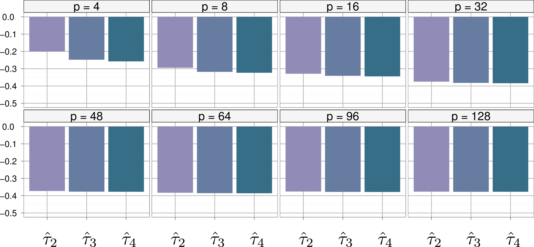
Recall that the “same order” scheme already provided a significant decrease in the variance of the estimation. In the light of our results, our interpretation is that using parallel chains with the same proposed values acts like a ”poor man” Rao–Blackwellization technique since times more uniforms are used. Specifically, each of the proposed values is proposed times instead of once, thus reducing the impact of each single uniform draw on the overall estimation.
When we use Rao–Blackwellization on top of the block IMH, in the estimators and , we try indeed to integrate out a randomness that already is partly gone. This explains why, although Rao–Blackwellization techniques provide a significant improvement over standard IMH, the improvement is much lower and thus rather unappealing when used in the block IMH setting. This outcome was at first frustrating since Rao–Blackwellization is indeed affordable at a cost of only . However, this shows in fine that the improvement brought by the block IMH algorithm roughly provides the same improvement as the Rao–Blackwell solution, at a much lower cost.
4.4 Comparison with Importance Sampling
The proposal density may also be used to construct directly an importance sampling (IS) estimator
where the values are drawn from . It therefore makes sense to compare the IMH algorithm with an IS approximation because IS is similarly easy to parallelize, and straightforward to program. Furthermore, since the IS estimator does not involve ancillary uniform variables, it is comparable to the Rao–Blackwellized version of IMH, and hence to the block IMH. Obviously, IS cannot necessarily be used in the settings when IMH algorithms are used, because the latter are also considered for approximating simulations from the target density . In particular, when considering Metropolis-within-Gibbs algorithms, IS cannot be used in a straightforward manner, even for approximating integrals.
Before giving numerical results for a comparison run on the toy example, we now explain why in this comparison we took the number of blocks to be larger than . The previous comparisons were computed with , i.e. on a single block and for a large number of independent runs. The choice of was then irrelevant since we were comparing methods that were exploiting in different ways the proposed values generated in each block. When considering the block IMH algorithm as a whole, as explained in Section 2, the end of each block sees a new starting value chosen from the current block. This ensures that the algorithm produces a valid Markov chain. However, our construction also implies that the successive blocks produced by the algorithm are correlated, which should lead to lesser performances than for the IS estimator.
In the comparison between IMH and IS, we therefore need to take into account this correlation between successive blocks. To this effect, we produce the variance reductions for several values of . Those reductions are presented in Figure 6 for and different values of . Once again, the permutations in the block IMH algorithm are chosen to be random.
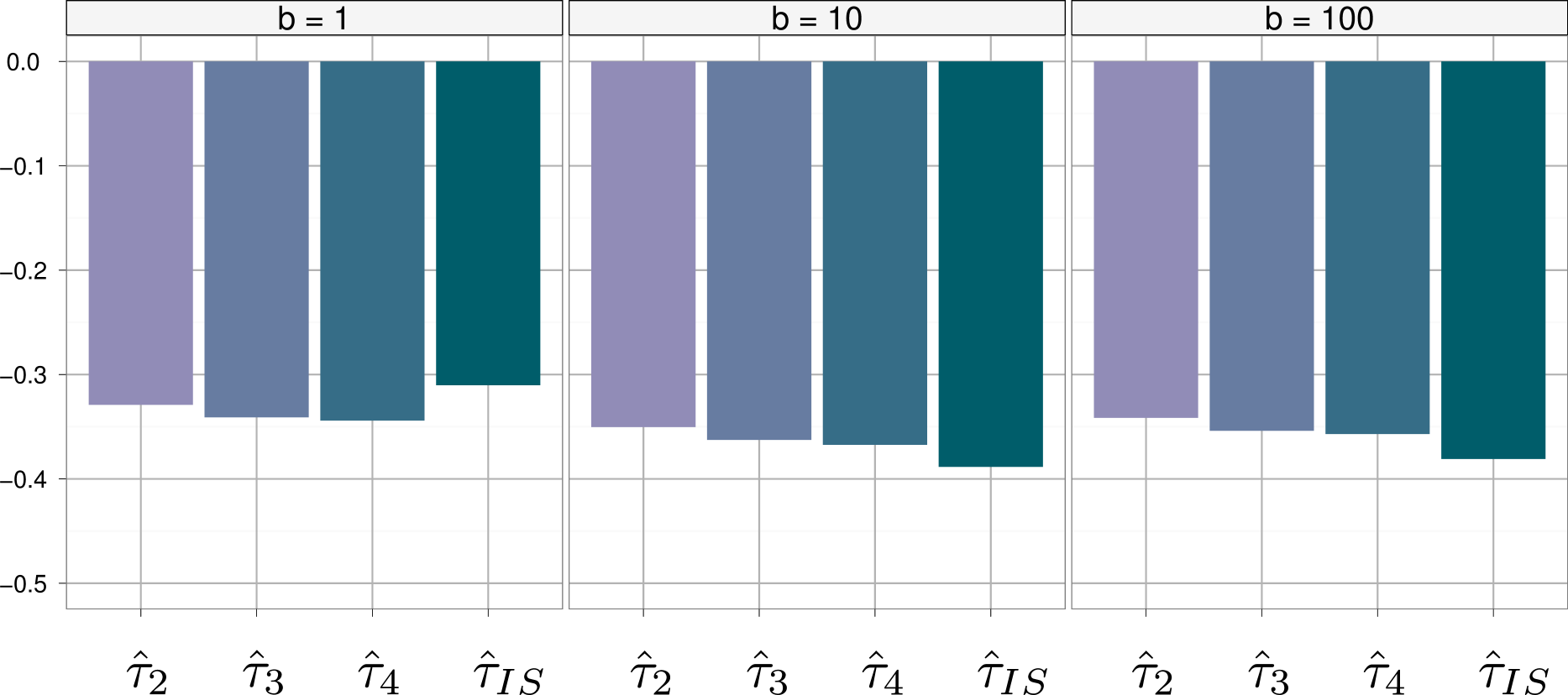
Figure 6 shows the a priori surprising result that, when selecting in the experiment, the variance results are in favor of the block IMH solutions over the IS estimator, but, for any realistic application, is (much) larger than . For all , the IS estimator has a smaller variance than the three alternative block IMH estimators, if only by a small margin. (Note that the variance improvement over the original MCMC estimator is slightly increasing with despite the correlation between blocks, given that the correlation between the terms involved in the block IMH estimators is lower than the correlation in the original MCMC chain.) This experiment thus shows that the block IMH solution gets very close to the IS estimator, while preserving the Markovian features of the original IMH algorithm.
5 A probit regression illustration
In order to evaluate the performances of the parallel processing presented in this paper on a realistic example, we examine its implementation for the probit model already analyzed in Marin and Robert (2010) for the comparison of model choice techniques because the “plug-in” normal distribution based on MLE estimates of the first two moments works perfectly as an independent proposal.
A probit model can be represented as a natural latent variable model in that, if we consider a sample of independent latent variables associated with a standard regression model, i.e. such that , where the ’s are -dimensional covariates and is the vector of regression coefficients, then such that
is a probit sample. Indeed, given , the ’s are independent Bernoulli rv’s with where is the standard normal cdf. The choice of a prior distribution for the probit model is open to debate, but the above connection with the latent regression model induced Marin and Robert (2007) to suggest a -prior model, , with as the factor and as the regressor matrix.
While a Gibbs sampler taking advantage of the latent variable structure is implemented in Marin and Robert (2010) and earlier references (Albert and Chib, 1993), a straightforward Metropolis–Hastings algorithm may be used as well, based on an independent proposal , where is the MLE estimator, its asymptotic variance, and a scaling factor.
As in Marin and Robert (2010) and Girolami and Calderhead (2010), we use the R Pima Indian benchmark dataset (R Development Core Team, 2006), which contains medical information about Pima Indian women with seven covariates and one explained binary diabetes variable.
For the purpose of illustrating the implementation of the block IMH algorithm, we only consider here three covariates, namely plasma glucose concentration (with coefficient ), diastolic blood pressure (with coefficient ) and diabetes pedigree function (with coefficient ). We are interested in the posterior mean of those three regression parameters. In our experiment, we ran independent replications of our algorithm to produce a reliable evaluation of the variance of the estimators under comparison. In Figure 7 we present the variance comparison of the four estimators described in Section 4, for and and for each of the three regression parameters. In the independent proposal, the scale factor is chosen to be since pilot runs showed that it led to an acceptance rate around , with thus enough rejections to exhibit improvement by Rao–Blackwellization.
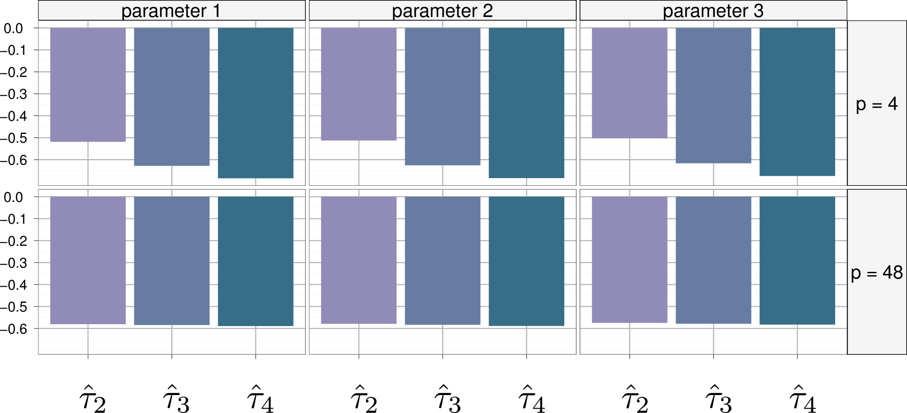
The results shown in Figure 7 confirm the huge decrease in variance previously observed in the toy example. The gains represented in those figures indicate that the block estimator is nearly as good (in terms of variance improvement) as the Rao–Blackwellized block estimators and , especially when moves from to . This confirms the previous interpretation given in Section 4 that the block IMH algorithm provides a cost-free Rao–Blackwellization as well as a partial averaging over the order of the proposed values.
The fact that the toy example showed decreases in the variance that were around whereas the probit regression shows decreases around is worth discussing. The amount of decrease in the variance differs from one example to the other, but it is more importantly depending on the acceptance rate of the Metropolis–Hastings algorithm. In fact, Rao–Blackwellization and permutations of the proposed values are useless steps if the acceptance rate is exactly . On the opposite, it may result in a significant improvement when the acceptance rate is low (since the part of the variance due to the uniform draws would then be much more important).
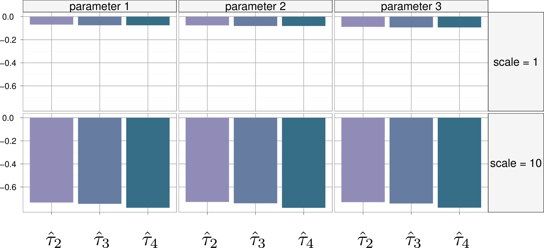
To illustrate the connection between the observed improvement and the acceptance rate, we propose in Figure 8 a variance comparison for and two scaling factors of the proposal covariance matrix in the probit regression model. In the previous experiment, we have used , which leads to an acceptance ratio around . Here, if we take , the acceptance ratio rises to , and hence almost all the proposed values are accepted. In this case permuting the proposed values and using Rao–Blackwellization techniques does not bring much of a variance decrease (Figure 8, top). On the other hand, if we take , the acceptance ratio drops down to and the observed decrease in variance is huge. In this second case using all the proposed values gives much better results than relying on the standard IMH estimator, which is only based on of the proposed values that were accepted (Figure 8, bottom).
The difference observed with this range of scaling factors is thus in agreement with the larger decrease in variance observed for the probit regression. This is a positive feature of the block IMH method, since in a complex model, the target distribution is most often poorly approximated by the proposal and thus the acceptance rate of the IMH algorithm is quite likely to be low.
6 Conclusion
The Monte Carlo experiments produced in this paper have shown that the proposed method improves significantly the precision of the estimation, when compared with the standard IMH algorithm. Beyond these examples, we see multiple situations where the block IMH algorithm can be used to improve the estimation in challenging problems. First, as already stated, the IMH algorithm can be used in Metropolis-within-Gibbs algorithms (Gilks et al., 1995). Obviously if a single IMH step is performed for each component of the state, then the block IMH technique cannot be applied without incurring additional costs. However, it is also correct to update each component multiple times instead of once. Furthermore, an uniform Gibbs scan is rarely the optimal way to update the components and more sophisticated schemes have been studied, resulting in random scan Gibbs samplers and adaptive Gibbs samplers (Latuszynski and Rosenthal, 2010), where the probability of updating a given component depends on the component and is learned along the iterations of the algorithm. Hence if a component is updated times more often than another, IMH can be performed in a row, which allows the use of the block IMH technique with .
IMH steps are also used within sequential Monte Carlo (SMC) samplers (Chopin, 2002, Del Moral and Doucet, 2003), to diversify the particles after resampling steps. In this context, an independent proposal can be designed by fitting a (usually Gaussian) distribution on the particles. If the move step is repeated multiple times in a row, for instance to ensure a satisfying particle diversification, then the block IMH algorithm can be used.
Related to SMC, another context where the variance reduction provided by block IMH might be valuable is the class of particle Markov Chain Monte Carlo methods (Andrieu et al., 2010). For these methods, a particle filter is computed at each iteration of the MH algorithm to estimate the target density, and hence it is paramount to make the most out of the expensive computations involved by those estimates. This is thus a natural framework for parallelization.
As a final message, the block IMH method is close to being parallel (except for the random draw of an index at the end of each block). Since parallel computing is getting increasingly easy to use, the free improvement brought by is available for all implementations of the IMH algorithm. Furthermore, even without considering parallel computing, since the method uses the most of each target density evaluation, it brings significant improvement when computing the target density is very costly. In such settings, the cost of drawing instead of uniform variates is negligible and the block IMH algorithm thus runs in about the same time as the standard IMH algorithm. We note that the time required to complete a block in the algorithm is essentially the maximum of the times required to calculate the density ratios . Therefore, if these times widely vary, there could be a diminishing saving in computation time as increases for both the standard IMH and the block IMH algorithms. Nonetheless, even in such extreme cases, using in the block IMH algorithm would bring a significant variance improvement at essentially no additional cost.
Acknowledgements
The work of the second author (CPR) was partly supported by the Agence Nationale de la Recherche (ANR, 212, rue de Bercy 75012 Paris) through the 2009 project ANR-08-BLAN-0218 Big’MC and the 2009 project ANR-09-BLAN-01 EMILE. Pierre Jacob is supported by a PhD fellowship from the AXA Research Fund. Since this research was initiated during the Valencia 9 Bayesian Statistics conference, the paper is dedicated to José Miguel Bernardo for the organization of this series of unique meetings since 1979. Discussions of the second author with participants during a seminar in Stanford University in August 2010 were quite helpful, in particular the suggestion made by Art Owen to include the “half-inversed half-random” permutations. The authors are grateful to Julien Cornebise for helpful discussions, in particular those leading to the stratified strategy, and to François Perron for his advice on the permutations. Comments and suggestions from the editorial team of JCGS were most helpful in improving the presentation of our results.
References
- Albert and Chib (1993) Albert, J. and Chib, S. (1993). Bayesian analysis of binary and polychotomous response data. J. American Statist. Assoc., 88 669–679.
- Andrieu et al. (2010) Andrieu, C., Doucet, A. and Holenstein, R. (2010). Particle Markov chain Monte Carlo (with discussion). J. Royal Statist. Society Series B, 72 357–385.
- Atchadé and Perron (2005) Atchadé, Y. and Perron, F. (2005). Improving on the independent Metropolis–Hastings algorithm. Statistica Sinica, 15 3–18.
- Casella and Robert (1996) Casella, G. and Robert, C. (1996). Rao-Blackwellisation of sampling schemes. Biometrika, 83 81–94.
- Chopin (2002) Chopin, N. (2002). A sequential particle filter method for static models. Biometrika, 89 539–552.
- Corander et al. (2006) Corander, J., Gyllenberg, M. and Koski, T. (2006). Bayesian model learning based on a parallel MCMC strategy. Statistics and Computing, 16 355–362.
- Craiu et al. (2009) Craiu, R., Rosenthal, J. and Yang, C. (2009). Learn from thy neighbour: Parallel-chain and regional adaptive MCMC. J. American Statist. Assoc., 104.
- Craiu and Meng (2005) Craiu, R. V. and Meng, X.-L. (2005). Multiprocess parallel antithetic coupling for backward and forward Markov chain Monte Carlo. Ann. Statist., 33 661–697.
- Del Moral and Doucet (2003) Del Moral, P. and Doucet, A. (2003). Sequential Monte Carlo samplers. Tech. rep., Dept. of Engineering, Cambridge Univ.
- Douc and Robert (2011) Douc, R. and Robert, C. (2011). A vanilla variance importance sampling via population Monte Carlo. Ann. Statist., 39 261–277.
- Gelfand and Smith (1990) Gelfand, A. and Smith, A. (1990). Sampling based approaches to calculating marginal densities. J. American Statist. Assoc., 85 398–409.
- Gilks et al. (1995) Gilks, W., Best, N. and Tan, K. (1995). Adaptive rejection Metropolis sampling within Gibbs sampling. Applied Statist. (Series C), 44 455–472.
- Girolami and Calderhead (2010) Girolami, M. and Calderhead, B. (2010). An object-oriented random-number package with many long streams and substreams. J. Royal Statist. Society Series B, 73 1–37.
- Hobert et al. (2002) Hobert, J., Jones, G., Presnel, B. and Rosenthal, J. (2002). On the applicability of regenerative simulation in Markov chain Monte Carlo. Biometrika, 89 731–743.
- Holmes et al. (2011) Holmes, C., Doucet, A., Lee, A., Giles, M. and Yau, C. (2011). Bayesian computation on graphics cards. In Bayesian Statistics 9: Proceedings of the Ninth Valencia International Meeting, June 3-8, 2010 (J. Bernardo, M. Bayarri, J. Degroot, A. Dawid, D. Heckerman, A. Smith and M. West, eds.). Oxford University Press.
- Latuszynski and Rosenthal (2010) Latuszynski, K. and Rosenthal, J. S. (2010). Adaptive Gibbs samplers. ArXiv e-prints. 1001.2797.
- L’Ecuyer et al. (2001) L’Ecuyer, P., Simard, R., Chen, E. J. and Kelton, W. D. (2001). An object-oriented random-number package with many long streams and substreams. Operations Research, 50 1073–1075.
- Lee et al. (2009) Lee, A., Yau, C., Giles, M., Doucet, A. and Holmes, C. (2009). On the utility of graphics cards to perform massively parallel simulation with advanced Monte Carlo methods. Arxiv preprint arXiv:0905.2441.
- Marin and Robert (2010) Marin, J. and Robert, C. (2010). Importance sampling methods for Bayesian discrimination between embedded models. In Frontiers of Statistical Decision Making and Bayesian Analysis (M.-H. Chen, D. Dey, P. Müller, D. Sun and K. Ye, eds.). Springer-Verlag, New York, 513–527.
- Marin and Robert (2007) Marin, J.-M. and Robert, C. (2007). Bayesian Core. Springer-Verlag, New York.
- Mykland et al. (1995) Mykland, P., Tierney, L. and Yu, B. (1995). Regeneration in Markov chain samplers. J. American Statist. Assoc., 90 233–241.
- Perron (1999) Perron, F. (1999). Beyond accept–reject sampling. Biometrika, 86 803–813.
- R Development Core Team (2006) R Development Core Team (2006). R: A Language and Environment for Statistical Computing. R Foundation for Statistical Computing, Vienna, Austria. URL http://www.R-project.org.
- Robert (1995) Robert, C. (1995). Convergence control techniques for MCMC algorithms. Statis. Science, 10 231–253.
- Robert and Casella (2004) Robert, C. and Casella, G. (2004). Monte Carlo Statistical Methods. 2nd ed. Springer-Verlag, New York.
- Rosenthal (2000) Rosenthal, J. (2000). Parallel computing and Monte Carlo algorithms. Far East J. Theoretical Statistics, 4 207–236.
- Suchard et al. (2010) Suchard, M., Wang, Q., Chan, C., Frelinger, J., Cron, A. and West, M. (2010). Understanding GPU programming for statistical computation: studies in massively parallel massive mixtures. Journal of Computational and Graphical Statistics, 19 418–438.
- Wraith et al. (2009) Wraith, D., Kilbinger, M., Benabed, K., Cappé, O., Cardoso, J.-F., Fort, G., Prunet, S. and Robert, C. (2009). Estimation of cosmological parameters using adaptive importance sampling. Physical Review D, 80 023507.