∎
2 University of Chinese Academy of Sciences, Beijing, China.
3 Centre for Artificial Intelligence and Robotics, Hong Kong Institute of Science & Innovation, Chinese Academy of Sciences, Hong Kong, China.
4 Shanghai Jiao Tong University, Shanghai, China.
5 Chinese University of Hong Kong, Hong Kong, China.
∗ Zhaoxiang Zhang is the corresponding author.
E-mail: {wanghaochen2022, zhaoxiang.zhang}@ia.ac.cn.
Using Unreliable Pseudo-Labels for Label-Efficient Semantic Segmentation
Abstract
The crux of label-efficient semantic segmentation is to produce high-quality pseudo-labels to leverage a large amount of unlabeled or weakly labeled data. A common practice is to select the highly confident predictions as the pseudo-ground-truths for each pixel, but it leads to a problem that most pixels may be left unused due to their unreliability. However, we argue that every pixel matters to the model training, even those unreliable and ambiguous pixels. Intuitively, an unreliable prediction may get confused among the top classes, however, it should be confident about the pixel not belonging to the remaining classes. Hence, such a pixel can be convincingly treated as a negative key to those most unlikely categories. Therefore, we develop an effective pipeline to make sufficient use of unlabeled data. Concretely, we separate reliable and unreliable pixels via the entropy of predictions, push each unreliable pixel to a category-wise queue that consists of negative keys, and manage to train the model with all candidate pixels. Considering the training evolution, we adaptively adjust the threshold for the reliable-unreliable partition. Experimental results on various benchmarks and training settings demonstrate the superiority of our approach over the state-of-the-art alternatives.
Keywords:
Semi-Supervised Learning Domain Adaption Weakly Supervised Learning Semantic Segmentation1 Introduction
Semantic segmentation is a fundamental task in the computer vision field and has been significantly advanced along with the rise of deep neural networks (Long et al., 2015a, ; Ronneberger et al., , 2015; Zhao et al., , 2017; Chen et al., 2017a, ). However, existing supervised approaches rely on large-scale annotated data, which can be too costly to acquire in practice. For instance, it takes around 90 minutes to annotate just a single image of Cityscapes (Cordts et al., , 2016), and this number even increases to 200 under adverse conditions (Sakaridis et al., , 2021). To alleviate this problem, many attempts have been made towards label-efficient semantic segmentation (Ru et al., , 2022; Wang et al., 2022b, ; Hoyer et al., , 2022). Under this setting, self-training, i.e., assigning pixel-level pseudo-labels for each weakly-labeled sample, becomes a typical solution. Specifically, given a weakly-labeled image, prior arts (Lee et al., , 2013; Xie et al., , 2020) borrow predictions from the model trained on labeled data or leverage Class Activation Maps (CAMs) (Zhou et al., , 2016) to obtain pixel-wise prediction, and then use them as the “ground-truth” to, in turn, boost the model. Along with it, many attempts have been made to produce high-quality pseudo-labels. A typical solution is to filter the predictions using their confidence scores (Yang et al., , 2022; Zou et al., , 2020; Zuo et al., , 2021; Xu et al., 2021b, ; Hoyer et al., , 2022; Ru et al., , 2022). In this way, only the highly confident predictions are served as the pseudo-labels, while those ambiguous ones are simply discarded.
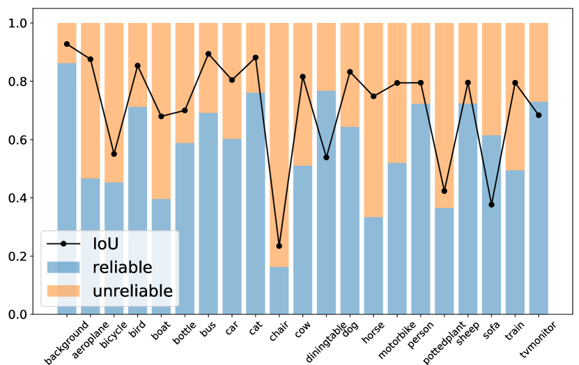
One potential problem caused by this paradigm is that some pixels may never be learned in the entire training process. For example, if the model cannot satisfyingly predict some certain class, it becomes difficult to assign accurate pseudo-labels to the pixels regarding such a class, which may lead to insufficient and categorically imbalanced training. For instance, as illustrated in Fig. 1, underperformed category chair tends to have fewer reliable predictions, and the model will be probably biased to dominant classes, e.g., background and cat, when we filter reliable predictions to be ground-truths for supervision and simply discard those ambiguous predictions. This issue even becomes more severe under domain adaptive or weakly supervised settings. Under both settings, predictions of unlabeled or weakly-labeled images usually run into undesirable chaos, and thus only a few pixels can be regarded as reliable ones when selecting highly confident pseudo-labels. From this perspective, we argue that to make full use of the unlabeled data, every pixel should be properly utilized.
However, how to use these unreliable pixels appropriately is non-trivial. Directly using the unreliable predictions as the pseudo-labels will cause the performance degradation (Arazo et al., , 2020) because it is almost impossible for unreliable predictions to assign exactly correct pseudo-labels. Therefore, in this paper, we propose an alternative way of Using Unreliable Pseudo-Labels (U2PL).
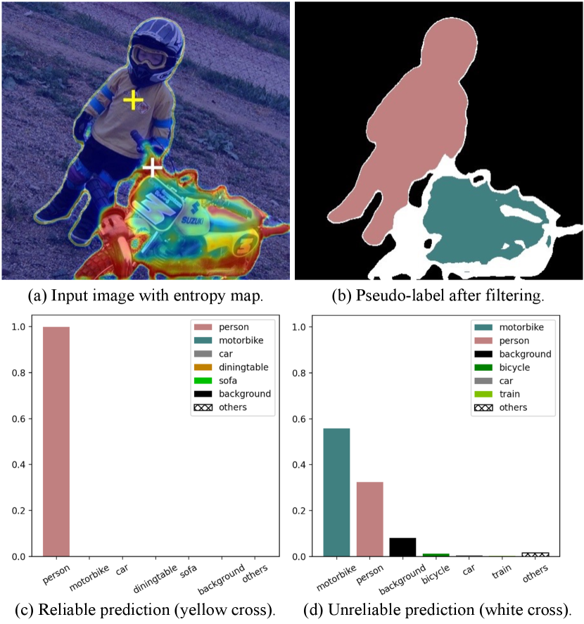
First, we observe that an unreliable prediction usually gets confused among only a few classes instead of all classes. Taking Fig. 2 as an instance, the pixel with a white cross is an unreliable prediction that receives similar probabilities on class motorbike and person, but the model is pretty sure about this pixel not belonging to class car and train. Based on this observation, we reconsider those unreliable pixels as the negative keys to those unlikely categories, which is a simple and intuitive way to make full use of all predictions. Specifically, after getting the prediction from an unlabeled image, we first leverage the per-pixel entropy as the metric (see Fig. 2a) to separate all pixels into two groups, i.e., reliable ones and unreliable ones. All reliable predictions are then used to derive positive pseudo-labels, while the pixels with unreliable predictions are pushed into a memory bank, which is full of negative keys. To avoid all negative pseudo-labels only coming from a subset of categories, we employ a queue for each category. Such a design ensures that the number of negative keys for each class is balanced, preventing being overwhelmed by those dominant categories. Meanwhile, considering that the quality of pseudo-labels becomes higher as the model gets more and more accurate, we come up with a strategy to adaptively adjust the threshold for the partition of reliable and unreliable pixels.
Extensions of the conference version (Wang et al., 2022b, ).
To better demonstrate the efficacy of using unreliable pseudo-labels, instead of studying only under the semi-supervised setting, we extend our original conference publication (Wang et al., 2022b, ) to domain adaptive and weakly-supervised settings, indicating that using unreliable pseudo-labels is crucial and effective on various label-efficient settings, bringing significant improvements consistently. Moreover, to produce high-quality pseudo-labels, we further make the category-wise prototype momentum updated during training to build a consistent set of keys and propose a denoising technique to enhance the quality of pseudo-labels. Additionally, a symmetric cross-entropy loss (Wang et al., , 2019) is used considering the pseudo-labels are still noisy even after filtering and denoising. We call the extended framework as UPL+.
In the following, we provide a brief discussion of how these three settings differ. Semi-supervised (SS) approaches aim to train a segmentation model with only a few labeled pixel-level ground-truths (Yang et al., , 2022; Chen et al., 2021c, ; Chen et al., 2021a, ; Alonso et al., , 2021; French et al., , 2020; Ouali et al., , 2020; Wang et al., 2022b, ) together with numerous unlabeled ones. Domain adaptive (DA) alternatives (Hoyer et al., , 2022; Zhang et al., 2021b, ; Li et al., 2022b, ; Hoffman et al., , 2018; Wang et al., 2020a, ; Wang et al., 2023b, ) introduce synthetic (source) datasets (Richter et al., , 2016; Ros et al., , 2016) into training and try to generalize the segmentation model to real-world (target) domains (Cordts et al., , 2016; Sakaridis et al., , 2021) without access to target labels. Because in most cases, dense labels for those synthetic datasets can be obtained with minor effort. Weakly-supervised (WS) methods (Ru et al., , 2022; Fan et al., 2020c, ; Fan et al., 2020b, ; Fan et al., 2020a, ; Li et al., 2022a, ; Zhang et al., 2020a, ) leverage weak supervision signals that are easier to obtain, such as image labels (Papandreou et al., , 2015), bounding boxes (Dai et al., , 2015), points (Fan et al., , 2022), scribbles (Lin et al., , 2016), instead of pixel-level dense annotations to train a segmentation model.
We evaluate the proposed UPL+ on both (1) SS, (2) DA, and (3) WS semantic segmentation settings, where UPL+ manages to bring significant improvements consistently over baselines. In SS, we evaluate our UPL+ on PASCAL VOC 2012 (Everingham et al., , 2010) and Cityscapes (Cordts et al., , 2016) under a wide range of training settings. In DA, we evaluate our UPL+ on two widely adopted benchmarks, i.e., GTA5 (Richter et al., , 2016) Cityscapes (Cordts et al., , 2016) and SYNTHIA (Ros et al., , 2016) Cityscapes (Cordts et al., , 2016). In WS, we evaluate our UPL+ on PASCAL VOC 2012 (Everingham et al., , 2010) benchmark using only image-level supervisions. Furthermore, through visualizing the segmentation results, we find that our method achieves much better performance on those ambiguous regions (e.g., the border between different objects), thanks to our adequate use of the unreliable pseudo-labels. Our contributions are summarized as follows:
-
1.
Based on the observation that unreliable predictions usually get confused among only a few classes instead of all classes, we build an intuitive framework U2PL that aims to mine the inherited information of discarded unreliable keys.
-
2.
We extend the original version of U2PL to (1) domain adaptive and (2) weakly supervised semantic segmentation settings, demonstrating that using unreliable pseudo-labels is crucial in both settings.
-
3.
To produce high-quality pseudo-labels, we further incorporate three carefully designed techniques, i.e., momentum prototype updating, prototypical denoising, and symmetric cross-entropy loss.
-
4.
UPL+ outperforms previous methods across extensive settings on both SS, DA, and WS benchmarks.
2 Related Work
Semantic segmentation aims to assign each pixel a pre-defined class label, and tremendous success in segmentation brought by deep convolutional neural networks (CNNs) has been witnessed (Ronneberger et al., , 2015; Long et al., 2015a, ; Yu and Koltun, , 2015; Chen et al., 2017a, ; Chen et al., 2017b, ; Zhao et al., , 2017; Chen et al., , 2018; Badrinarayanan et al., , 2017). Recently, Vision Transformers (ViTs) (Dosovitskiy et al., , 2021) provides a new feature extractor for images, and researchers have successfully demonstrated the feasibility of using ViTs in semantic segmentation (Zheng et al., , 2021; Xie et al., , 2021; Cheng et al., , 2021; Strudel et al., , 2021; Cheng et al., , 2022; Xu et al., , 2022). However, despite the success of these deep models, they usually thrive with dense per-pixel annotations, which are extremely expensive and laborious to obtain (Cordts et al., , 2016; Sakaridis et al., , 2021).
Semi-supervised semantic segmentation
methods aim to train a segmentation model with only a few labeled images and a large number of unlabeled images. There are two typical paradigms for semi-supervised learning: consistency regularization (Bachman et al., , 2014; Ouali et al., , 2020; French et al., , 2020; Sajjadi et al., , 2016; Xu et al., 2021b, ) and entropy minimization (Grandvalet and Bengio, , 2004; Chen et al., 2021a, ). Recently, a variant framework of entropy minimization, i.e., self-training (Lee et al., , 2013), has become the mainstream thanks to its simplicity and efficacy. On the basis of self-training, several methods (French et al., , 2020; Yuan et al., , 2021; Yang et al., , 2022; Wang et al., 2023e, ; Du et al., 2022b, ) further leverage strong data augmentation techniques such as (DeVries and Taylor, , 2017; Yun et al., , 2019; Olsson et al., , 2021), to produce meaningful supervision signals. However, in the typical weak-to-strong self-training paradigm (Sohn et al., , 2020), unreliable pixels are usually simply discarded. UPL+, on the contrary, fully utilizes those discarded unreliable pseudo-labels, contributing to boosted segmentation results.
Domain adaptive semantic segmentation
focuses on training a model on a labeled source (synthetic) domain and generalizing it to an unlabeled target (real-world) domain. This is a more complicated task compared with semi-supervised semantic segmentation due to the domain shift between source and target domains. To overcome the domain gap, most previous methods optimize some custom distance (Long et al., 2015b, ; Lee et al., 2019a, ; Wang et al., 2023b, ) or apply adversarial training (Goodfellow et al., , 2014; Nowozin et al., , 2016), in order to align distributions at the image level (Hoffman et al., , 2018; Murez et al., , 2018; Sankaranarayanan et al., , 2018; Li et al., , 2019; Gong et al., , 2019; Choi et al., , 2019; Wu et al., , 2019; Abramov et al., , 2020; Zhang et al., 2020b, ), intermediate feature level (Hoffman et al., , 2016; Hong et al., , 2018; Hoffman et al., , 2018; Saito et al., , 2018; Chang et al., , 2019; Chen et al., , 2019; Wan et al., , 2020; Li et al., 2021a, ; Wang et al., 2023b, ), or output level (Tsai et al., , 2018; Luo et al., , 2019; Melas-Kyriazi and Manrai, , 2021). Few studies pay attention to unreliable pseudo-labels under this setting. To the best of our knowledge, we are the first to recycle those unreliable predictions when there exists a distribution shift between different domains.
Weakly supervised semantic segmentation
seeks to train semantic segmentation models using only weak annotations, and can be mainly categorized into image-level labels (Du et al., 2022a, ; Ru et al., , 2022, 2023; Fan et al., 2020c, ; Fan et al., 2020a, ; Ahn and Kwak, , 2018; Lee et al., 2021c, ; Wu et al., , 2021; Li et al., 2021b, ; Lee et al., 2019b, ; Lee et al., 2021b, ), points (Fan et al., , 2022), scribbles (Lin et al., , 2016), and bounding boxes (Dai et al., , 2015). This paper mainly discusses the image-level supervision setting, which is the most challenging among all weakly supervised scenarios. Most methods (Wei et al., , 2017; Zhang et al., 2021a, ; Sun et al., , 2021; Jiang et al., , 2019; Kim et al., , 2021; Yao et al., , 2021) are designed with a multi-stage process, where a classification network is trained to produce the initial pseudo-masks at pixel level using CAMs (Zhou et al., , 2016). This paper focuses on end-to-end frameworks (Pinheiro and Collobert, , 2015; Papandreou et al., , 2015; Roy and Todorovic, , 2017; Zhang et al., 2020a, ; Araslanov and Roth, , 2020) in weakly supervised semantic segmentation with the goal of making full use of pixel-level predictions, i.e., CAMs.
Contrastive learning
is widely used by many successful works in unsupervised visual representation learning (Chen et al., , 2020; Chen et al., 2021b, ; Wang et al., 2023c, ; Wang et al., 2023a, ). In semantic segmentation, contrastive learning has become a promising new paradigm (Liu et al., , 2021; Wang et al., , 2021; Zhao et al., , 2021). The following methods try to go deeper by adopting the contrastive learning framework for semi-supervised semantic segmentation tasks. (Zhong et al., , 2021) minimizes the mean square error between two positive samples and introduces several strategies to sample negative pixels. (Alonso et al., , 2021) utilizes a class-wise memory bank to store representative negative pixels for each class. However, these methods ignore the common false negative samples in semi-supervised segmentation, where unreliable pixels may be wrongly pushed away in a contrastive loss. Based on the observation that unreliable predictions usually get confused among only a few categories, UPL+ alleviates this problem by discriminating the unlikely categories of unreliable pixels. In the field of domain adaptive semantic segmentation, only a few methods apply contrastive learning. (Kang et al., , 2020) adopts pixel-level cycle association in conducting positive pairs. (Zhou et al., , 2021) apply regional contrastive consistency regularization. (Wang et al., 2023b, ) introduces an image translation engine to ensure cross-domain positive pairs are matched precisely. The underlying motivation of these methods is to build a category-discriminative target representation space. However, we focus on how to make full use of unreliable pixels, which is quite different from existing contrastive learning-based DA alternatives. Contrastive learning is also studied in weakly supervised semantic segmentation. For instance, (Du et al., 2022a, ) proposes pixel-to-prototype contrast to improve the quality of CAMs by pulling pixels close to their positive prototypes. (Ru et al., , 2023) extend this idea by incorporating the self-attention map of ViTs. On the contrary, the goal of using contrastive learning in UPL+ is not to improve the quality of CAMs. The contrast of UPL+ is conducted after CAM values are obtained with the goal of fully using unreliable predictions.
Segment Anything Model
(SAM) (Kirillov et al., , 2023) shows strong generalization capabilities by training on over 1 billion object masks. However, it is important to note that SAM is not designed for semantic segmentation. Instead, it produces binary masks within an image. Given the impracticality of manually classifying each object mask from the SA-1B (Kirillov et al., , 2023) dataset into specific categories, label-efficient semantic segmentation is still worth studying. Moreover, only 1% masks of SA-1B are manually annotated. The authors have leveraged a segmentation model to assist in data collection and enhance mask diversity. They even include a fully automated annotation phase, where the model generates masks without any human input, accounting for 99.1% of the masks. Based on this, we hypothesize that an appropriate self-training pipeline might contribute to a more powerful segmentation model. It is also worth noting that SAM is not universally effective across all domains. For instance, it fails in medical segmentation and camouflaged object segmentation (Ji et al., , 2023). To adapt SAMs to specific domains, additional domain-specific annotations are typically required. Specifically, Ma et al., (2024) combined a large amount of public-available medical segmentation datasets and built a dataset with over 1.5M image-mask pairs, which is much less diverse compared with the SA-1B dataset due to the absence of unlabeled images. We believe that developing an efficient pipeline for adapting SAM to specific domains, leveraging unlabeled data with minimal annotation costs, is also a worthwhile direction for future research.
3 Method
In this section, we first introduce background knowledge of label-efficient semantic segmentation in Sec. 3.1. Next, the elaboration of UPL+ is described in Sec. 3.2. In Sec. 3.3 and Sec. 3.4, we introduce how to filter high-quality pseudo-labels and the denoising technique, respectively. Then, in Sec. 3.5, we specify how UPL+ can be used in three label-efficient learning tasks, i.e., semi-supervised/domain adaptive, and weakly supervised settings.
3.1 Preliminaries
Label-efficient semantic segmentation. The common goal of label-efficient semantic segmentation methods is leveraging the incomplete set of labels to train a model that segments well on the whole set of images , where indicates the total images and is the number of labeled samples. where and are input resolutions. The first image samples are matched with unique labels, and they consist of the labeled set , while the remaining samples consist of the unlabeled set .
In practice, usually, we have and each label is the one-hot pixel-level annotation, where is the number of categories. The labeled set is collected from distribution while the unlabeled set is sampled from distribution . A general case is , and thus the problem falls into domain adaptive semantic segmentation. Otherwise, if , it is usually treated as a semi-supervised semantic segmentation task.
However, when but those labels are not collected at pixel-level, it becomes weakly supervised semantic segmentation. Under such a setting, each image is matched with its corresponding weak label , such as image labels (Papandreou et al., , 2015), bounding boxes (Dai et al., , 2015), points (Fan et al., , 2022), and scribbles (Lin et al., , 2016), and thus . This paper studies the image-level supervision setting, i.e., , which is the most challenging scenario. Note that is not the one-hot label since each image usually contains more than one category.
The overall objective of both settings usually contains a supervised term and an unsupervised term :
| (1) |
where is the weight of the unsupervised loss, which controls the balance of these two terms. Next, we will introduce the conventional pipeline of different settings, respectively.
Semi-supervised and domain adaptive semantic segmentation.
The typical paradigm of these two settings is the self-training framework (Tarvainen and Valpola, , 2017; Sohn et al., , 2020), which consists of two models with the same architecture, named teacher and student, respectively. These two models differ only when updating their weights. indicates the weight of the student and is updated consistently with the common practice using back-propagation, while the teacher’s weights are exponential moving average (EMA) updated by the student’s weights:
| (2) |
where is the momentum coefficient.
Each model consists of an encoder , a segmentation head , and a representation head used only for UPL+. At each training step, we equally sample labeled images and unlabeled images , and try to minimize Eq. (1). Mathematically, is the vanilla pixel-level cross-entropy:
| (3) | ||||
where indicates the -th labeled image and represents the corresponding one-hot hand-annotated segmentation map. is the composition function of and , which means the images are first fed into and then to get segmentation results. As the unsupervised term , we set it as the symmetric cross-entropy (SCE) loss (Wang et al., , 2019) for a stable training procedure, especially in the early stage. When computing , we first take each unlabeled sample into the teacher model and get predictions. Then, based on the pixel-level entropy map, we ignore unreliable pseudo-labels. Specifically,
| (4) | ||||
where is the one-hot pseudo-label for the -th unlabeled image. We set to and to follow (Wang et al., , 2019) and (Zhang et al., 2021b, ).
By minimizing and simultaneously, the model is able to leverage both the small labeled set and the larger unlabeled set .
Weakly supervised semantic segmentation using image-level labels.
Weakly supervised semantic segmentation methods aim to leverage CAMs (Zhou et al., , 2016) to produce pixel-level pseudo-masks first and then train a segmentation module synchronously (Ru et al., , 2022; Araslanov and Roth, , 2020), i.e., end-to-end, or asynchronously (Du et al., 2022a, ; Lee et al., 2021c, ), i.e., multi-stage. We begin with a brief review of how to generate CAMs.
Given an image classifier, e.g., ResNet (He et al., , 2016) and ViT (Dosovitskiy et al., , 2021), we denote the last feature maps as , where is the spatial size and indicates the channel dimension. The activation map for class is generated via weighting the feature maps with their contribution to class :
| (5) |
where is the parameters of the last fully connected layers. Then, min-max normalization is applied to re-scale to . is used to discriminate foreground regions from background, i.e., when the value of of a particular pixel is larger then , it is regarded as reliable predictions as well as pseudo-labels.
At each training step, we randomly sample images and their corresponding image-level labels, resulting in a batch . Since we only have image-level labels this time, an additional MLP is introduced to perform image-level classification, and the supervised loss is thus the multi-label soft margin loss:
| (6) |
As for the unsupervised term , it is the vanilla cross-entropy loss that leverages to be supervision signals:
| (7) |
where the pixel-level pseudo-label is generated by a simple threshold strategy following (Ru et al., , 2022):
| (8) |
where is the indicator function.
3.2 Elaboration of UPL+
In label-efficient learning, discarding unreliable pseudo-labels is widely used to prevent performance degradation (Zou et al., , 2020; Yang et al., , 2022; Sohn et al., , 2020; Xie et al., , 2020). However, such contempt for unreliable pseudo-labels may result in information loss. It is obvious that unreliable pseudo-labels can provide information for better discrimination. For example, the white cross in Fig. 2, is typically an unreliable pixel, whose distribution demonstrates its uncertainty to distinguish between class person and class motorbike. However, this distribution also demonstrates its certainty not to discriminate this pixel as class car, class train, class bicycle, and so on. Such characteristic gives us the main insight of using unreliable pseudo-labels for label-efficient semantic segmentation.
Mathematically, UPL+ aims to recycle unreliable predictions into training by adding an extra term into Eq. (1). Therefore, the overall objective becomes to
| (9) |
where is an extra weight to balance its contribution. Specifically, is the pixel-level InfoNCE (Oord et al., , 2018) loss:
| (10) | ||||
where is the total number of anchor pixels, and denotes the representation of the -th anchor of class . Each anchor pixel is followed with a positive key and negative keys, whose representations are and , respectively. is the output of the representation head. is the cosine similarity between features from two different pixels, whose range is limited between to , hence the need for temperature . We set , and in practice. How to select (a) anchor pixels (queries) , (b) the positive key for each anchor, and (c) negative keys for each anchor, is different among different label-efficient settings.
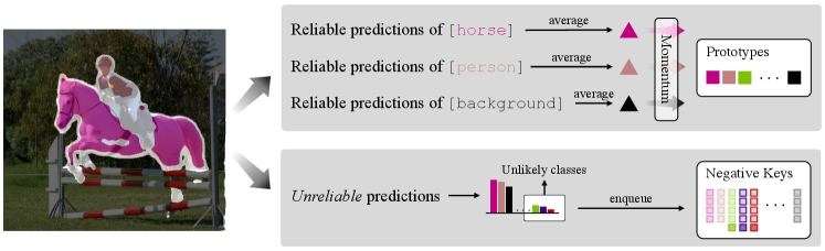
Fig. 3 illustrates how UPL+ conducts contrastive pairs. Concretely, predictions are first split into reliable ones and unreliable ones by leveraging the pixel-level entropy map. Reliable predictions (pixels marked in color other than white) are first averaged and then used to update category-wise prototypes, which are served as positive keys for given queries. Unreliable predictions (pixels marked in white) are served as negative keys regarding unlikely classes and are pushed into category-wise memory banks.
Next, we introduce how to apply UPL+ to label-efficient semantic segmentation as follows. Specifically, we first introduce how we produce pseudo-labels in Sec. 3.3. Next, denoising techniques are described in Sec. 3.4. Finally, how to sample contrastive pairs are explored in Sec. 3.5. Note that pseudo-labeling and denoising is used only in semi-supervised and domain-adaptive semantic segmentation.
3.3 Pseudo-Labeling
To avoid overfitting incorrect pseudo-labels, we utilize entropy of every pixel’s probability distribution to filter high-quality pseudo-labels for further supervision. Specifically, we denote as the softmax probabilities generated by the segmentation head of the teacher model for the -th unlabeled image at pixel , where is the number of classes. Its entropy is computed by:
| (11) |
where is the value of at -th dimension.
Then, we define pixels whose entropy on top as unreliable pseudo-labels at training epoch . Such unreliable pseudo-labels are not qualified for supervision. Therefore, we define the pseudo-label for the -th unlabeled image at pixel as:
| (12) |
where represents the entropy threshold at -th training step. We set as the quantile corresponding to , i.e., = np.percentile(H.flatten(),100*(1-)), where H is per-pixel entropy map. We adopt the following adjustment strategies in the pseudo-labeling process for better performance.
Dynamic Partition Adjustment.
During the training procedure, the pseudo-labels tend to be reliable gradually. Base on this intuition, we adjust unreliable pixels’ proportion with linear strategy every epoch:
| (13) |
where is the initial proportion and is set to , and is the current training epoch.
Adaptive Weight Adjustment.
After obtaining reliable pseudo-labels, we involve them in the unsupervised loss in Eq. (LABEL:eq:unsloss). The weight for this loss is defined as the reciprocal of the percentage of pixels with entropy smaller than threshold in the current mini-batch multiplied by a base weight :
| (14) |
where is the indicator function and is set to .
3.4 Pseudo-Label Denoising
It is widely known that self-training-based methods often suffer a lot from confirmation bias (Arazo et al., , 2020). Filtering reliable pseudo-labels (Yang et al., , 2022; Zou et al., , 2020) (which has been introduced in Sec. 3.3) and applying strong data augmentation (Yun et al., , 2019; DeVries and Taylor, , 2017; Olsson et al., , 2021) are two typical ways to face this issue. However, considering the domain shift between the labeled source domain and the unlabeled target domain, the model tends to be over-confident (Zhang et al., 2021b, ) and there is not enough to simply select pseudo-labels based on their reliability. To this end, we maintain a prototype for each class and use them to denoise those pseudo-labels.
Let be the prototype of class , as known as the center of the representation space
| (15) |
and concretely, contains all labeled pixels belongs to class and reliable unlabeled pixels predicted to probably belongs to class :
| (16) |
where and denote the representation space of labeled pixels and unlabeled pixels respectively:
| (17) | ||||
where index means the -th labeled (unlabeled) image, and index means the -th pixel of that image.
Momentum Prototype.
For the stability of training, all representations are supposed to be consistent (He et al., , 2020), forwarded by the teacher model hence, and are momentum updated by the centroid in the current mini-batch. Specifically, for each training step, the prototype of class is estimated as
| (18) |
where is the current center defined by Eq. (15) and is the prototype for last training step, and is the momentum coefficient which is set to .
Prototypical Denoising.
Let be the weight between -th unlabeled image and each class. Concretely, we define as the softmax over feature distances to prototypes:
| (19) |
Then, we get denoised prediction vector for pixel of -th unlabeled image based on its original prediction vector and class weight :
| (20) |
where denotes the element-wise dot.
Finally, we take into Eq. (12) and get denoised pseudo-label for pixel of the -th unlabeled image in Eq. (LABEL:eq:unsloss).
3.5 Contrastive Pairs Sampling
Formulated in Eq. (10), our UPL+ aims to make sufficient use of unreliable predictions by leveraging an extra contrastive objective that pulls positive pairs together while pushes negatives pairs away. In the following, we provide a detailed description on conducting contrastive pairs for both settings.
3.5.1 For SS and DA Settings
Anchor Pixels (Queries). During training, we sample anchor pixels (queries) for each class that appears in the current mini-batch. We denote the set of features of all labeled candidate anchor pixels for class as ,
| (21) |
where is the ground truth for the -th pixel of labeled image , and denotes the positive threshold for a particular class and is set to following (Liu et al., , 2021). means the representation of the -th pixel of labeled image . For unlabeled data, counterpart can be computed as:
| (22) |
It is similar to , and the only difference is that we use pseudo-label based on Eq. (12) rather than the hand-annotated label, which implies that qualified anchor pixels are reliable, i.e., . Therefore, for class , the set of all qualified anchors is
| (23) |
Positive Keys.
The positive sample is the same for all anchors from the same class. It is the prototype of class defined in Eq. (15):
| (24) |
Negative Keys.
We define a binary variable to identify whether the -th pixel of image is qualified to be negative samples of class .
| (25) |
where and are indicators of whether the -th pixel of labeled and unlabeled image is qualified to be negative samples of class respectively.
For -th labeled image, a qualified negative sample for class should be: (a) not belonging to class ; (b) difficult to distinguish between class and its ground-truth category. Therefore, we introduce the pixel-level category order . Obviously, we have and .
| (26) |
where is the low-rank threshold. Here, a small represents an aggressive strategy, which tries to make full use of unreliable predictions but may introduce too much noise. We set to it . Two indicators reflect (a) and (b), respectively.
For -th unlabeled image, a qualified negative sample for class should: (a) be unreliable; (b) probably not belongs to class ; (c) not belongs to most unlikely classes. Similarly, we also use to define :
| (27) |
where is the high-rank threshold and is set to . Finally, the set of negative samples of class is
| (28) |
Category-wise Memory Bank.
Due to the long tail phenomenon of the dataset, negative candidates in some particular categories are extremely limited in a mini-batch. In order to maintain a stable number of negative samples, we use category-wise memory bank (FIFO queue) to store the negative samples for class . We simply follow MoCo (He et al., , 2020), setting the queue size to . A large queue size contributes diverse negative samples while introducing extra computational costs.
Finally, the whole process to use unreliable pseudo-labels is shown in Algorithm 1. All features of anchors are attached to the gradient, and come from the student hence, while features of positive and negative samples are from the teacher.
3.5.2 For the WS Setting
The main difference when applying UPL+ to the WS setting is we do not have any pixel-level annotations now, and thus Eqs. (21) and (26) are invalid. Also, pseudo-labeling and denoising techniques introduced in Secs. 3.3 and 3.4 are not necessary here. This is because applying a simple threshold to re-scaled CAMs to discriminate foreground regions from the background is effective (Ru et al., , 2022). To this end, the elaboration of UPL+ on weakly supervised semantic segmentation becomes much easier. Next, how to select (1) anchor pixels, (2) positive keys, and (3) negative keys, are described in detail.
Anchor Pixels (Queries).
This time, as segmentation maps of the whole dataset are inaccessible, we cannot sample anchors using ground-truth labels as Eq. (21) does. Instead, we simply regard those pixels with a value of CAM larger than as candidates:
| (29) |
Positive Keys.
Similarly, positive keys for each query are the prototype of class , i.e., . Similarly, the prototypes are momentum updated described in Eq. (18), but category-wise centroids of the current mini-batch are computed by
| (30) |
Negative Keys.
Determining negative keys is much easier under the weakly supervised setting because a set of image-level labels is given for each image. Concretely, given a image , its image-level label is , where indicates that class exists in this image and vise versa. Therefore, the indicator representing whether pixel from the -th image is a qualified negative key for class natually becomes
| (31) |
where the first term means this image does not contain category at all, while the second term indicates this prediction is unreliable to determine the pixel belongs to category . The prediction becomes a qualified negative key when either of these two conditions is met.
4 Experiments
We conduct experiments on (1) semi-supervised, (2) domain adaptive, and (3) weakly supervised semantic segmentation benchmarks to verify the effectiveness of UPL+. The settings, baselines, and quantitative and qualitative results are provided in Secs. 4.1, 4.2, and 4.3. Due to limited computational resources, ablation studies are conducted only on semi-supervised benchmarks.
| Method | 1/16 (92) | 1/8 (183) | 1/4 (366) | 1/2 (732) | Full (1464) |
| SupOnly | 45.77 | 54.92 | 65.88 | 71.69 | 72.50 |
| MT† | 51.72 | 58.93 | 63.86 | 69.51 | 70.96 |
| CutMix† | 52.16 | 63.47 | 69.46 | 73.73 | 76.54 |
| PseudoSeg | 57.60 | 65.50 | 69.14 | 72.41 | 73.23 |
| PC2Seg | 57.00 | 66.28 | 69.78 | 73.05 | 74.15 |
| UPL | 67.98 | 69.15 | 73.66 | 76.16 | 79.49 |
| UPL+ | 69.29 | 73.40 | 75.03 | 77.09 | 79.52 |
4.1 Experiments on Semi-Supervised Segmentation
In this section, we provide experimental results on semi-supervised semantic segmentation benchmarks. We first describe the experimental setup, including datasets, network structure, evaluation metric, and implementation details. Then, we compare with recent methods in Sec. 4.1.1, and perform ablation studies on both PASCAL VOC 2012 and Cityscapes in Sec. 4.1.2. Moreover, in Sec. 4.1.3, we provide qualitative segmentation results.
| Method | Blender PASCAL VOC 2012 | Method | Cityscapes | |||||||
| 1/16 (662) | 1/8 (1323) | 1/4 (2646) | 1/2 (5291) | 1/16 (186) | 1/8 (372) | 1/4 (744) | 1/2 (1488) | |||
| SupOnly | 67.87 | 71.55 | 75.80 | 77.13 | SupOnly | 65.74 | 72.53 | 74.43 | 77.83 | |
| MT† | 70.51 | 71.53 | 73.02 | 76.58 | MT† | 69.03 | 72.06 | 74.20 | 78.15 | |
| CutMix† | 71.66 | 75.51 | 77.33 | 78.21 | CutMix† | 67.06 | 71.83 | 76.36 | 78.25 | |
| CCT | 71.86 | 73.68 | 76.51 | 77.40 | CCT | 69.32 | 74.12 | 75.99 | 78.10 | |
| GCT | 70.90 | 73.29 | 76.66 | 77.98 | GCT | 66.75 | 72.66 | 76.11 | 78.34 | |
| CPS | 74.48 | 76.44 | 77.68 | 78.64 | CPS† | 69.78 | 74.31 | 74.58 | 76.81 | |
| AEL | 77.20 | 77.57 | 78.06 | 80.29 | AEL† | 74.45 | 75.55 | 77.48 | 79.01 | |
| UPL | 77.21 | 79.01 | 79.30 | 80.50 | UPL | 74.90 | 76.48 | 78.51 | 79.12 | |
| UPL+ | 77.23 | 79.35 | 80.21 | 80.78 | UPL+ | 76.09 | 78.00 | 79.02 | 79.62 | |
Datasets.
In semi-supervised semantic segmentation, PASCAL VOC 2012 (Everingham et al., , 2010) and Cityscapes (Cordts et al., , 2016) are two widely used datasets for evaluation. PASCAL VOC 2012 Dataset is a standard semantic segmentation benchmark with 20 semantic classes of objects and 1 class of background. The training set and the validation set include and images respectively. Following (Hu et al., , 2021; Yang et al., , 2022; Chen et al., 2021c, ), we use SBD (Hariharan et al., , 2011) as the augmented set with additional training images. Since the SBD dataset is coarsely annotated, (Zou et al., , 2020) takes only the standard images as the whole labeled set, while other methods (Chen et al., 2021c, ; Hu et al., , 2021) take all images as candidate labeled data. Therefore, we evaluate our method on both the classic set ( candidate labeled images) and the blender set ( candidate labeled images). Cityscapes, a dataset designed for urban scene understanding, consists of training images with fine-annotated masks and validation images. For each dataset, we compare UPL+ with other methods under , , , and partition protocols.
Network Structure.
For SS segmentation, we use ResNet-101 (He et al., , 2016) pre-trained on ImageNet-1K (Deng et al., , 2009) as the backbone and DeepLabv3+ (Chen et al., , 2018) as the decoder. The representation head consists of two Conv-BN-ReLU blocks, where both blocks preserve the feature map resolution, and the first block halves the number of channels, mapping the extracted features into dimensional representation space. The architecture of the representation head remains the same in three different settings. The extra representation head introduces an additional 2.8 M parameters, resulting in roughly 10% more computational overhead compared to the baseline.
Evaluation Metric.
We adopt the mean of Intersection over Union (mIoU) as the metric to evaluate these cropped images. For the SS segmentation task, all results are measured on the val set on both Cityscapes (Cordts et al., , 2016) and PASCAL VOC 2012 (Everingham et al., , 2010), where VOC images are center cropped to a fixed resolution while slide window evaluation is used for Cityscapes following common practices (Hu et al., , 2021; Wang et al., 2022b, ).
Implementation Details.
For the training on the blender and classic PASCAL VOC 2012 dataset, we use stochastic gradient descent (SGD) optimizer with initial learning rate , weight decay as , crop size as , batch size as and training epochs as . For the training on the Cityscapes dataset, we also use stochastic gradient descent (SGD) optimizer with an initial learning rate of , weight decay as , crop size as , batch size as and training epochs as . In all experiments, the decoder’s learning rate is ten times that of the backbone. We use the poly scheduling to decay the learning rate during the training process: . All SS experiments are conducted with Tesla V100 GPUs.
| Blender VOC | Cityscapes | |||||
| R | U | 1/8 (1323) | 1/4 (2646) | 1/4 (744) | 1/2 (1488) | |
| ✓ | 74.29 | 75.76 | 74.39 | 78.10 | ||
| ✓ | 75.15 | 76.48 | 74.60 | 77.93 | ||
| ✓ | 78.37 | 79.01 | 77.19 | 78.16 | ||
| ✓ | ✓ | 77.30 | 77.35 | 75.16 | 77.19 | |
| ✓ | ✓ | 79.35 | 80.21 | 79.02 | 79.62 | |
| ✓ | ✓ | ✓ | 77.40 | 77.57 | 74.51 | 76.96 |
4.1.1 Comparison with State-of-the-Art Alternatives
We compare our method with following recent representative semi-supervised semantic segmentation methods: Mean Teacher (MT) (Tarvainen and Valpola, , 2017), CCT (Ouali et al., , 2020), GCT (Ke et al., , 2020), PseudoSeg (Zou et al., , 2020), CutMix (French et al., , 2020), CPS (Chen et al., 2021c, ), PC2Seg (Zhong et al., , 2021), AEL (Hu et al., , 2021). We re-implement MT (Tarvainen and Valpola, , 2017), CutMix (Yun et al., , 2019) for a fair comparison. For Cityscapes (Cordts et al., , 2016), we also reproduce CPS (Chen et al., 2021c, ) and AEL (Hu et al., , 2021). All results are equipped with the same network architecture (DeepLabv3+ as decoder and ResNet-101 as encoder). It is important to note the classic PASCAL VOC 2012 Dataset and blender PASCAL VOC 2012 Dataset only differ in the training set. Their validation set is the same with images.
Results on classic PASCAL VOC 2012 Dataset.
Tab. 1 compares our method with the other state-of-the-art methods on classic PASCAL VOC 2012 Dataset. UPL+ outperforms the supervised baseline by , , , , and under , , , , and “full” partition protocols respectively, indicating that semi-supervised learning fully mines the inherent information of unlabeled images. When comparing to state-of-the-arts, our UPL+ outperforms PC2Seg under all partition protocols by , , , , and respectively. Note that when labeled data is extremely limited, e.g., when we only have labeled data, our UPL+ outperforms previous methods by a large margin ( under split for classic PASCAL VOC 2012), proofing the efficiency of using unreliable pseudo-labels. Furthermore, by introducing extra strategies, UPL+ can outperform its previous version UPL by , , , , and respectively. The fewer labeled images we have, the larger improvement it brings, indicating that UPL+ is more capable of dealing with training noise than UPL.
Results on blender PASCAL VOC 2012 Dataset.
Tab. 2 shows the comparison results on blender PASCAL VOC 2012 Dataset. Our method UPL+ outperforms all the other methods under various partition protocols. Compared with the supervised baseline, UPL+ achieves improvements of , , and under , , and partition protocols respectively. Compared with the existing state-of-the-art methods, UPL+ surpasses them under all partition protocols. Especially under protocol and protocol, UPL+ outperforms AEL by and . When comparing UPL+ to its previous version UPL, it brings improvements of , , , and respectively. Compared to the classic VOC counterpart, it seems that UPL+ may struggle to bring significant improvements when we access adequate labeled images (i.e., the number of labeled data is extended from to ).
| PD | MP | SCE | DPA | PRT | Un | 1/4 (2646) | ||
| 77.33 | ||||||||
| ✓ | 77.08 | |||||||
| ✓ | ✓ | ✓ | ✓ | 78.49 | ||||
| ✓ | ✓ | ✓ | ✓ | 79.07 | ||||
| ✓ | ✓ | ✓ | ✓ | 77.57 | ||||
| ✓ | ✓ | ✓ | ✓ | ✓ | 79.30 | |||
| ✓ | 77.93 | |||||||
| ✓ | 77.69 | |||||||
| ✓ | ✓ | 78.01 | ||||||
| ✓ | ✓ | ✓ | 78.24 | |||||
| ✓ | ✓ | ✓ | ✓ | ✓ | ✓ | ✓ | ✓ | 80.21 |
| 1/16 (662) | 1/8 (1323) | 1/4 (2646) | 1/2 (5291) | |
| UPL+ (w/o PD) | 77.09 | 79.10 | 79.48 | 80.43 |
| UPL+ (w/ PD) | 77.23 | 79.35 | 80.21 | 80.78 |
| Blender VOC | Cityscapes | |||
| 1/8 (1323) | 1/4 (2646) | 1/4 (744) | 1/2 (1488) | |
| 0.9 | 79.07 | 79.29 | 77.81 | 78.51 |
| 0.99 | 78.91 | 79.37 | 77.93 | 78.54 |
| 0.999 | 79.35 | 80.21 | 79.02 | 79.62 |
| 0.9999 | 79.18 | 79.91 | 78.82 | 79.11 |
| Blender VOC | Cityscapes | ||||
| 1/8 (1323) | 1/4 (2646) | 1/8 (372) | 1/4 (744) | ||
| 0 | 1 | 77.76 | 78.63 | 76.71 | 78.02 |
| 1 | 0 | 79.06 | 79.68 | 77.03 | 78.53 |
| 0.1 | 1 | 79.11 | 79.83 | 77.43 | 78.72 |
| 1 | 0.5 | 79.35 | 80.21 | 78.00 | 79.02 |
| 0.5 | 0.5 | 79.33 | 80.20 | 77.79 | 78.81 |
Results on Cityscapes Dataset.
Tab. 2 illustrates the comparison results on the Cityscapes val set. UPL+ improves the supervised only baseline by , , and under , , , and partition protocols, and outperforms existing state-of-the-art methods by a notable margin. In particular, UPL+ outperforms AEL by , , and under , , , and partition protocols Compared to its previous version UPL, UPL+ achieves improvements of , , , and respectively.
4.1.2 Ablation Studies
In this section, we first design experiments in Tab. 3 to validate our main insight: using unreliable pseudo-labels is significant for semi-supervised semantic segmentation. Next, we ablate each component of our proposed UPL+ in Tab. 4, including using contrastive learning (), applying a memory bank to store abundant negative samples (), prototype-based pseudo-labels denoising (PD), momentum prototype (MP), using symmetric cross-entropy for unlabeled images (SCE), dynamic partition adjustment (DPA), probability rank threshold (PRT), and only regard unreliable pseudo-labels as negative samples (Un). In Tab. 5, we evaluate the performance of prototypical denoising under different partition protocols on both PASCAL VOC 2012 and Cityscapes. Finally, we ablate the hyper-parameter for momentum prototype, for symmetric cross-entropy loss, for probability rank threshold, initial reliable-unreliable partition , base learning rate , and temperature , respectively.
Effectiveness of Using Unreliable Pseudo-Labels.
To prove our core insight, i.e., using unreliable pseudo-labels promotes semi-supervised semantic segmentation, we conduct experiments about selecting negative candidates (which is described in Sec. 3.5) with different reliability, i.e., whether to regard only unreliable pseudo-labels to be negative samples of a particular query.
Tab. 3 demonstrates the mIoU results on PASCAL VOC 2012 val set and Cityscapes val set, respectively. Containing “U” in negative keys outperforms other options, proving using unreliable pseudo-labels does help, and our UPL+ fully mines the information of all pixels, especially those unreliable ones. Note that “R” in Tab. 3 indicates negative keys in memory banks are reliable. Containing both “U” and “R” means that all features are stored in memory banks without filtering. It is worth noticing that containing features from labeled set brings marginal improvements, but significant improvements are brought because of the introduction of unreliable predictions, i.e., “U” in Tab. 3.
Effectiveness of Components.
We conduct experiments in Tab. 4 to ablate each component of UPL+ step by step. For a fair comparison, all the ablations are under 1/4 partition protocol on the blender PASCAL VOC 2012 Dataset.
Above all, we use no trained model as our baseline, achieving mIoU of (CutMix in Tab. 2). We first ablate components in contrastive learning, including , DPA, PRT, and Un. Simply adding vanilla even contributes to the performance degradation by . Category-wise memory bank , along with PRT and high entropy filtering brings an improvement by to vanilla . Dynamic Partition Adjustment (DPA) together with high entropy filtering, brings an improvement by to vanilla . Note that DPA is a linear adjustment without tuning (refer to Eq. (13)), which is simple yet efficient. For Probability Rank Threshold (PRT) component, we set the corresponding parameter according to Tab. 8. Without high entropy filtering, the improvement decreased significantly to .
Then, we ablate components in noisy label learning and its denoising strategies, including PD, MP, and SCE. Introducing Prototypical Denoising (PD) to pseudo-labels improves the performance by to CutMix. Using Symmetric Corss-Entropy (SCE) in computing unsupervised loss, improves the performance by to CutMix. Adding them together brings an improvement by . Adopting an extra Momentum Prototype (MP) on the basis of the above two techniques brings an improvement by .
Finally, when adding all the contributions together, our method achieves state-of-the-art results under partition protocol with mIoU of . Following this result, we apply these components and corresponding parameters in all experiments on Tab. 1 and Tab. 2.
| Blender VOC | Cityscapes | ||||
| 1/8 (1323) | 1/4 (2646) | 1/8 (372) | 1/4 (744) | ||
| 1 | 3 | 78.57 | 79.03 | 73.44 | 77.27 |
| 1 | 20 | 78.64 | 79.07 | 75.03 | 78.04 |
| 3 | 10 | 78.27 | 78.91 | 76.12 | 78.01 |
| 3 | 20 | 79.35 | 80.21 | 78.00 | 79.02 |
| 10 | 20 | 78.62 | 78.94 | 75.33 | 77.18 |
| Blender VOC | Cityscapes | |||
| 1/8 (1323) | 1/4 (2646) | 1/8 (372) | 1/4 (744) | |
| 40% | 76.77 | 76.92 | 75.07 | 77.20 |
| 30% | 77.34 | 76.38 | 75.93 | 78.08 |
| 20% | 79.35 | 80.21 | 78.00 | 79.02 |
| 10% | 77.80 | 77.95 | 74.63 | 78.40 |
| mIoU | 3.49 | 77.82 | 80.21 | 74.58 | 65.69 |
| mIoU | 78.88 | 78.91 | 80.21 | 79.22 | 78.78 |
Effectiveness of Prototypical Denoising.
To further see the impact of prototypical denoising (PD), we conduct experiments in Tab. 5 to find out how PD affects the performance under different partition protocols of blender PASCAL VOC 2012. From Tab. 5, we can tell that PD brings improvements of , , , and under , , , and partition protocols respectively, indicating that PD manages to enhance the quality of pseudo-labels by weighted averaging predictions from similar feature representations.
| Method | 1/16 (186) | 1/8 (372) | 1/4 (744) | 1/2 (1488) |
| SupOnly | 63.11 | 68.84 | 70.83 | 74.56 |
| CutMix | 67.84 | 71.29 | 72.37 | 75.46 |
| UPL+ | 72.45 | 75.03 | 75.70 | 76.75 |
| Method | 1/125 (400) | 1/20 (2500) | 1/5 (10000) |
| FixMatch | 51.15 | 71.71 | 77.40 |
| UPL+ (w/ FixMatch) | 57.33 | 73.07 | 79.02 |
| FreeMatch | 62.02 | 73.53 | 78.32 |
| UPL+ (w/ FreeMatch) | 63.74 | 74.01 | 79.18 |
Momentum Coefficient for Updating Prototypes.
We conduct experiments in Tab. 6 to find out the best for momentum prototype (MP) on and partition protocols on blender PASCAL VOC 2012, and and partition protocols on Cityscapes, respectively yields slightly better than other settings, indicating that our UPL+ is quite robust against different .
Weights in Symmetric Cross-Entropy Loss and .
To find the optimal and for symmetric cross-entropy (SCE) loss, we conduct experiments in Tab. 7 under and partition protocols on both blender PASCAL VOC 2012 and Cityscapes. When and , it achieves the best performance, better than standard cross-entropy loss (i.e., when and ) by and on and partition protocols respectively. Note that the performances drop heavily when using only the reserve CE loss (i.e., and ).
Probability Rank Thresholds and .
Sec. 3.5 proposes to use a probability rank threshold to balance informativeness and confusion caused by unreliable pixels. Tab. 8 provides a verification that such balance promotes performance. and outperform other options by a large margin. When , false negative candidates would not be filtered out, causing the intra-class features of pixels incorrectly distinguished by . When , negative candidates tend to become irrelevant with corresponding anchor pixels in semantics, making such discrimination less informative.
Initial Reliable-Unreliable Partition .
Tab. 9 studies the impact of different initial reliable-unreliable partition . has a certain impact on performance. We find achieves the best performance. Small will introduce incorrect pseudo labels for supervision, and large will make the information of some high-confidence samples underutilized.
Base Learning Rate .
The impact of the base learning rate is shown in Tab. 10. Results are based on the blender VOC PASCAL 2012 dataset. We find that 0.001 outperforms other alternatives.
Temperature .
Tab. 10 gives a study on the effect of temperature . Temperature plays an important role to adjust the importance of hard samples When , our UPL+ achieves the best results. Too large or too small of will have an adverse effect on overall performance.
Extend UPL+ to Transformer-based Models.
To further verify the generalization of UPL+ towards different network architectures, We apply the network architecture of DAFormer (Hoyer et al., , 2022) on semi-supervised benchmarks in Tab. 11. We train models for 40k iterations instead of 200 epochs for efficient evaluation. UPL+ manages to bring significant improvements when using transformer-based models.
Extend UPL+ to Semi-Supervised Image Classification.
To further demonstrate the generalization of UPL+, we extend our UPL+ to semi-supervised image classification. We implement our UPL+ on the basis of FixMatch (Sohn et al., , 2020) and FreeMatch (Wang et al., 2023d, ), and almost no modifications are needed when adapting our UPL+ from segmentation to classification. Similarly, we tend to make full use of unreliable image-level pseudo labels under the pipeline of UPL+. Our implementation is based on USB (Wang et al., 2022a, ). From Tab. 12, we can tell that incorporating UPL+ brings significant improvements.
4.1.3 Qualitative Results
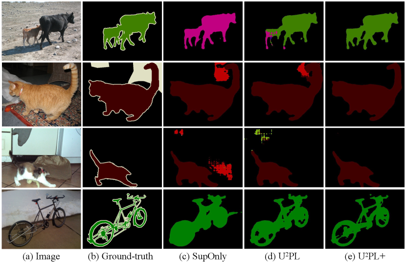
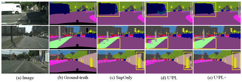
Fig. 4 and Fig. 5 show the results of different methods on the PASCAL VOC 2012 val set and Cityscapes val set, respectively. Benefiting from using unreliable pseudo-labels, UPL+ outperforms the supervised baseline, and UPL+ is able to generate a more accurate segmentation map.
Furthermore, through visualizing the segmentation results, we find that our method achieves much better performance on those ambiguous regions (e.g., the border between different objects). Such visual difference proves that our method finally makes the reliability of unreliable prediction labels stronger.
| GTA5 Cityscapes | ||||||||||||||||||||
| Method |
Road |
S.walk |
Build. |
Wall |
Fence |
Pole |
T.light |
Sign |
Veget. |
Terrain |
Sky |
Person |
Rider |
Car |
Truck |
Bus |
Train |
M.bike |
Bike |
mIoU |
| AdaptSeg | 86.5 | 25.9 | 79.8 | 22.1 | 20.0 | 23.6 | 33.1 | 21.8 | 81.8 | 25.9 | 75.9 | 57.3 | 26.2 | 76.3 | 29.8 | 32.1 | 7.2 | 29.5 | 32.5 | 41.4 |
| CyCADA | 86.7 | 35.6 | 80.1 | 19.8 | 17.5 | 38.0 | 39.9 | 41.5 | 82.7 | 27.9 | 73.6 | 64.9 | 19.0 | 65.0 | 12.0 | 28.6 | 4.5 | 31.1 | 42.0 | 42.7 |
| ADVENT | 89.4 | 33.1 | 81.0 | 26.6 | 26.8 | 27.2 | 33.5 | 24.7 | 83.9 | 36.7 | 78.8 | 58.7 | 30.5 | 84.8 | 38.5 | 44.5 | 1.7 | 31.6 | 32.4 | 45.5 |
| CBST | 91.8 | 53.5 | 80.5 | 32.7 | 21.0 | 34.0 | 28.9 | 20.4 | 83.9 | 34.2 | 80.9 | 53.1 | 24.0 | 82.7 | 30.3 | 35.9 | 16.0 | 25.9 | 42.8 | 45.9 |
| FADA | 92.5 | 47.5 | 85.1 | 37.6 | 32.8 | 33.4 | 33.8 | 18.4 | 85.3 | 37.7 | 83.5 | 63.2 | 39.7 | 87.5 | 32.9 | 47.8 | 1.6 | 34.9 | 39.5 | 49.2 |
| CAG_DA | 90.4 | 51.6 | 83.8 | 34.2 | 27.8 | 38.4 | 25.3 | 48.4 | 85.4 | 38.2 | 78.1 | 58.6 | 34.6 | 84.7 | 21.9 | 42.7 | 41.1 | 29.3 | 37.2 | 50.2 |
| FDA | 92.5 | 53.3 | 82.4 | 26.5 | 27.6 | 36.4 | 40.6 | 38.9 | 82.3 | 39.8 | 78.0 | 62.6 | 34.4 | 84.9 | 34.1 | 53.1 | 16.9 | 27.7 | 46.4 | 50.5 |
| PIT | 87.5 | 43.4 | 78.8 | 31.2 | 30.2 | 36.3 | 39.3 | 42.0 | 79.2 | 37.1 | 79.3 | 65.4 | 37.5 | 83.2 | 46.0 | 45.6 | 25.7 | 23.5 | 49.9 | 50.6 |
| IAST | 93.8 | 57.8 | 85.1 | 39.5 | 26.7 | 26.2 | 43.1 | 34.7 | 84.9 | 32.9 | 88.0 | 62.6 | 29.0 | 87.3 | 39.2 | 49.6 | 23.2 | 34.7 | 39.6 | 51.5 |
| ProDA | 91.5 | 52.4 | 82.9 | 42.0 | 35.7 | 40.0 | 44.4 | 43.3 | 87.0 | 43.8 | 79.5 | 66.5 | 31.4 | 86.7 | 41.1 | 52.5 | 0.0 | 45.4 | 53.8 | 53.7 |
| DAFormer | 95.7 | 70.2 | 89.4 | 53.5 | 48.1 | 49.6 | 55.8 | 59.4 | 89.9 | 47.9 | 92.5 | 72.2 | 44.7 | 92.3 | 74.5 | 78.2 | 65.1 | 55.9 | 61.8 | 68.3 |
| UPL+ | 95.7 | 70.9 | 89.7 | 53.3 | 46.3 | 47.0 | 59.1 | 58.3 | 90.4 | 48.6 | 92.9 | 73.2 | 44.6 | 92.6 | 77.5 | 77.8 | 76.7 | 59.3 | 67.5 | 69.6 |
| SYNTHIA Cityscapes | ||||||||||||||||||||
| Method |
Road |
S.walk |
Build. |
Wall |
Fence |
Pole |
T.light |
Sign |
Veget. |
Terrain |
Sky |
Person |
Rider |
Car |
Truck |
Bus |
Train |
M.bike |
Bike |
mIoU16 |
| ADVENT | 85.6 | 42.2 | 79.7 | 8.7 | 0.4 | 25.9 | 5.4 | 8.1 | 80.4 | - | 84.1 | 57.9 | 23.8 | 73.3 | - | 36.4 | - | 14.2 | 33.0 | 41.2 |
| CBST | 68.0 | 29.9 | 76.3 | 10.8 | 1.4 | 33.9 | 22.8 | 29.5 | 77.6 | - | 78.3 | 60.6 | 28.3 | 81.6 | - | 23.5 | - | 18.8 | 39.8 | 42.6 |
| CAG_DA | 84.7 | 40.8 | 81.7 | 7.8 | 0.0 | 35.1 | 13.3 | 22.7 | 84.5 | - | 77.6 | 64.2 | 27.8 | 80.9 | - | 19.7 | - | 22.7 | 48.3 | 44.5 |
| PIT | 83.1 | 27.6 | 81.5 | 8.9 | 0.3 | 21.8 | 26.4 | 33.8 | 76.4 | - | 78.8 | 64.2 | 27.6 | 79.6 | - | 31.2 | - | 31.0 | 31.3 | 44.0 |
| FADA | 84.5 | 40.1 | 83.1 | 4.8 | 0.0 | 34.3 | 20.1 | 27.2 | 84.8 | - | 84.0 | 53.5 | 22.6 | 85.4 | - | 43.7 | - | 26.8 | 27.8 | 45.2 |
| PyCDA | 75.5 | 30.9 | 83.3 | 20.8 | 0.7 | 32.7 | 27.3 | 33.5 | 84.7 | - | 85.0 | 64.1 | 25.4 | 85.0 | - | 45.2 | - | 21.2 | 32.0 | 46.7 |
| IAST | 81.9 | 41.5 | 83.3 | 17.7 | 4.6 | 32.3 | 30.9 | 28.8 | 83.4 | - | 85.0 | 65.5 | 30.8 | 86.5 | - | 38.2 | - | 33.1 | 52.7 | 49.8 |
| SAC | 89.3 | 47.2 | 85.5 | 26.5 | 1.3 | 43.0 | 45.5 | 32.0 | 87.1 | - | 89.3 | 63.6 | 25.4 | 86.9 | - | 35.6 | - | 30.4 | 53.0 | 52.6 |
| ProDA | 87.1 | 44.0 | 83.2 | 26.9 | 0.7 | 42.0 | 45.8 | 34.2 | 86.7 | - | 81.3 | 68.4 | 22.1 | 87.7 | - | 50.0 | - | 31.4 | 38.6 | 51.9 |
| DAFormer | 84.5 | 40.7 | 88.4 | 41.5 | 6.5 | 50.0 | 55.0 | 54.6 | 86.0 | - | 89.8 | 73.2 | 48.2 | 87.2 | - | 53.2 | - | 53.9 | 61.7 | 60.9 |
| UPL+ | 85.3 | 45.7 | 87.6 | 42.8 | 5.0 | 41.9 | 57.8 | 49.4 | 86.8 | - | 89.9 | 75.8 | 49.0 | 88.0 | - | 61.6 | - | 54.1 | 64.8 | 61.6 |
4.2 Experiments on Domain Adaptive Segmentation
In this section, we evaluate the efficacy of our UPL+ under the domain adaptation (DA) setting. Different from semi-supervised learning, DA often suffers from a domain shift between labeled source domain and unlabeled target domain (Hoyer et al., , 2022; Zhang et al., 2021b, ; Li et al., 2022b, ; Chen et al., , 2019; Hoffman et al., , 2018; Li et al., , 2019; Luo et al., , 2019), which is more important to make sufficient use of all pseudo-labels. We first describe experimental settings for domain adaptive semantic segmentation. Then, we compare our UPL+ with state-of-the-art alternatives. Finally, we provide qualitative results.
Datasets.
In this setting, we use synthetic images from either GTA5 (Richter et al., , 2016) or SYNTHIA (Ros et al., , 2016) as the source domain and use real-world images from Cityscapes (Cordts et al., , 2016) as the target domain. GTA5 (Richter et al., , 2016) consists of images with resolution , and SYNTHIA (Ros et al., , 2016) contains images with resolution .
Network Structure.
Evaluation Metric.
For the DA segmentation task, we report results on the Cityscapes val set. Particularly, on SYNTHIA Cityscapes DA benchmark, 16 of the 19 classes of Cityscapes are used to calculate mIoU, following the common practice (Hoyer et al., , 2022).
| GTA5 Cityscapes | SYNTHIA Cityscapes | |||
| R | U | mIoU | mIoU16 | |
| ✓ | 68.4 | 60.8 | ||
| ✓ | 68.6 | 60.9 | ||
| ✓ | 69.3 | 61.2 | ||
| ✓ | ✓ | 68.7 | 60.9 | |
| ✓ | ✓ | 69.6 | 61.6 | |
| ✓ | ✓ | ✓ | 68.5 | 60.8 |
| GTA5 Cityscapes | ||||||||||
| Method |
Wall |
T.light |
Sign |
Rider |
Truck |
Bus |
Train |
M.bike |
Bike |
mIoU |
| DAFormer | 53.5 | 55.8 | 59.4 | 44.7 | 74.5 | 78.2 | 65.1 | 55.9 | 61.8 | 60.9 |
| UPL+ | 53.3 | 59.1 | 58.3 | 44.6 | 77.5 | 77.8 | 76.7 | 59.3 | 67.5 | 63.8 |
Implementation Details.
Following previous methods (Zhang et al., 2021b, ; Hoyer et al., , 2022), we first resize the images to for Cityscapes and for GTA5, and then randomly crop them into for training. For the testing stage, we just resize the images to . We use AdamW (Loshchilov and Hutter, , 2017) optimizer with weight decay of and initial learning rate for the encoder and for the decoder follow (Hoyer et al., , 2022). In accordance with DAFormer (Hoyer et al., , 2022), we warm up the learning rate in a linear schedule with k steps and linear decay since then. In total, the model is trained with a batch of one labeled source image and one unlabeled target image for k iterations. We adopt DAFormer (Hoyer et al., , 2022) as our baseline and apply extra contrastive learning with our sample strategy. We evaluate our proposed UPL+ under two DA benchmarks (i.e., GTA5 Cityscapes and SYNTHIA Cityscapes). All DA experiments are conducted with a single Tesla A100 GPU.
Comparisons with State-of-the-Art Alternatives.
We compare our proposed UPL+ with state-of-the-art alternatives, including adversarial training methods (AdaptSeg (Tsai et al., , 2018), CyCADA (Hoffman et al., , 2018), FADA (Wang et al., 2020a, ), and ADVENT (Vu et al., , 2019)), and self-training methods (CBST (Zou et al., , 2018), IAST (Mei et al., , 2020), CAG_DA (Zhang et al., , 2019), ProDA (Zhang et al., 2021b, ), CPSL (Li et al., 2022b, ), SAC (Araslanov and Roth, , 2021), and DAFormer (Hoyer et al., , 2022)).
GTA5 Cityscapes.
As shown in Tab. 13, our proposed UPL+ achieves the best IoU performance on 13 out of 19 categories, and the IoU scores of the remaining 6 classes rank second. Its mIoU is and outperforms DAFormer (Hoyer et al., , 2022) by . Since DAFormer (Hoyer et al., , 2022) is our baseline, the results prove that mining all unreliable pseudo-labels do help the model. Note that there is no need to apply knowledge distillation as ProDA (Zhang et al., 2021b, ) and CPSL (Li et al., 2022b, ) do, which incarnates the efficiency and simplicity of our method and the robustness of our core insight. From Tab. 13, we can tell that by introducing unreliable pseudo-labels into training, UPL+ attains IoU on class train, where ProDA (Zhang et al., 2021b, ), FADA (Wang et al., 2020a, ), and ADVENT (Vu et al., , 2019) even fail on this difficult long-tailed class.
SYNTHIA Cityscapes.
This DA task is more challenging than GTA5 Cityscapes due to the larger domain gap between the labeled source domain and the unlabeled target domain. As shown in Tab. 13, our proposed UPL+ achieves the best IoU performance on 8 out of 16 categories, and the mIoU over 16 classes (mIoU16) of our method outperforms other state-of-the-art alternatives, achieving . Specifically, UPL+ performs especially great on class bus, which surpasses DAFormer (Hoyer et al., , 2022) by a large margin of .
Effectiveness of Using Unreliable Pseudo-Labels.
We study our core insight, i.e., using unreliable pseudo-labels to promote domain adaptive semantic segmentation, we conduct experiments about selecting negative candidates with different reliability in Tab. 14. As illustrated in the table, containing features from the source domain brings marginal improvements. Significant improvements are brought because of the introduction of unreliable predictions.
Performance on Tailed Classes.
From Tab. 15, we can tell that the improvements of our UPL+ on tailed classes are much more significant than those of all categories. For instance, on the GTA5 Cityscapes benchmark, UPL+ outperforms DAFormer (Hoyer et al., , 2022) by +1.3 mIoU (69.6 v.s. 68.3) and +2.9 mIoUtail (63.8 v.s. 60.9), respectively.
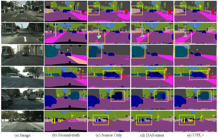
Qualitative Results.
Discussion.
Both DA and SS aim at leveraging a large amount of unlabeled data, while DA often suffers from domain shift, and is more important to learn domain-invariant feature representations, building a cross-category-discriminative feature embedding space. Although our UPL+ mainly focuses on semi-supervised learning and does not pay much attention to bridging the gap between source and target domains, using unreliable pseudo-labels provides another efficient way for generalization. This might be because, in DA, the quality of pseudo-labels is much worse than those in SS due to the limited generalization ability of the segmentation model, making sufficient use of all pixels remains a valuable issue hence.
4.3 Experiments on Weakly Supervised Segmentation
| Method | Sup. | Backbone | val | test |
| Fully Supervised Methods | ||||
| DeepLab | ResNet-101 | 77.6 | 79.7 | |
| WideResNet38 | WR-38 | 80.8 | 82.5 | |
| SegFormer† | MiT-B1 | 78.7 | ||
| Multi-Stage Weakly Supervised Methods | ||||
| OAA+ | ResNet-101 | 65.2 | 66.4 | |
| MCIS | ResNet-101 | 66.2 | 66.9 | |
| AuxSegNet | WR-38 | 69.0 | 68.6 | |
| NSROM | ResNet-101 | 70.4 | 70.2 | |
| EPS | ResNet-101 | 70.9 | 70.8 | |
| SEAM | WR-38 | 64.5 | 65.7 | |
| SC-CAM | ResNet-101 | 66.1 | 65.9 | |
| CDA | WR-38 | 66.1 | 66.8 | |
| AdvCAM | ResNet-101 | 68.1 | 68.0 | |
| CPN | ResNet-101 | 67.8 | 68.5 | |
| RIB | ResNet-101 | 68.3 | 68.6 | |
| Single-Stage Weakly Supervised Methods | ||||
| EM | VGG-16 | 38.2 | 39.6 | |
| MIL | 42.0 | 40.6 | ||
| CRF-RNN | VGG-16 | 52.8 | 53.7 | |
| RRM | WR-38 | 62.6 | 62.9 | |
| 1Stage | WR-38 | 62.7 | 64.3 | |
| AFA† | MiT-B1 | 64.9 | 66.1 | |
| UPL+ | MiT-B1 | 66.4 | 67.0 | |
| mIoU | ||
| ✓ | 65.0 | |
| ✓ | 65.7 | |
| ✓ | ✓ | 66.4 |
In this section, we evaluate the efficacy of our UPL+ under the weakly supervised (WS) setting. Differently, under this setting, pixel-level annotations are entirely inaccessible, what we have is only image-level labels, making it crucial to make sufficient use of all pixel-level predictions. We first describe experimental settings for domain adaptive semantic segmentation. Then, we compare our UPL+ with state-of-the-art alternatives. Finally, we provide qualitative results.
Several WS methods with image-level labels adopt a multi-stage framework, e.g., (Jiang et al., , 2019; Sun et al., , 2020). They first train a classification model and generate CAMs to be pseudo-labels. Additional refinement techniques are usually required to improve the quality of these pseudo-labels. Finally, a standalone semantic segmentation network is trained using these pseudo-labels. This type of training pipeline is obviously not efficient. To this end, we select a representative single-stage method, AFA (Ru et al., , 2022) as the baseline, where the final segmentation model is trained end-to-end.
Datasets.
In this setting, we conduct experiments on PASCAL VOC 2012 (Everingham et al., , 2010), which contains 21 semantic classes (including the background class). Following common practices (Fan et al., 2020c, ; Fan et al., 2020b, ; Fan et al., 2020a, ), it is augmented with the SBD dataset (Hariharan et al., , 2011), resulting in , , and images for training, validation, and testing, respectively.
Network Structure.
We take AFA (Ru et al., , 2022) as the baseline, which uses the Mix Transformer (MiT) (Xie et al., , 2021) as the backbone. A simple MLP head is used to be the segmentation head following (Xie et al., , 2021). The backbone is pre-trained on ImageNet-1K (Deng et al., , 2009), while other parameters are randomly initialized. The representation head is the same as in the semi-supervised setting.
Evaluation Metric.
By default, we report the mIoU on both the validation set and testing set as the evaluation criteria.
Implementation Details.
Following the standard configuration of AFA (Ru et al., , 2022), the AdamW optimizer is used to train the model, whose initial learning rate is set to and decays every iteration with a polynomial scheduler for parameters of the backbone. The learning rates for other parameters are ten times that of the backbone. The weight decay is fixed at . Random rescaling with a range of , random horizontal flipping, and random cropping with a cropping size of are adopted. The network for iterations with a batch size of . All WS experiments are conducted with 2080Ti GPUs.
Comparisons with State-of-the-Art Alternatives.
In Tab. 16, we compare our proposed UPL+ with a wide range of representative state-of-the-art alternatives, including multi-stage methods and single-stage methods. Some multi-stage methods further leverage saliency maps, including OAA+ (Jiang et al., , 2019), MCIS (Sun et al., , 2020), AuxSegNet (Xu et al., 2021a, ), NSROM (Yao et al., , 2021), and EPS (Lee et al., 2021c, ), while others do not, including SEAM (Wang et al., 2020b, ), SC-CAM (Chang et al., , 2020), CDA (Su et al., , 2021), AdvCAM (Lee et al., 2021b, ), CPN (Zhang et al., 2021a, ), and RIB (Lee et al., 2021a, ). Single-stage methods include EM (Papandreou et al., , 2015), MIL (Pinheiro and Collobert, , 2015), CRF-RNN (Roy and Todorovic, , 2017), RRM (Zhang et al., 2020a, ), 1Stage (Araslanov and Roth, , 2020), and AFA (Ru et al., , 2022). All methods are refined using CRF.
It has been illustrated in Tab. 16 that UPL+ brings improvements of mIoU and mIoU over AFA (Ru et al., , 2022) on the val set and the test set, respectively. UPL+ clearly surpasses previous state-of-the-art single-stage methods with significant margins. It is worth noticing that UPL+ manages to achieve competitive results even when compared with multi-stage methods, e.g., OAA+ (Jiang et al., , 2019), MCIS (Sun et al., , 2020), SEAM (Wang et al., 2020b, ), SC-CAM (Chang et al., , 2020) and CDA (Su et al., , 2021).
Effectiveness of Using Unreliable Pseudo-Labels.
We study our core insight, i.e., using unreliable pseudo-labels promotes weakly supervised semantic segmentation, we conduct experiments about selecting negative candidates with different reliability in Tab. 17. As illustrated in the table, incorporating unreliable predictions, i.e., , brings significant improvements. It is worth noticing that since we do not have any dense annotations, and thus leveraging the image-level annotations, i.e., , in selecting negative candidates becomes crucial for a stable training procedure.
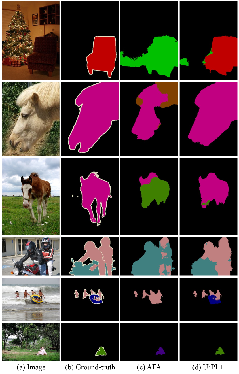
Qualitative Results.
5 Conclusion
In this paper, we extend our original U2PL to UPL+, a unified framework for label-efficient semantic segmentation, by including unreliable pseudo-labels into training. Our main insight is that those unreliable predictions are usually just confused about a few classes and are confident enough not to belong to the remaining remote classes. UPL+ outperforms many existing state-of-the-art methods in both semi-supervised, domain adaptive, and weakly supervised semantic segmentation, suggesting our framework provides a new promising paradigm in label-efficient learning research. Our ablation experiments prove the insight of this work is quite solid, i.e., only when introducing unreliable predictions into the contrastive learning paradigm brings significant improvements under both settings. Qualitative results give visual proof of its effectiveness, especially the better performance on borders between semantic objects or other ambiguous regions.
Declarations
Acknowledgements This work was supported in part by the National Key R&D Program of China (No. 2022ZD0116500), the National Natural Science Foundation of China (No. U21B2042), and in part by the 2035 Innovation Program of CAS, and the InnoHK program.
Data Availability. The datasets generated during and/or analyzed during the current study are available from the PASCAL VOC 2012111http://host.robots.ox.ac.uk/pascal/VOC/, the SBD222https://ieeexplore.ieee.org/abstract/document/6126343, the GTA5333https://arxiv.org/pdf/1608.02192v1.pdf, the Synthia444https://synthia-dataset.net/, and the Cityscapes555https://www.cityscapes-dataset.com/.
References
- Abramov et al., (2020) Abramov, A., Bayer, C., and Heller, C. (2020). Keep it simple: Image statistics matching for domain adaptation. arXiv preprint arXiv:2005.12551.
- Ahn and Kwak, (2018) Ahn, J. and Kwak, S. (2018). Learning pixel-level semantic affinity with image-level supervision for weakly supervised semantic segmentation. In CVPR.
- Alonso et al., (2021) Alonso, I., Sabater, A., Ferstl, D., Montesano, L., and Murillo, A. C. (2021). Semi-supervised semantic segmentation with pixel-level contrastive learning from a class-wise memory bank. In ICCV.
- Araslanov and Roth, (2020) Araslanov, N. and Roth, S. (2020). Single-stage semantic segmentation from image labels. In CVPR.
- Araslanov and Roth, (2021) Araslanov, N. and Roth, S. (2021). Self-supervised augmentation consistency for adapting semantic segmentation. In CVPR.
- Arazo et al., (2020) Arazo, E., Ortego, D., Albert, P., O’Connor, N. E., and McGuinness, K. (2020). Pseudo-labeling and confirmation bias in deep semi-supervised learning. In International Joint Conference on Neural Networks (IJCNN.
- Bachman et al., (2014) Bachman, P., Alsharif, O., and Precup, D. (2014). Learning with pseudo-ensembles. NeurIPS.
- Badrinarayanan et al., (2017) Badrinarayanan, V., Kendall, A., and Cipolla, R. (2017). Segnet: A deep convolutional encoder-decoder architecture for image segmentation. TPAMI, 39(12):2481–2495.
- Chang et al., (2019) Chang, W.-L., Wang, H.-P., Peng, W.-H., and Chiu, W.-C. (2019). All about structure: Adapting structural information across domains for boosting semantic segmentation. In CVPR.
- Chang et al., (2020) Chang, Y.-T., Wang, Q., Hung, W.-C., Piramuthu, R., Tsai, Y.-H., and Yang, M.-H. (2020). Weakly-supervised semantic segmentation via sub-category exploration. In CVPR.
- Chen et al., (2019) Chen, C., Xie, W., Huang, W., Rong, Y., Ding, X., Huang, Y., Xu, T., and Huang, J. (2019). Progressive feature alignment for unsupervised domain adaptation. In CVPR.
- (12) Chen, H., Jin, Y., Jin, G., Zhu, C., and Chen, E. (2021a). Semi-supervised semantic segmentation by improving prediction confidence. IEEE Transactions on Neural Networks and Learning Systems, 13(1).
- (13) Chen, L.-C., Papandreou, G., Kokkinos, I., Murphy, K., and Yuille, A. L. (2017a). Deeplab: Semantic image segmentation with deep convolutional nets, atrous convolution, and fully connected crfs. TPAMI, 40(4):834–848.
- (14) Chen, L.-C., Papandreou, G., Schroff, F., and Adam, H. (2017b). Rethinking atrous convolution for semantic image segmentation. arXiv preprint arXiv:1706.05587.
- Chen et al., (2018) Chen, L.-C., Zhu, Y., Papandreou, G., Schroff, F., and Adam, H. (2018). Encoder-decoder with atrous separable convolution for semantic image segmentation. In ECCV.
- Chen et al., (2020) Chen, T., Kornblith, S., Swersky, K., Norouzi, M., and Hinton, G. (2020). Big self-supervised models are strong semi-supervised learners. NeurIPS.
- (17) Chen, X., Xie, S., and He, K. (2021b). An empirical study of training self-supervised vision transformers. In ICCV.
- (18) Chen, X., Yuan, Y., Zeng, G., and Wang, J. (2021c). Semi-supervised semantic segmentation with cross pseudo supervision. In CVPR.
- Cheng et al., (2022) Cheng, B., Misra, I., Schwing, A. G., Kirillov, A., and Girdhar, R. (2022). Masked-attention mask transformer for universal image segmentation. In CVPR.
- Cheng et al., (2021) Cheng, B., Schwing, A., and Kirillov, A. (2021). Per-pixel classification is not all you need for semantic segmentation. NeurIPS.
- Choi et al., (2019) Choi, J., Kim, T., and Kim, C. (2019). Self-ensembling with gan-based data augmentation for domain adaptation in semantic segmentation. In ICCV.
- Cordts et al., (2016) Cordts, M., Omran, M., Ramos, S., Rehfeld, T., Enzweiler, M., Benenson, R., Franke, U., Roth, S., and Schiele, B. (2016). The cityscapes dataset for semantic urban scene understanding. In CVPR.
- Dai et al., (2015) Dai, J., He, K., and Sun, J. (2015). Boxsup: Exploiting bounding boxes to supervise convolutional networks for semantic segmentation. In ICCV.
- Deng et al., (2009) Deng, J., Dong, W., Socher, R., Li, L.-J., Li, K., and Fei-Fei, L. (2009). Imagenet: A large-scale hierarchical image database. In CVPR.
- DeVries and Taylor, (2017) DeVries, T. and Taylor, G. W. (2017). Improved regularization of convolutional neural networks with cutout. arXiv preprint arXiv:1708.04552.
- Dosovitskiy et al., (2021) Dosovitskiy, A., Beyer, L., Kolesnikov, A., Weissenborn, D., Zhai, X., Unterthiner, T., Dehghani, M., Minderer, M., Heigold, G., Gelly, S., et al. (2021). An image is worth 16x16 words: Transformers for image recognition at scale. In ICLR.
- (27) Du, Y., Fu, Z., Liu, Q., and Wang, Y. (2022a). Weakly supervised semantic segmentation by pixel-to-prototype contrast. In CVPR.
- (28) Du, Y., Shen, Y., Wang, H., Fei, J., Li, W., Wu, L., Zhao, R., Fu, Z., and Liu, Q. (2022b). Learning from future: A novel self-training framework for semantic segmentation. NeurIPS.
- Everingham et al., (2010) Everingham, M., Van Gool, L., Williams, C. K., Winn, J., and Zisserman, A. (2010). The pascal visual object classes (voc) challenge. IJCV, 88(2):303–338.
- (30) Fan, J., Zhang, Z., Song, C., and Tan, T. (2020a). Learning integral objects with intra-class discriminator for weakly-supervised semantic segmentation. In CVPR.
- (31) Fan, J., Zhang, Z., and Tan, T. (2020b). Employing multi-estimations for weakly-supervised semantic segmentation. In ECCV.
- Fan et al., (2022) Fan, J., Zhang, Z., and Tan, T. (2022). Pointly-supervised panoptic segmentation. In ECCV. Springer.
- (33) Fan, J., Zhang, Z., Tan, T., Song, C., and Xiao, J. (2020c). Cian: Cross-image affinity net for weakly supervised semantic segmentation. In AAAI.
- French et al., (2020) French, G., Laine, S., Aila, T., Mackiewicz, M., and Finlayson, G. (2020). Semi-supervised semantic segmentation needs strong, varied perturbations. In BMVC.
- Gong et al., (2019) Gong, R., Li, W., Chen, Y., and Gool, L. V. (2019). Dlow: Domain flow for adaptation and generalization. In CVPR.
- Goodfellow et al., (2014) Goodfellow, I., Pouget-Abadie, J., Mirza, M., Xu, B., Warde-Farley, D., Ozair, S., Courville, A., and Bengio, Y. (2014). Generative adversarial nets. NeurIPS.
- Grandvalet and Bengio, (2004) Grandvalet, Y. and Bengio, Y. (2004). Semi-supervised learning by entropy minimization. NeurIPS.
- Hariharan et al., (2011) Hariharan, B., Arbeláez, P., Bourdev, L., Maji, S., and Malik, J. (2011). Semantic contours from inverse detectors. In ICCV.
- He et al., (2020) He, K., Fan, H., Wu, Y., Xie, S., and Girshick, R. (2020). Momentum contrast for unsupervised visual representation learning. In CVPR.
- He et al., (2016) He, K., Zhang, X., Ren, S., and Sun, J. (2016). Deep residual learning for image recognition. In CVPR.
- Hoffman et al., (2018) Hoffman, J., Tzeng, E., Park, T., Zhu, J.-Y., Isola, P., Saenko, K., Efros, A., and Darrell, T. (2018). Cycada: Cycle-consistent adversarial domain adaptation. In ICML.
- Hoffman et al., (2016) Hoffman, J., Wang, D., Yu, F., and Darrell, T. (2016). Fcns in the wild: Pixel-level adversarial and constraint-based adaptation. arXiv preprint arXiv:1612.02649.
- Hong et al., (2018) Hong, W., Wang, Z., Yang, M., and Yuan, J. (2018). Conditional generative adversarial network for structured domain adaptation. In CVPR.
- Hoyer et al., (2022) Hoyer, L., Dai, D., and Van Gool, L. (2022). Daformer: Improving network architectures and training strategies for domain-adaptive semantic segmentation. In CVPR.
- Hu et al., (2021) Hu, H., Wei, F., Hu, H., Ye, Q., Cui, J., and Wang, L. (2021). Semi-supervised semantic segmentation via adaptive equalization learning. NeurIPS.
- Ji et al., (2023) Ji, W., Li, J., Bi, Q., Liu, T., Li, W., and Cheng, L. (2023). Segment anything is not always perfect: An investigation of sam on different real-world applications. arXiv preprint arXiv:2304.05750.
- Jiang et al., (2019) Jiang, P.-T., Hou, Q., Cao, Y., Cheng, M.-M., Wei, Y., and Xiong, H.-K. (2019). Integral object mining via online attention accumulation. In ICCV.
- Kang et al., (2020) Kang, G., Wei, Y., Yang, Y., Zhuang, Y., and Hauptmann, A. (2020). Pixel-level cycle association: A new perspective for domain adaptive semantic segmentation. NeurIPS.
- Ke et al., (2020) Ke, Z., Qiu, D., Li, K., Yan, Q., and Lau, R. W. (2020). Guided collaborative training for pixel-wise semi-supervised learning. In ECCV.
- Kim et al., (2021) Kim, B., Han, S., and Kim, J. (2021). Discriminative region suppression for weakly-supervised semantic segmentation. In AAAI.
- Kirillov et al., (2023) Kirillov, A., Mintun, E., Ravi, N., Mao, H., Rolland, C., Gustafson, L., Xiao, T., Whitehead, S., Berg, A. C., Lo, W.-Y., et al. (2023). Segment anything. In ICCV.
- Krähenbühl and Koltun, (2011) Krähenbühl, P. and Koltun, V. (2011). Efficient inference in fully connected crfs with gaussian edge potentials. NeurIPS.
- Krizhevsky et al., (2009) Krizhevsky, A., Hinton, G., et al. (2009). Learning multiple layers of features from tiny images.
- (54) Lee, C.-Y., Batra, T., Baig, M. H., and Ulbricht, D. (2019a). Sliced wasserstein discrepancy for unsupervised domain adaptation. In CVPR.
- Lee et al., (2013) Lee, D.-H. et al. (2013). Pseudo-label: The simple and efficient semi-supervised learning method for deep neural networks. In ICML, volume 3, page 896.
- (56) Lee, J., Choi, J., Mok, J., and Yoon, S. (2021a). Reducing information bottleneck for weakly supervised semantic segmentation. NeurIPS.
- (57) Lee, J., Kim, E., Lee, S., Lee, J., and Yoon, S. (2019b). Ficklenet: Weakly and semi-supervised semantic image segmentation using stochastic inference. In CVPR.
- (58) Lee, J., Kim, E., and Yoon, S. (2021b). Anti-adversarially manipulated attributions for weakly and semi-supervised semantic segmentation. In CVPR.
- (59) Lee, S., Lee, M., Lee, J., and Shim, H. (2021c). Railroad is not a train: Saliency as pseudo-pixel supervision for weakly supervised semantic segmentation. In CVPR.
- (60) Li, J., Fan, J., and Zhang, Z. (2022a). Towards noiseless object contours for weakly supervised semantic segmentation. In CVPR.
- (61) Li, R., Jia, X., He, J., Chen, S., and Hu, Q. (2021a). T-svdnet: Exploring high-order prototypical correlations for multi-source domain adaptation. In ICCV.
- (62) Li, R., Li, S., He, C., Zhang, Y., Jia, X., and Zhang, L. (2022b). Class-balanced pixel-level self-labeling for domain adaptive semantic segmentation. In CVPR.
- (63) Li, Y., Kuang, Z., Liu, L., Chen, Y., and Zhang, W. (2021b). Pseudo-mask matters in weakly-supervised semantic segmentation. In ICCV.
- Li et al., (2019) Li, Y., Yuan, L., and Vasconcelos, N. (2019). Bidirectional learning for domain adaptation of semantic segmentation. In CVPR.
- Lin et al., (2016) Lin, D., Dai, J., Jia, J., He, K., and Sun, J. (2016). Scribblesup: Scribble-supervised convolutional networks for semantic segmentation. In CVPR.
- Liu et al., (2021) Liu, S., Zhi, S., Johns, E., and Davison, A. J. (2021). Bootstrapping semantic segmentation with regional contrast. arXiv preprint arXiv:2104.04465.
- (67) Long, J., Shelhamer, E., and Darrell, T. (2015a). Fully convolutional networks for semantic segmentation. In CVPR.
- (68) Long, M., Cao, Y., Wang, J., and Jordan, M. (2015b). Learning transferable features with deep adaptation networks. In ICML.
- Loshchilov and Hutter, (2017) Loshchilov, I. and Hutter, F. (2017). Decoupled weight decay regularization. arXiv preprint arXiv:1711.05101.
- Luo et al., (2019) Luo, Y., Zheng, L., Guan, T., Yu, J., and Yang, Y. (2019). Taking a closer look at domain shift: Category-level adversaries for semantics consistent domain adaptation. In CVPR.
- Ma et al., (2024) Ma, J., He, Y., Li, F., Han, L., You, C., and Wang, B. (2024). Segment anything in medical images. Nature Communications, 15(1):654.
- Mei et al., (2020) Mei, K., Zhu, C., Zou, J., and Zhang, S. (2020). Instance adaptive self-training for unsupervised domain adaptation. In ECCV.
- Melas-Kyriazi and Manrai, (2021) Melas-Kyriazi, L. and Manrai, A. K. (2021). Pixmatch: Unsupervised domain adaptation via pixelwise consistency training. In CVPR.
- Murez et al., (2018) Murez, Z., Kolouri, S., Kriegman, D., Ramamoorthi, R., and Kim, K. (2018). Image to image translation for domain adaptation. In CVPR.
- Nowozin et al., (2016) Nowozin, S., Cseke, B., and Tomioka, R. (2016). f-gan: Training generative neural samplers using variational divergence minimization. NeurIPS.
- Olsson et al., (2021) Olsson, V., Tranheden, W., Pinto, J., and Svensson, L. (2021). Classmix: Segmentation-based data augmentation for semi-supervised learning. In CVPR.
- Oord et al., (2018) Oord, A. v. d., Li, Y., and Vinyals, O. (2018). Representation learning with contrastive predictive coding. arXiv preprint arXiv:1807.03748.
- Ouali et al., (2020) Ouali, Y., Hudelot, C., and Tami, M. (2020). Semi-supervised semantic segmentation with cross-consistency training. In CVPR.
- Papandreou et al., (2015) Papandreou, G., Chen, L.-C., Murphy, K. P., and Yuille, A. L. (2015). Weakly-and semi-supervised learning of a deep convolutional network for semantic image segmentation. In ICCV.
- Pinheiro and Collobert, (2015) Pinheiro, P. O. and Collobert, R. (2015). From image-level to pixel-level labeling with convolutional networks. In CVPR.
- Richter et al., (2016) Richter, S. R., Vineet, V., Roth, S., and Koltun, V. (2016). Playing for data: Ground truth from computer games. In ECCV.
- Ronneberger et al., (2015) Ronneberger, O., Fischer, P., and Brox, T. (2015). U-net: Convolutional networks for biomedical image segmentation. In International Conference on Medical Image Computing and Computer Assisted Intervention, pages 234–241. Springer.
- Ros et al., (2016) Ros, G., Sellart, L., Materzynska, J., Vazquez, D., and Lopez, A. M. (2016). The synthia dataset: A large collection of synthetic images for semantic segmentation of urban scenes. In CVPR.
- Roy and Todorovic, (2017) Roy, A. and Todorovic, S. (2017). Combining bottom-up, top-down, and smoothness cues for weakly supervised image segmentation. In Proceedings of the IEEE conference on computer vision and pattern recognition, pages 3529–3538.
- Ru et al., (2022) Ru, L., Zhan, Y., Yu, B., and Du, B. (2022). Learning affinity from attention: end-to-end weakly-supervised semantic segmentation with transformers. In CVPR.
- Ru et al., (2023) Ru, L., Zheng, H., Zhan, Y., and Du, B. (2023). Token contrast for weakly-supervised semantic segmentation. In CVPR.
- Saito et al., (2018) Saito, K., Watanabe, K., Ushiku, Y., and Harada, T. (2018). Maximum classifier discrepancy for unsupervised domain adaptation. In CVPR.
- Sajjadi et al., (2016) Sajjadi, M., Javanmardi, M., and Tasdizen, T. (2016). Regularization with stochastic transformations and perturbations for deep semi-supervised learning. NeurIPS.
- Sakaridis et al., (2021) Sakaridis, C., Dai, D., and Van Gool, L. (2021). Acdc: The adverse conditions dataset with correspondences for semantic driving scene understanding. In ICCV.
- Sankaranarayanan et al., (2018) Sankaranarayanan, S., Balaji, Y., Jain, A., Lim, S. N., and Chellappa, R. (2018). Learning from synthetic data: Addressing domain shift for semantic segmentation. In CVPR.
- Sohn et al., (2020) Sohn, K., Berthelot, D., Carlini, N., Zhang, Z., Zhang, H., Raffel, C. A., Cubuk, E. D., Kurakin, A., and Li, C.-L. (2020). Fixmatch: Simplifying semi-supervised learning with consistency and confidence. NeurIPS.
- Strudel et al., (2021) Strudel, R., Garcia, R., Laptev, I., and Schmid, C. (2021). Segmenter: Transformer for semantic segmentation. In ICCV.
- Su et al., (2021) Su, Y., Sun, R., Lin, G., and Wu, Q. (2021). Context decoupling augmentation for weakly supervised semantic segmentation. In ICCV.
- Sun et al., (2020) Sun, G., Wang, W., Dai, J., and Van Gool, L. (2020). Mining cross-image semantics for weakly supervised semantic segmentation. In ECCV. Springer.
- Sun et al., (2021) Sun, K., Shi, H., Zhang, Z., and Huang, Y. (2021). Ecs-net: Improving weakly supervised semantic segmentation by using connections between class activation maps. In ICCV.
- Tarvainen and Valpola, (2017) Tarvainen, A. and Valpola, H. (2017). Mean teachers are better role models: Weight-averaged consistency targets improve semi-supervised deep learning results. NeurIPS.
- Tsai et al., (2018) Tsai, Y.-H., Hung, W.-C., Schulter, S., Sohn, K., Yang, M.-H., and Chandraker, M. (2018). Learning to adapt structured output space for semantic segmentation. In CVPR.
- Vu et al., (2019) Vu, T.-H., Jain, H., Bucher, M., Cord, M., and Pérez, P. (2019). Advent: Adversarial entropy minimization for domain adaptation in semantic segmentation. In CVPR.
- Wan et al., (2020) Wan, Z., Zhang, B., Chen, D., Zhang, P., Chen, D., Liao, J., and Wen, F. (2020). Bringing old photos back to life. In CVPR.
- (100) Wang, H., Fan, J., Wang, Y., Song, K., Wang, T., and Zhang, Z. (2023a). Droppos: Pre-training vision transformers by reconstructing dropped positions. Advances in Neural Information Processing Systems (NeurIPS).
- (101) Wang, H., Shen, T., Zhang, W., Duan, L.-Y., and Mei, T. (2020a). Classes matter: A fine-grained adversarial approach to cross-domain semantic segmentation. In ECCV.
- (102) Wang, H., Shen, Y., Fei, J., Li, W., Wu, L., Wang, Y., and Zhang, Z. (2023b). Pulling target to source: A new perspective on domain adaptive semantic segmentation. arXiv preprint arXiv:2305.13752.
- (103) Wang, H., Song, K., Fan, J., Wang, Y., Xie, J., and Zhang, Z. (2023c). Hard patches mining for masked image modeling. In CVPR.
- Wang et al., (2021) Wang, W., Zhou, T., Yu, F., Dai, J., Konukoglu, E., and Van Gool, L. (2021). Exploring cross-image pixel contrast for semantic segmentation. In ICCV.
- (105) Wang, Y., Chen, H., Fan, Y., Sun, W., Tao, R., Hou, W., Wang, R., Yang, L., Zhou, Z., Guo, L.-Z., Qi, H., Wu, Z., Li, Y.-F., Nakamura, S., Ye, W., Savvides, M., Raj, B., Shinozaki, T., Schiele, B., Wang, J., Xie, X., and Zhang, Y. (2022a). Usb: A unified semi-supervised learning benchmark for classification. In NeurIPS.
- (106) Wang, Y., Chen, H., Heng, Q., Hou, W., Fan, Y., Wu, Z., Wang, J., Savvides, M., Shinozaki, T., Raj, B., et al. (2023d). Freematch: Self-adaptive thresholding for semi-supervised learning. In ICLR.
- (107) Wang, Y., Fei, J., Wang, H., Li, W., Wu, L., Zhao, R., and Shen, Y. (2023e). Balancing logit variation for long-tail semantic segmentation. In CVPR.
- Wang et al., (2019) Wang, Y., Ma, X., Chen, Z., Luo, Y., Yi, J., and Bailey, J. (2019). Symmetric cross entropy for robust learning with noisy labels. In CVPR.
- (109) Wang, Y., Wang, H., Shen, Y., Fei, J., Li, W., Jin, G., Wu, L., Zhao, R., and Le, X. (2022b). Semi-supervised semantic segmentation using unreliable pseudo labels. In CVPR.
- (110) Wang, Y., Zhang, J., Kan, M., Shan, S., and Chen, X. (2020b). Self-supervised equivariant attention mechanism for weakly supervised semantic segmentation. In CVPR.
- Wei et al., (2017) Wei, Y., Feng, J., Liang, X., Cheng, M.-M., Zhao, Y., and Yan, S. (2017). Object region mining with adversarial erasing: A simple classification to semantic segmentation approach. In CVPR.
- Wu et al., (2021) Wu, T., Huang, J., Gao, G., Wei, X., Wei, X., Luo, X., and Liu, C. H. (2021). Embedded discriminative attention mechanism for weakly supervised semantic segmentation. In CVPR.
- Wu et al., (2019) Wu, Z., Wang, X., Gonzalez, J. E., Goldstein, T., and Davis, L. S. (2019). Ace: Adapting to changing environments for semantic segmentation. In ICCV.
- Xie et al., (2021) Xie, E., Wang, W., Yu, Z., Anandkumar, A., Alvarez, J. M., and Luo, P. (2021). Segformer: Simple and efficient design for semantic segmentation with transformers. NeurIPS.
- Xie et al., (2020) Xie, Q., Luong, M.-T., Hovy, E., and Le, Q. V. (2020). Self-training with noisy student improves imagenet classification. In CVPR.
- Xu et al., (2022) Xu, J., De Mello, S., Liu, S., Byeon, W., Breuel, T., Kautz, J., and Wang, X. (2022). Groupvit: Semantic segmentation emerges from text supervision. In CVPR.
- (117) Xu, L., Ouyang, W., Bennamoun, M., Boussaid, F., Sohel, F., and Xu, D. (2021a). Leveraging auxiliary tasks with affinity learning for weakly supervised semantic segmentation. In ICCV.
- (118) Xu, Y., Shang, L., Ye, J., Qian, Q., Li, Y.-F., Sun, B., Li, H., and Jin, R. (2021b). Dash: Semi-supervised learning with dynamic thresholding. In ICML.
- Yang et al., (2022) Yang, L., Zhuo, W., Qi, L., Shi, Y., and Gao, Y. (2022). St++: Make self-training work better for semi-supervised semantic segmentation. In CVPR.
- Yao et al., (2021) Yao, Y., Chen, T., Xie, G.-S., Zhang, C., Shen, F., Wu, Q., Tang, Z., and Zhang, J. (2021). Non-salient region object mining for weakly supervised semantic segmentation. In CVPR.
- Yu and Koltun, (2015) Yu, F. and Koltun, V. (2015). Multi-scale context aggregation by dilated convolutions. arXiv preprint arXiv:1511.07122.
- Yuan et al., (2021) Yuan, J., Liu, Y., Shen, C., Wang, Z., and Li, H. (2021). A simple baseline for semi-supervised semantic segmentation with strong data augmentation. In ICCV.
- Yun et al., (2019) Yun, S., Han, D., Oh, S. J., Chun, S., Choe, J., and Yoo, Y. (2019). Cutmix: Regularization strategy to train strong classifiers with localizable features. In ICCV.
- (124) Zhang, B., Xiao, J., Wei, Y., Sun, M., and Huang, K. (2020a). Reliability does matter: An end-to-end weakly supervised semantic segmentation approach. In AAAI.
- (125) Zhang, F., Gu, C., Zhang, C., and Dai, Y. (2021a). Complementary patch for weakly supervised semantic segmentation. In ICCV.
- (126) Zhang, P., Zhang, B., Chen, D., Yuan, L., and Wen, F. (2020b). Cross-domain correspondence learning for exemplar-based image translation. In CVPR.
- (127) Zhang, P., Zhang, B., Zhang, T., Chen, D., Wang, Y., and Wen, F. (2021b). Prototypical pseudo label denoising and target structure learning for domain adaptive semantic segmentation. In CVPR.
- Zhang et al., (2019) Zhang, Q., Zhang, J., Liu, W., and Tao, D. (2019). Category anchor-guided unsupervised domain adaptation for semantic segmentation. NeurIPS.
- Zhao et al., (2017) Zhao, H., Shi, J., Qi, X., Wang, X., and Jia, J. (2017). Pyramid scene parsing network. In CVPR.
- Zhao et al., (2021) Zhao, X., Vemulapalli, R., Mansfield, P. A., Gong, B., Green, B., Shapira, L., and Wu, Y. (2021). Contrastive learning for label efficient semantic segmentation. In ICCV.
- Zheng et al., (2021) Zheng, S., Lu, J., Zhao, H., Zhu, X., Luo, Z., Wang, Y., Fu, Y., Feng, J., Xiang, T., Torr, P. H., et al. (2021). Rethinking semantic segmentation from a sequence-to-sequence perspective with transformers. In CVPR.
- Zhong et al., (2021) Zhong, Y., Yuan, B., Wu, H., Yuan, Z., Peng, J., and Wang, Y.-X. (2021). Pixel contrastive-consistent semi-supervised semantic segmentation. In ICCV.
- Zhou et al., (2016) Zhou, B., Khosla, A., Lapedriza, A., Oliva, A., and Torralba, A. (2016). Learning deep features for discriminative localization. In CVPR.
- Zhou et al., (2021) Zhou, Q., Zhuang, C., Lu, X., and Ma, L. (2021). Domain adaptive semantic segmentation with regional contrastive consistency regularization. arXiv preprint arXiv:2110.05170.
- Zou et al., (2018) Zou, Y., Yu, Z., Kumar, B., and Wang, J. (2018). Unsupervised domain adaptation for semantic segmentation via class-balanced self-training. In ECCV.
- Zou et al., (2020) Zou, Y., Zhang, Z., Zhang, H., Li, C.-L., Bian, X., Huang, J.-B., and Pfister, T. (2020). Pseudoseg: Designing pseudo labels for semantic segmentation. In ICLR.
- Zuo et al., (2021) Zuo, S., Yu, Y., Liang, C., Jiang, H., Er, S., Zhang, C., Zhao, T., and Zha, H. (2021). Self-training with differentiable teacher. arXiv preprint arXiv:2109.07049.