Validating and optimising mismatch tolerance of Doppler backscattering measurements with the beam model

V.H. Hall-Chen Institute of High Performance Computing, Singapore 138632, Singapore UKAEA/CCFE, Culham Science Centre, Abingdon, Oxon, OX14 3DB, UK Rudolf Peierls Centre for Theoretical Physics, University of Oxford, Oxford OX1 3PU, UK valerian_hall-chen@ihpc.a-star.edu.sg. J. Damba Department of Physics and Astronomy, University of California, Los Angeles, CA 90095, USA F.I. Parra Princeton Plasma Physics Laboratory, Princeton, NJ 08540, USA Q.T. Pratt Department of Physics and Astronomy, University of California, Los Angeles, CA 90095, USA C.A. Michael Department of Physics and Astronomy, University of California, Los Angeles, CA 90095, USA S. Peng UKAEA/CCFE, Culham Science Centre, Abingdon, Oxon, OX14 3DB, UK T.L. Rhodes Department of Physics and Astronomy, University of California, Los Angeles, CA 90095, USA N.A. Crocker Department of Physics and Astronomy, University of California, Los Angeles, CA 90095, USA J.C. Hillesheim UKAEA/CCFE, Culham Science Centre, Abingdon, Oxon, OX14 3DB, UK R. Hong Department of Physics and Astronomy, University of California, Los Angeles, CA 90095, USA S. Ni Cavendish Laboratory, University of Cambridge, Cambridge CB3 0HE, UK W.A. Peebles Department of Physics and Astronomy, University of California, Los Angeles, CA 90095, USA C.E. Png Institute of High Performance Computing, Singapore 138632, Singapore J. Ruiz Ruiz Rudolf Peierls Centre for Theoretical Physics, University of Oxford, Oxford OX1 3PU, UK

(September 4, 2025)

Abstract

We use the beam model of Doppler backscattering (DBS), which was previously derived from beam tracing and the reciprocity theorem, to shed light on mismatch attenuation. This attenuation of the backscattered signal occurs when the wavevector of the probe beam’s electric field is not in the plane perpendicular to the magnetic field. Correcting for this effect is important for determining the amplitude of the actual density fluctuations. Previous preliminary comparisons between the model and Mega-Ampere Spherical Tokamak (MAST) plasmas were promising. In this work, we quantitatively account for this effect on DIII-D, a conventional tokamak. We compare the predicted and measured mismatch attenuation in various DIII-D, MAST, and MAST-U plasmas, showing that the beam model is applicable in a wide variety of situations. Finally, we performed a preliminary parameter sweep and found that the mismatch tolerance can be improved by optimising the probe beam’s width and curvature at launch. This is potentially a design consideration for new DBS systems.

^†^†preprint: AIP/123-QED

I Introduction

The Doppler backscattering (DBS) diagnostic measures density fluctuations [1] and flows [2] by launching a microwave beam into the plasma and measuring the backscattered power and its Doppler shift; a schematic of this diagnostic is shown in Figure 1. These density fluctuations typically have spatial scales $1\lesssim k_{\perp}\rho_{i}\lesssim 10$ , where $k_{\perp}$ is the turbulence wavenumber perpendicular to the magnetic field and $\rho_{i}$ is the ion gyroradius. This spatial scale of measured fluctuations scales with electron plasma beta (ratio of thermal and magnetic pressures) [3], $k_{\perp}\rho_{i}\sim\beta_{e}^{1/2}$ . Since $k_{\perp}\gg k_{\parallel}$ , where $k_{\parallel}$ is the parallel turbulence wavenumber, we assume that $k_{\parallel}$ does not contribute to the backscattered signal.

The DBS diagnostic is installed on various fusion experiments, such as tokamaks [4, 5, 6, 7] and stellarators [8, 9]. As such, a better understanding of DBS will improve what we can do with existing hardware worldwide. Developing this understanding is especially challenging as the backscattered power has a complicated dependence on properties of the probe beam and plasma equilibrium [10, 11, 5, 12]. To develop a quantitative understanding of backscattered signal, we used beam tracing [13, 14] and the reciprocity theorem [15, 10] to derive the beam model of DBS [12]. This is a theoretical framework for DBS in general geometry, giving insights on the various contributions to the backscattered signal. The model, together with the requisite beam tracer, is implemented in our simulation code, Scotty.

Figure 1: Cartoon of Doppler backscattering (DBS) in the poloidal plane of a tokamak. The black dot represents the magnetic axis, the red line the probe beam, and the blue line the backscattered signal.

In this paper, we are concerned with one particular contribution to the backscattered signal: the attenuation of the backscattered signal when the wavevector of the probe beam’s electric field is not in the plane perpendicular to the magnetic field. This is quantified by the mismatch angle [5], the angle between the probe beam’s wavevector and the plane perpendicular to the magnetic field, given by

\sin\theta_{m}=\frac{K_{\parallel}}{K},

(1)

where $\theta_{m}$ is the mismatch angle, $K_{\parallel}=\mathbf{K}\cdot\hat{\mathbf{b}}$ is the parallel wavenumber of probe beam, $\hat{\mathbf{b}}=\mathbf{B}/B$ is the unit vector of the magnetic field, $\mathbf{B}$ is the local magnetic field, and $\mathbf{K}$ is the beam wavevector; the magnitudes of the latter two are $B$ and $K$ , respectively. Note that the mismatch angle is defined at every point along the central ray of the probe beam’s trajectory; the evolution of mismatch angle along the central ray was discussed in previous work [5].

To simplify analysis in this paper, we consider the location where most of the measured backscattering occurs and evaluate the mismatch angle at that point only. It is traditionally assumed that this location is at or near the cut-off [1]. Note that the general beam model of DBS [12] does not need to make this assumption. In fact, we showed that in cases where the mismatch angle is zero at one point along the ray’s trajectory and large elsewhere, then the backscattered signal is localised to that point, regardless of whether that point is near the cut-off. On the other hand, when the mismatch angle is small along the probe beam’s trajectory, we found that various contributions weigh the measured backscattered signal most strongly when the probe beam’s wavenumber is minimised [12], which turns out to be at the cut-off. The shots studied in this paper fall largely into the latter category. Hence, for simplicity, we assume in this paper that the backscattered signal is localised to the point where the wavenumber is minimised, which we nominally refer to as the cut-off location.

Launching the probe beam entirely in the poloidal plane, with no toroidal propagation, leads to a finite mismatch at the cut-off due to the magnetic field’s pitch angle. When the mismatch angle is non-zero, the backscattered signal is reduced [5, 16]. We refer to this reduction of the signal as mismatch attenuation. However, with well-chosen toroidal steering, the probe beam reaches the cut-off with no mismatch, Figure 2.

Figure 2: Schematic to illustrate mismatch. Launching the probe beam with no toroidal propagation leads to a finite mismatch at the cut-off due to the magnetic field’s pitch angle (left). With well-chosen toroidal steering (right), the probe beam reaches the cut-off and backscatters off a similar turbulent

\mathbf{k}_{\perp}

as before, but with no mismatch.

We begin by introducing the quantitative theoretical underpinnings of mismatch attenuation in subsection II.1, followed by an explanation of how this effect may be quantitatively measured, subsection II.2. These techniques are then used to elucidate the effect of mismatch as measured in DIII-D, MAST, and MAST-U, discussed in subsections III.1, III.2, and III.3, respectively. We then show how the tolerance to mismatch attenuation may be optimised by tuning the width and curvature of the DBS probe beam in section IV. The prospects of using beam tracing and reciprocity to account for mismatch is discussed in section V and finally, the main findings of this work are summarised in section VI.

II Evaluating mismatch attenuation

II.1 Theoretical model

In the rest of paper, we assume that the signal is entirely localised to the cut-off, the location where the probe beam’s wavenumber is mimised, and the mismatch attenuates the signal coming from this point. The full model which eschews this assumption, as well as discussing other concerns in interpreting the backscattered signal, like spatial localisation and wavenumber resolution, is presented in earlier work [12]. We briefly summarise the contributions to the detected backscattered spectral density, $p_{r}$ . We have

p_{r}(\omega)=\int F(l)\left<\delta n_{e}^{2}(t)\right>_{t}\widetilde{C}(\omega)\ \textrm{d}l,

(2)

where $l$ is the arc length along the central ray, $\left<\delta n_{e}^{2}(t)\right>_{t}$ is the mean power of the density fluctuations, $\widetilde{C}(\omega)$ is the correlation function, and the rest of the integrand has been abbreviated as $F(l)$ . The weighting function $F(l)$ is made of various pieces multiplied together; these pieces relate to the polarisation, mismatch, beam properties, and group velocity [12]. We focus on the mismatch piece

\exp\left[-2\frac{\theta_{m}^{2}}{\left(\Delta\theta_{m}\right)^{2}}\right],

(3)

where $\Delta\theta_{m}$ is the mismatch tolerance, given by

\Delta\theta_{m}=\frac{1}{K}\left[\frac{\textrm{Im}\left(M_{yy}^{-1}\right)}{\left[\textrm{Im}\left(M_{xy}^{-1}\right)\right]^{2}-\textrm{Im}\left(M_{xx}^{-1}\right)\textrm{Im}\left(M_{yy}^{-1}\right)}\right]^{\frac{1}{2}}.

(4)

Here we have contributions from the various components of $\bm{M}_{w}^{-1}$ , defined by

	$\displaystyle\bm{M}_{w}^{-1}=\left(\begin{array}[]{ccc}M_{xx}^{-1}&M_{xy}^{-1}&0\\ M_{yx}^{-1}&M_{yy}^{-1}&0\\ 0&0&0\\ \end{array}\right)\qquad$		(8)
	$\displaystyle\qquad=\left(\begin{array}[]{cc}&\left(\begin{array}[]{cc}M_{xx}&M_{xy}\\ M_{yx}&M_{yy}\end{array}\right)^{-1}\par\begin{array}[]{c}0\\ 0\\ \end{array}\\ &\begin{array}[]{cc}\ \ \ \ 0&0\end{array}\par\par\begin{array}[]{c}\ \ \ \ \ \ \ \ \ 0\end{array}\par\end{array}\right),$		(17)

where

M_{xx}\simeq\Psi_{xx}-K\left(\hat{\mathbf{b}}\cdot\nabla\hat{\mathbf{b}}\cdot\hat{\mathbf{g}}\right),

(18)

M_{xy}\simeq\Psi_{xy}-K\frac{\left[\left(\hat{\mathbf{b}}\times\hat{\mathbf{g}}\right)\cdot\nabla\hat{\mathbf{b}}\cdot\hat{\mathbf{g}}\right]}{\left|\hat{\mathbf{b}}\times\hat{\mathbf{g}}\right|},

(19)

and

M_{yy}=\Psi_{yy}.

(20)

Here $\hat{\mathbf{g}}$ is the unit vector of the group velocity,

\mathbf{g}=\frac{\textrm{d}\mathbf{q}}{\textrm{d}\tau},

(21)

where $\mathbf{q}$ is the position of the central ray and $\tau$ is a coordinate along that ray. The beam’s widths and curvatures are related to the real and imaginary parts of $\bm{\Psi}_{w}$ as given in previous work [12], and the subscripts indicate their directions, as show in Figure 3.

Figure 3: Bases for the probe beam

(\hat{\mathbf{x}},\hat{\mathbf{y}},\hat{\mathbf{g}})

and magnetic field

(\hat{\mathbf{u}}_{1},\hat{\mathbf{u}}_{2},\hat{\mathbf{b}})

. The angle between these two coordinate systems is

\theta

and the angle between the probe beam’s wavevector

\mathbf{K}

and the plane perpendicular to the magnetic field is

\theta_{m}

, the mismatch angle. Note that

\theta

and

\theta_{m}

are different angles; however, when one is zero, the other is zero as well [12].

To determine the mismatch piece, we use beam tracing. In this formulation, the electric field is given by[12]

	$\displaystyle\mathbf{E}_{b}$	$\displaystyle=A_{ant}\exp(\textrm{i}\phi_{G}+\textrm{i}\phi_{P})\left[\frac{\det(\textrm{Im}[\bm{\Psi}_{w}])}{\det(\textrm{Im}[\bm{\Psi}_{w,ant}])}\right]^{\frac{1}{4}}\sqrt{\frac{g_{{ant}}}{g}}$
		$\displaystyle\times\hat{\mathbf{e}}\exp\left(\textrm{i}s+\textrm{i}\mathbf{K}_{w}\cdot\mathbf{w}+\frac{\textrm{i}}{2}\mathbf{w}\cdot\bm{\Psi}_{w}\cdot\mathbf{w}\right).$		(22)

Here $\phi_{G}$ is the Gouy phase, $\phi_{P}$ is a phase associated with the polarisation, the subscript _ant denotes the properties at the launch antenna, and $A_{ant}$ is the initial amplitude. The group velocity, position, wavevector, beam width, and beam curvature are evolved by finding derivatives of the dispersion relation, which we solve with our beam-tracing code, Scotty [12]. This code requires the plasma equilibrium and probe beam’s initial conditions as input. The direction of launch, and thus the initial $\mathbf{K}/K$ , is given by the poloidal and toroidal launch angles, $\varphi_{p}$ and $\varphi_{t}$ , respectively. In cylindrical coordinates $(R,\zeta,Z)$ , we have

$\displaystyle K_{R,ant}$	$\displaystyle=-\frac{\Omega}{c}\cos\varphi_{t}\cos\varphi_{p},$	(23)
$\displaystyle K_{\zeta,ant}$	$\displaystyle=-\frac{\Omega}{c}R_{ant}\sin\varphi_{t}\cos\varphi_{p},$	(24)
$\displaystyle K_{Z,ant}$	$\displaystyle=-\frac{\Omega}{c}\sin\varphi_{p}.$	(25)

Here $\Omega$ is the beam’s angular frequency and $c$ is the speed of light.

To gain some physical intuition about the mismatch tolerance, equation (4), we consider a circular Gaussian beam propagating through vacuum, and find [12] that equation (4) reduces to

\Delta\theta_{m,vac}=\frac{\sqrt{2}}{KW_{0}}.

(26)

Here the subscript ₀ refers to the beam waist, where the width is minimised. This equation holds as the beam propagates, not just at the waist. The widths and curvatures change in such a way [12] that together, the result is the width at the waist. Note that in earlier work [5], the backscattered power was roughly estimated using results from CO₂ laser scattering [17]; the mismatch tolerance is

\Delta\theta_{m,est}=\frac{1}{KW}.

(27)

Here $W$ is the beam width. This estimate, $\Delta\theta_{m,est}$ is a factor of $\sqrt{2}$ smaller than that derived from the beam model, equation (26). When the probe beam is misaligned with the magnetic field, the received backscattered signal is non-zero for two physical reasons. First, there is a spread of wavevectors in the incoming probe beam, due to the Gaussian width and curvature. Hence, even if the main incoming wavevector is mismatched, there will be another wavevector in the probe beam that is matched for $180^{\circ}$ backscattering. Secondly, the receiving antenna has a finite spatial extent. As such, exactly $180^{\circ}$ backscattering is not required for a finite signal. The received backscattered signal has two contributions: the spread of wavevector in the Gaussian beam at the point of scattering and the finite spatial extent of the receiving antenna. The $180^{\circ}$ backscattered power only has the second contribution. Equation (27) is suitable for use as a conservative design guideline, as was the intention in earlier work [5]. However, quantitatively accounting for mismatch attenuation of the detected signal requires using the full model.

II.2 Experimental methodology

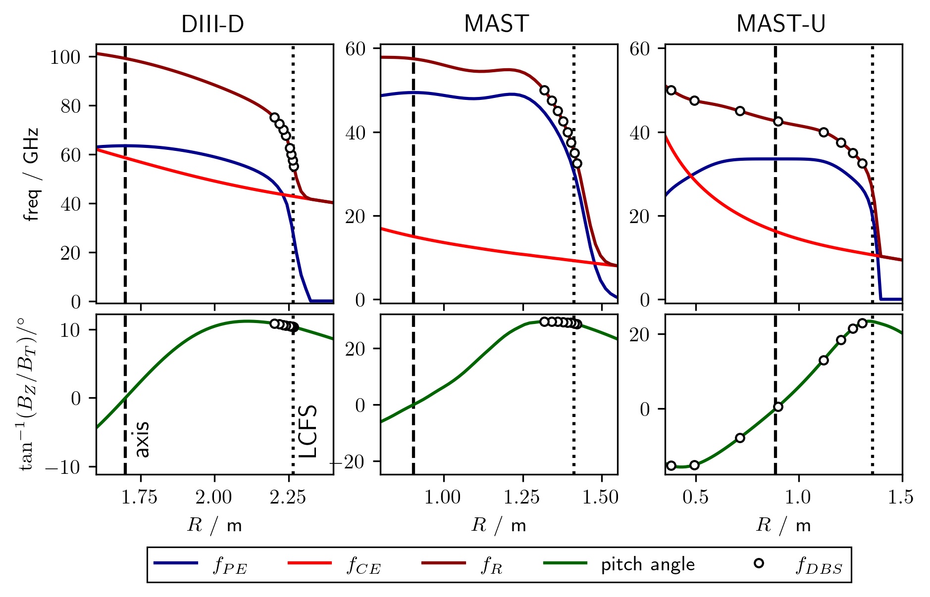
To investigate the effect of mismatch attenuation on the backscattered signal, the following methodology is typically [5, 18, 16, 12] used. Shots are repeated with as similar properties as possible: shape, density, plasma current, and heating. As such, the equilibrium properties are expected to be the same (within margins of error), likewise for the statistical properties of turbulence. The DBS is then steered toroidally for each shot. The poloidal launch angle is fixed and the toroidal launch angle varied. Hence, the probe beams reach similar radial locations and backscatter off similar perpendicular turbulent wavenumbers, but at different mismatch angles, as shown in Figure 2. The effect of mismatch angle on the signal is thereby ostensibly isolated from the various other complicated effects. In DIII-D, the mismatch angle at the cut-off location varies approximately linearly with toroidal launch angle. However, in MAST and MAST-U, the dependence of $\theta_{m}$ at the cut-off on the toroidal launch angle is non-trivial. Hence, although one optimizes the toroidal launch angle in experiments, one should remember that the physics actually depends on the mismatch angle, which is indirectly controlled by the toroidal launch angle.

For each of the three tokamaks (DIII-D, MAST, MAST-U), we study a series of repeated shots with the methodology outlined in the preceding paragraph. Since these tokamaks support a wide range of plasma equilibria, the shots studied in this paper are meant to be illustrative and not definitively representative of all possible plasma configurations. The experimental profiles are shown in Figure (4); more detail is available in other papers on DIII-D [16], MAST [5], and MAST-U [19].

Refer to caption — Figure 4: Here $f_{PE}$ is the plasma frequency, $f_{CE}$ is the cyclotron frequency, $f_{R}$ is the X-mode cut-off frequency, $\tan^{-1}(B_{Z}/B_{T})$ is the pitch angle, $B_{Z}$ is a poloidal component of the magnetic field, and $B_{T}$ the toroidal component. These values of these quantities on the midplane are plotted as a function of radius, $R$ . The DBS probe frequencies for DIII-D [7] (left), MAST [5] (middle), and MAST-U (UCLA system) (right) [19] are plotted as circles. DIII-D equilibrium data from shot 188839 at 1900 ms, MAST data from shot 29908 at 190 ms, and MAST-U data from shot 45290. All DBS systems were in X-mode for these shots.

III Cross-system study of mismatch attenuation

Using the methodology described in subsection II.2, we evaluate the effectiveness of the beam model in quantitatively account for mismatch in DIII-D, MAST, and MAST-U. The results are then compared with one another.

III.1 DIII-D

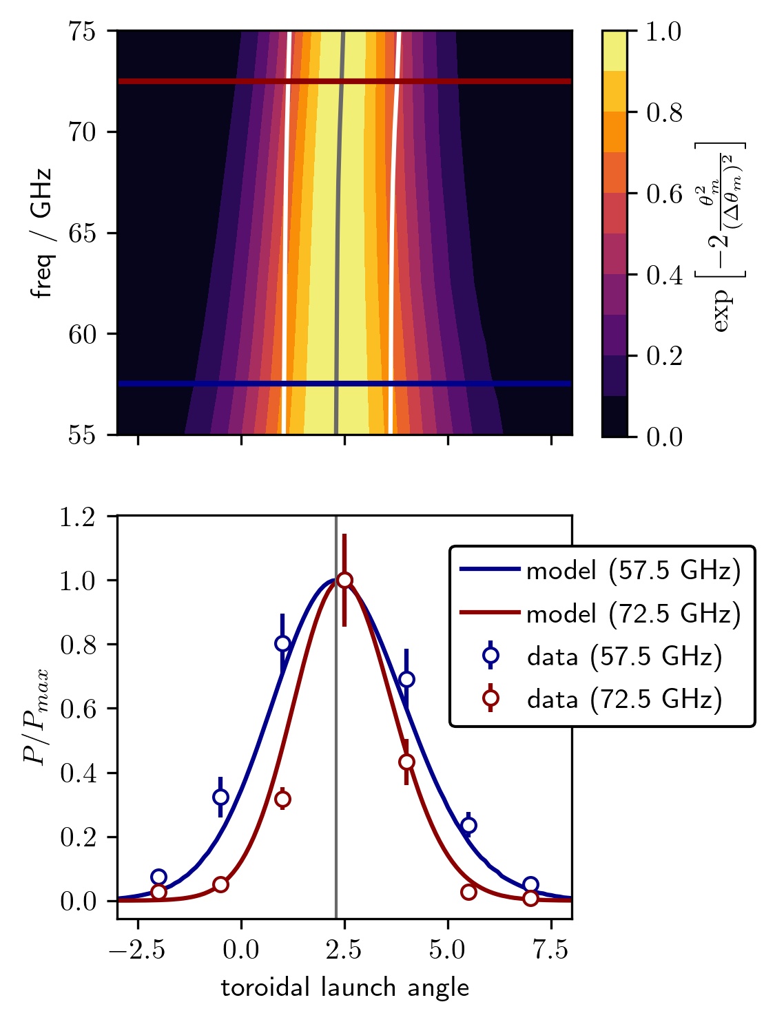
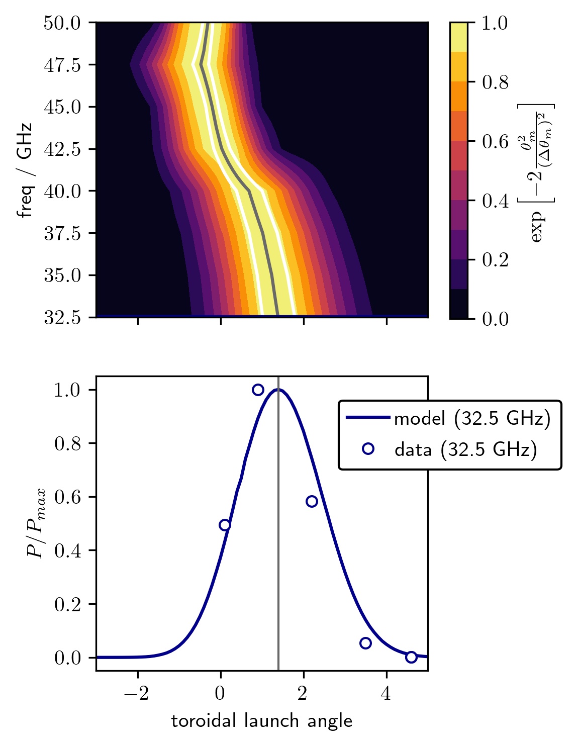
A new DBS system [7] was installed on the DIII-D tokamak in 2018. This system is capable of 2D steering of the probe beam; the poloidal and toroidal launch angles can both be independently varied. Toroidal sweeps at fixed poloidal angle were carried out on DIII-D using this DBS system [7, 16] to investigate the mismatch attenuation. The beam model predicts that mismatch tolerance decreases with increasing wavenumber, Figure 5 (top). This prediction is validated by experimental data, Figure 5 (bottom).

In DBS measurements, one typically attempts to minimise mismatch across all channels [5, 20], hopefully achieving reasonable signals across all channels. For the shots studied on DIII-D, the toroidal launch angles to achieve zero mismatch for all channels is very similarly, $2.4\pm 0.1^{\circ}$ , Figure 5. Hence, it is possible to achieve near-zero mismatch on all channels with an appropriate launch angle [16]. This is likely a consequence of the magnetic pitch angle not varying significantly over the different radial locations that the various channels reach. However, the equilibrium properties change with time; there may be good matching at certain times during the shot, but accounting for mismatch becomes important if one is interested in various times in a shot where the equilibrium properties are sufficiently different.

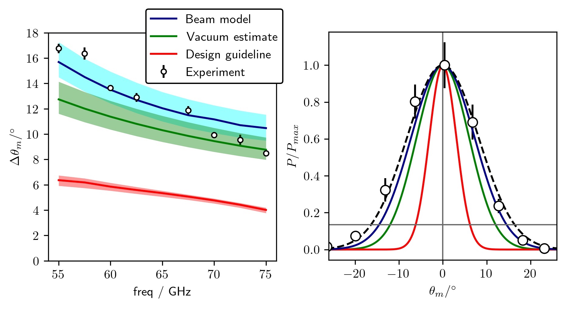
We proceed to quantitatively assess the beam model’s ability to account for mismatch attenuation, $\Delta\theta_{m}$ . We calculated $\Delta\theta_{m}$ with two different methods. Semi-analytically, by using equilibrium data, beam tracing with the Scotty code, and equation 4. Empirically, by fitting a Gaussian to the backscattered power as a function of toroidal launch angle (black dotted line, Figure 6 right). The difference in mismatch tolerance as calculated by Scotty and fitting of experimental data, appears to be quite large, up to $2^{\circ}$ , Figure 6 (left, difference between points and blue line). However, as we see from Figure 6 (right), a small difference in mismatch tolerance does not make a significant visual difference in the plots of power versus mismatch angle. We varied the launch widths of every frequency by $\pm 10\%$ , and find that this does indeed mostly account for the spread of mismatch tolerance. We also varied the launch beam curvature by $\pm 10\%$ , but the effect was much less pronounced. Changes in the smoothing schemes of the experimental equilibria resulted in changes to $\Delta\theta_{m}$ of around $0.5^{\circ}$ . It is likely that equilibrium reconstruction might also play a significant role, but we do not examine this in this paper.

Having shown that the beam model can indeed satisfactorily account for mismatch tolerance on DIII-D, we now evaluate other methods of finding the mismatch tolerance. The beam model requires the probe beam’s width and curvature as calculated from a beam tracing code. However, beam tracing codes are not yet widely implemented. On the other hand, ray tracing codes are widely available; they can be used to estimate the mismatch attenuation as follows. The wavenumber in equation (26) is calculated with ray tracing, the beam widths and curvatures are estimated with vacuum propagation, and then magnetic field’s shear and curvature are ignored. For the shots studied, this does indeed provide a rough estimate, Figure 6 (green line). We see that the earlier estimates for conservative design guidelines is indeed stricter than our estimate, Figure 6 (red line). Now that we have a quantitative model for mismatch, this design constraint may be somewhat relaxed.

III.2 MAST

The beam model was previously applied to MAST plasmas [12] for a single frequency, 55 GHz, and at a single time, 190 ms. In this work, we analyse the mismatch tolerance of all eight Q-band channels at 190ms, Figure 7. As with DIII-D, the mismatch tolerance in MAST is calculated in four different ways: by curve fitting a Gaussian to experimental data, with the full beam model, equation (4), with the plasma wavenumber but beam properties as estimated by vacuum propagation, equation (26), and with pre-beam-model estimate, equation (27) . The launch beam widths in Scotty were varied by $10\%$ to account for possible errors in their measurement. A systematic error of $3^{\circ}$ in the steering mirror’s rotation angle was used for calculating the experimental points, similar to previous work studying mismatch in MAST [5].

There are a few noteworthy points. First, that while Scotty’s agreement with experimental data in MAST is decent, Figure 7, it is noticeably worse than that of DIII-D, Figure 6 (right). This is possibly due to there being fewer points in the toroidal scan, leading to larger errors. Moreover, the wavenumber at the cut-off varies more strongly with toroidal launch angle for the MAST shots studied than DIII-D, which means the other pieces of the instrumentation weighting function could play a part. Secondly, vacuum propagation poorly estimates the beam’s properties and thus the mismatch tolerance, Figure 7 (green line). For reasons that are not entirely clear, the evolution of the beam is significantly more complicated in MAST than DIII-D. In such a situation, using beam tracing is vital.

III.3 MAST-U

There are two DBS systems installed on MAST-U, one from the University of California Los Angeles (UCLA) [21, 19] and the other from the Southwestern Institute of Physics (SWIP) [22, 23]; detailed information about these two systems are available in the cited references. The UCLA system operates in the Q-band and was already installed during MAST-U’s first campaign. The SWIP system has two bands, Q and V, and will be installed in time for the second campaign, which has yet to occur at the time of writing. Moreover, its exact quasioptical system might still be modified before installation. As such, the SWIP DBS is not evaluated in this work.

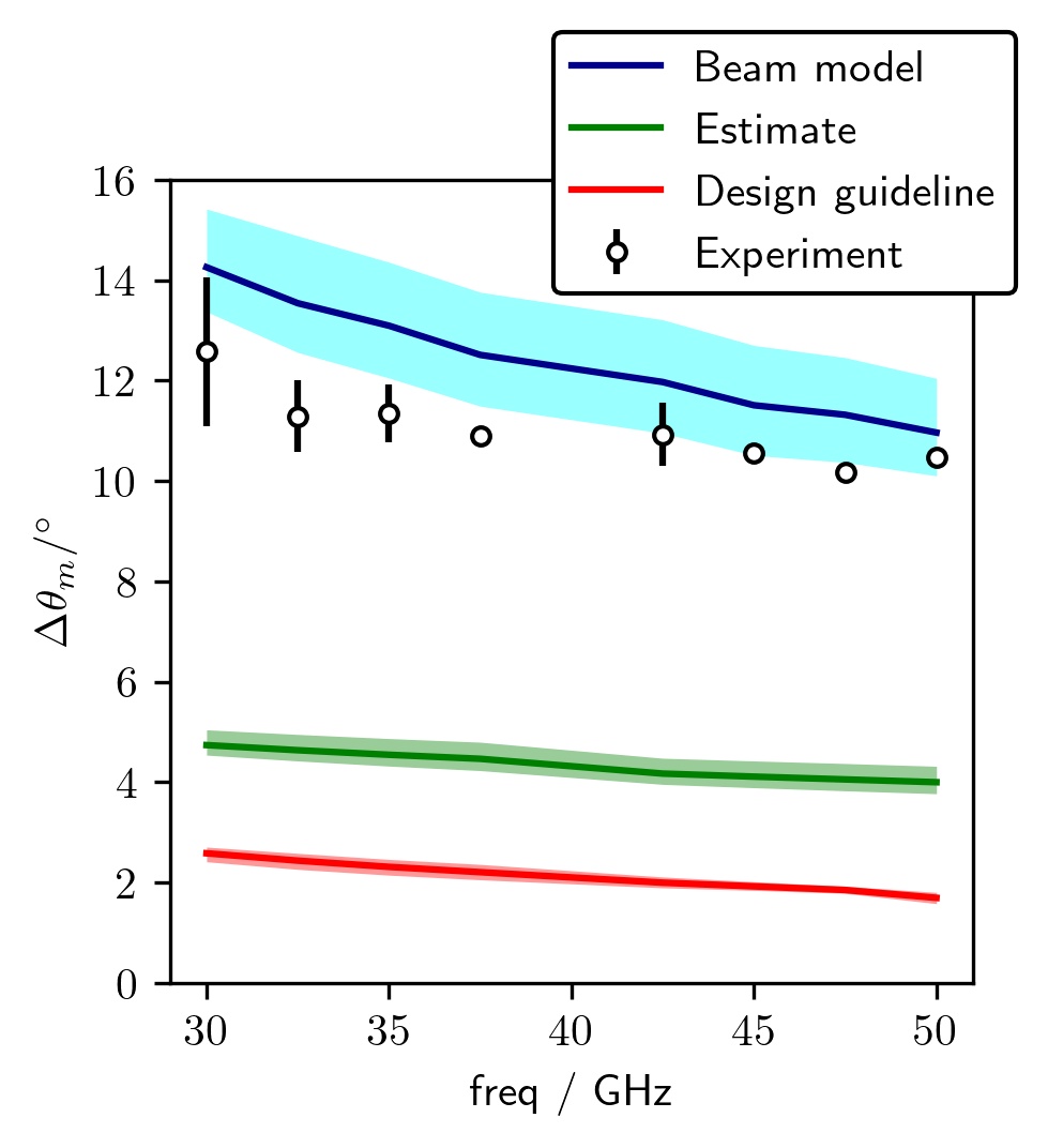
Preliminary results from MAST-U indicate decent agreement between the predicted and measured mismatch tolerances at low frequencies, Figure 8 (bottom). Since the Q-band frequencies reach significantly different locations with different pitch angles, see Figure 4, it is difficult to optimise the toroidal angle for low mismatch across all frequencies simultaneously, Figure 8 (top). Specifically, for these shots, the channels’ measurements span the outboard to the inboard, a dramatic range of locations. This is in contrast with DIII-D shot 188839, Figure 5, where all the frequencies reach the cut-off at significantly more similar locations. The situation is made more complicated by the probe beam’s wavevector changing directions during propagation and not generally being aligned with the group velocity, which makes beam’s wavevector’s direction relative to the magnetic field at the cut-off non-trivial.

At higher frequencies, the optimal toroidal launch angle is significantly smaller, Figure 8 (top). As such, there was no clear peak of backscattered power when the toroidal launch angle was varied in the experiments. At least one more point at a negative toroidal launch angle would have been required. Hence, we do not present a systematic comparison of theory and experiment for all frequencies, unlike MAST and DIII-D. The strong dependence of optimal launch angle on frequency poses another challenge: it is difficult to simultaneously optimise mismatch across all channels at once without repeating shots, making the beam model’s ability to quantitatively account for mismatch attenuation crucial for interpreting the measured data.

IV Optimizing mismatch tolerance

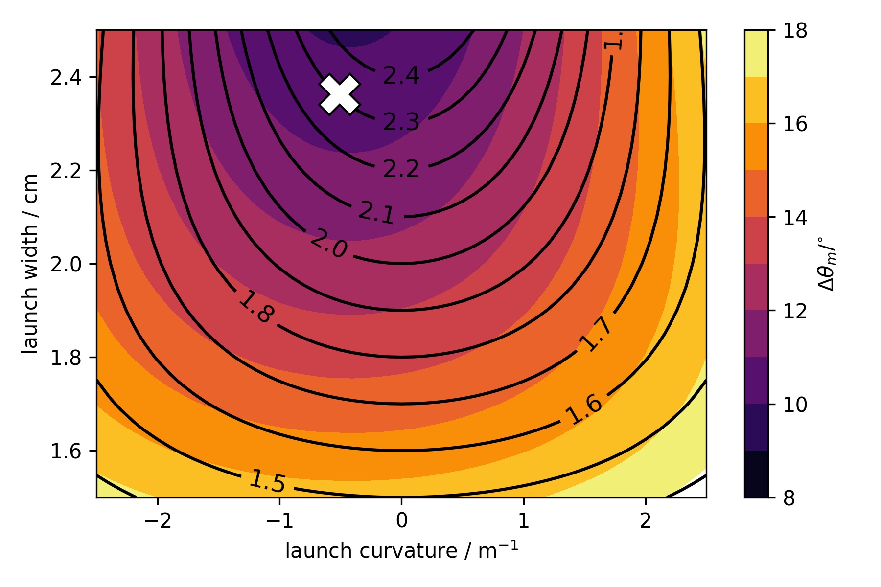
Now that we have established the beam model of DBS as a reliable quantitative method of determining the mismatch attenuation, we can leverage its insights to help us design new DBS systems with more tolerance to mismatch. This is complicated because such optimisation depends on the tokamak and what one is trying to measure. We present preliminary simulations for optimisation in this paper. We consider the DBS on DIII-D and try to see if we can increase the mismatch tolerance by adjusting the launch beam’s width and curvature, Figure 9. The plasma’s effect on the beam’s width and curvature plays a significant role in this optimisation, as seen from the difference between the black and filled contours. Note that in our simulations, the beam is launched from the steering optics: the steering mirror for DIII-D and the movable lens for MAST-U. The beam’s initial properties are specified at these locations, and not at plasma entry.

Our simulation results show that the mismatch tolerance can be significantly increased. For the particular case studied, this is achieved by having a smaller width as well as a low curvature at launch. It is possible that the parameter space accessible by quasioptical systems is limited, but such analysis is beyond the scope of this paper. Nonetheless, such analysis is likely important when designing new DBS systems, especially when pitch angle at the cut-off varies significantly across the probe frequencies.

V Discussion

The beam model is capable of calculating various contributions to the instrumentation weighting function, $F(l)$ . In this work, we evaluate one piece of this function: mismatch attenuation and the associated mismatch tolerance. We see that this approach appears to be more successful at explaining the toroidal scan results from DIII-D than MAST. It is possible that the other pieces of the weighting function [12] play a significant role in MAST’s toroidal scan’s results. This will be evaluated in a future paper.

Even though using beam tracing and the reciprocity theorem allows one to quantitatively calculate the mismatch attenuation, attempting to get good matching in experiments via prudent toroidal steering is still important for several reasons. First, the signal is larger, which makes it easier to analyse the data. Secondly, as we have seen in this paper, calculating the attenuation has some uncertainty involved, and thus having to correct for it might increase the uncertainty in the measured backscattered power.

VI Conclusions

In this paper, we have shown that the mismatch attenuation in conventional and spherical tokamaks can be quantitatively predicted by using beam tracing and reciprocity theorem. These predictions are validated with experiments on DIII-D, MAST, and MAST-U. Furthermore, we show that the beam model gives significantly better predictions of mismatch tolerance than previous estimates.

Being able to account for mismatch attenuation increases the versatility of DBS. However, preliminary analysis of MAST-U shows that attempting to get good matching over all channels simultaneously might prove challenging in certain cases, namely, when the pitch angle at the cut-off is significantly different for the various DBS channels. To address this issue, future DBS systems could be designed to have higher mismatch tolerances.

Acknowledgements.

This work was partly supported by the U.S. Department of Energy under contract numbers DE-AC02-09CH11466, DE-SC0019005, DE-SC0019352, DE-SC0020649, and DE-SC0019007. The United States Government retains a non-exclusive, paid-up, irrevocable, world-wide license to publish or reproduce the published form of this manuscript, or allow others to do so, for United States Government purposes. This work has been part-funded by the EPSRC Energy Programme [grant numbers EP/W006839/1 and EP/R034737/1]. To obtain further information on the data and models underlying this paper please contact PublicationsManager@ukaea.uk.

References

Hirsch et al. [2001] M. Hirsch, E. Holzhauer, J. Baldzuhn, B. Kurzan, and B. Scott, “Doppler reflectometry for the investigation of propagating density perturbations,” Plasma Physics and Controlled Fusion 43, 1641–1660 (2001).
Pratt et al. [2022] Q. Pratt, T. L. Rhodes, C. Chrystal, and T. A. Carter, “Comparison of doppler back-scattering and charge exchange measurements of e $\times$ b plasma rotation in the diii-d tokamak under varying torque conditions,” Plasma Physics and Controlled Fusion (2022).
Ruiz Ruiz et al. [ress] J. Ruiz Ruiz, F. I. Parra, V. H. Hall-Chen, N. Christen, B. Barnes, J. Candy, J. Garcia, C. Giroud, W. Guttenfelder, J. C. Hillesheim, C. Holland, N. T. Howard, Y. Ren, A. E. White, and . JET contributors, “Interpreting radial correlation doppler reflectometry using gyrokinetic simulations,” Plasma Physics and Controlled Fusion (In press).
Hennequin et al. [2004] P. Hennequin, C. Honoré, A. Truc, A. Quéméneur, N. Lemoine, J.-M. Chareau, and R. Sabot, “Doppler backscattering system for measuring fluctuations and their perpendicular velocity on tore supra,” Review of Scientific Instruments 75, 3881–3883 (2004).
Hillesheim et al. [2015] J. Hillesheim, N. Crocker, W. Peebles, H. Meyer, A. Meakins, A. Field, D. Dunai, M. Carr, N. Hawkes, M. Team, et al., “Doppler backscattering for spherical tokamaks and measurement of high-k density fluctuation wavenumber spectrum in mast,” Nuclear Fusion 55, 073024 (2015).
Shi et al. [2016] Z. Shi, W. Zhong, M. Jiang, Z. Yang, B. Zhang, P. Shi, W. Chen, J. Wen, C. Chen, B. Fu, et al., “A novel multi-channel quadrature doppler backward scattering reflectometer on the hl-2a tokamak,” Review of Scientific Instruments 87, 113501 (2016).
Rhodes et al. [2018] T. Rhodes, R. Lantsov, G. Wang, R. Ellis, and W. Peebles, “Optimized quasi-optical cross-polarization scattering system for the measurement of magnetic turbulence on the diii-d tokamak,” Review of Scientific Instruments 89, 10H107 (2018).
Happel et al. [2009] T. Happel, T. Estrada, E. Blanco, V. Tribaldos, A. Cappa, and A. Bustos, “Doppler reflectometer system in the stellarator tj-ii,” Review of Scientific Instruments 80, 073502 (2009).
Tokuzawa et al. [2021] T. Tokuzawa, K. Tanaka, T. Tsujimura, S. Kubo, M. Emoto, S. Inagaki, K. Ida, M. Yoshinuma, K. Watanabe, H. Tsuchiya, et al., “W-band millimeter-wave back-scattering system for high wavenumber turbulence measurements in lhd,” Review of Scientific Instruments 92, 043536 (2021).
Gusakov and Surkov [2004] E. Gusakov and A. Surkov, “Spatial and wavenumber resolution of doppler reflectometry,” Plasma physics and controlled fusion 46, 1143 (2004).
Bulanin and Yafanov [2006] V. V. Bulanin and M. V. Yafanov, “Spatial and spectral resolution of the plasma doppler reflectometry,” Plasma Physics Reports 32, 47–55 (2006).
Hall-Chen, Parra, and Hillesheim [2022] V. H. Hall-Chen, F. I. Parra, and J. C. Hillesheim, “Beam model of doppler backscattering,” Plasma Physics and Controlled Fusion 64, 095002 (2022).
Pereverzev [1996] G. Pereverzev, “Paraxial wkb solution of a scalar wave equation,” in Reviews of Plasma Physics: Volume 19, edited by B. Kadomtsev (Springer, 1996) pp. 1–48.
Poli, Peeters, and Pereverzev [2001] E. Poli, A. Peeters, and G. Pereverzev, “Torbeam, a beam tracing code for electron-cyclotron waves in tokamak plasmas,” Computer Physics Communications 136, 90–104 (2001).
Piliya and Popov [2002] A. Piliya and A. Y. Popov, “On application of the reciprocity theorem to calculation of a microwave radiation signal in inhomogeneous hot magnetized plasmas,” Plasma Physics and Controlled Fusion 44, 467 (2002).
Damba et al. [2022] J. Damba, Q. T. Pratt, V. H. Hall-Chen, R. Hong, and T. L. Rhodes, “Evaluation of the upgraded diii-d doppler backscattering system for high-wavenumber measurement and signal enhancement,” Submitted to Review of Scientific Instruments (2022).
Slusher and Surko [1980] R. Slusher and C. M. Surko, “Study of density fluctuations in plasmas by small-angle co2 laser scattering,” The Physics of Fluids 23, 472–490 (1980).
Damba et al. [2021] J. Damba, R. Hong, Q. Pratt, and T. Rhodes, “Toroidal matching of dbs for higher wavenumber measurement and signal enhancement during turbulence measurement in diii-d tokamak plasmas,” Bulletin of the American Physical Society (2021).
Rhodes et al. [2022] T. Rhodes, C. Michael, P. Shi, R. Scannell, S. Storment, Q. Pratt, R. Lantsov, V. H. Hall-Chen, N. Crocker, and W. Peebles, “Design elements and first data from a new doppler backscattering system on the mast-u spherical tokamak,” Submitted to Review of Scientific Instruments (2022).
Carralero et al. [2021] D. Carralero, T. Happel, T. Estrada, T. Tokuzawa, J. Martínez, E. de la Luna, A. Cappa, and J. García, “A feasibility study for a doppler reflectometer system in the jt-60sa tokamak,” Fusion Engineering and Design 173, 112803 (2021).
Storment et al. [2021] S. Storment, R. Scannell, P. Shi, C. Michael, Q. Pratt, T. Carter, and T. Rhodes, “A new combined doppler backscattering and cross-polarization scattering system for measurement of density and magnetic turbulence in the mast-u spherical tokamak,” Bulletin of the American Physical Society (2021).
Shi et al. [2019] Z. B. Shi, J. Wen, B. Wang, Z. C. Yang, W. L. Zhong, J. C. Hillesheim, S. Freethy, M. Jiang, P. W. Shi, K. R. Fang, Z. T. Liu, and M. Xu, “Development of quasi-optical system for the doppler backscattering reflectometers on the mast-u,” Proceedings of the 14th International Reflectometry Workshop for Fusion Plasma Diagnostics (2019).
Wen et al. [2021] J. Wen, Z. Shi, W. Zhong, Z. Yang, Z. Yang, B. Wang, M. Jiang, P. Shi, J. Hillesheim, S. Freethy, et al., “A remote gain controlled and polarization angle tunable doppler backward scattering reflectometer,” Review of Scientific Instruments 92, 063513 (2021).