Variable selection in
seemingly unrelated regressions
with random predictors
Abstract
This paper considers linear model selection when the response is vector-valued and the predictors are randomly observed. We propose a new approach that decouples statistical inference from the selection step in a “post-inference model summarization” strategy. We study the impact of predictor uncertainty on the model selection procedure. The method is demonstrated through an application to asset pricing.
, and
1 Introduction and overview
This paper develops a method for parsimoniously summarizing the shared dependence of many individual response variables upon a common set of predictor variables drawn at random. The focus is on multivariate Gaussian linear models where an analyst wants to find, among available predictors , a subset which work well for predicting response variables . The multivariate normal linear model assumes that a set of responses are linearly related to a shared set of covariates via
| (1) |
where is a non-diagonal covariance matrix.
Bayesian variable selection in (single-response) linear models is the subject of a vast literature, from prior specification on parameters (Bayarri et al., 2012) and models (Scott and Berger, 2006) to efficient search strategies over the model space (George and McCulloch, 1993; Hans, Dobra and West, 2007). For a more complete set of references we refer the reader to the reviews of Clyde and George (2004) and Hahn and Carvalho (2015). By comparison, variable selection has not been widely studied in concurrent regression models, perhaps because it is natural simply to apply existing variable selection methods to each univariate regression individually. Indeed, such joint regression models go by the name “seemingly unrelated regressions” (SUR) in the Bayesian econometrics literature, reflecting the fact that the regression coefficients from each of the separate regressions can be obtained in isolation from one another (i.e., conducting estimation as if were diagonal). However, allowing non-diagonal can lead to more efficient estimation (Zellner, 1962) and can similarly impact variable selection (Brown, Vannucci and Fearn, 1998; Wang, 2010).
This paper differs from Brown, Vannucci and Fearn (1998) and Wang (2010) in that we focus on the case where the predictor variables (the regressors, or covariates) are treated as random as opposed to fixed.Our goal will be to summarize codependence among multiple responses in subsequent periods, making the uncertainty in future realizations highly central to our selection objective. This approach is natural in many contexts (e.g., macroeconomic models) where the purpose of selection is inherently forward-looking. To our knowledge, no existing variable selection methods are suitable in this context. The new approach is based on the sparse summary perspective outlined in Hahn and Carvalho (2015), which applies Bayesian decision theory to summarize complex posterior distributions. By using a utility function that explicitly rewards sparse summaries, a high dimensional posterior distribution is collapsed into a more interpretable sequence of sparse point summaries.
A related approach to variable selection in multivariate Gaussian models is the Gaussian graphical model framework (Jones et al., 2005; Dobra et al., 2004; Wang and West, 2009). In that approach, the full conditional distributions are represented in terms of a sparse -by- precision matrix. By contrast, we partition the model into response and predictor variable blocks, leading to a distinct selection criterion that narrowly considers the -by- covariance between to .
1.1 Methods overview
Posterior summary variable selection consists of three phases: model specification and fitting, utility specification, and graphical summary. Each of these steps is outlined below. Additional details of the implementation are described in Section 2 and the Appendix.
Step 1: Model specification and fitting
The statistical model may be described compositionally as . For , the regression model (1) implies has the following block structure:
| (4) |
We denote the unknown parameters for the full joint model as where and .
For a given prior choice , posterior samples of all model parameters are computed by routine Monte Carlo methods, primarily Gibbs sampling. Details of the specific modeling choices and associated posterior sampling strategies are described in the Appendix.
A notable feature of our approach is that steps 2 (and 3) will be unaffected by modeling choices made in step 1 except insofar as they lead to different posterior distributions . In short, step 1 is “obtain a posterior distribution”; posterior samples then become inputs to step 2.
Step 2: Utility specification
For our utility function we use the log-density of the regression above. It is convenient to work in terms of negative utility, or loss:
| (5) |
where . Note that this log-density is being used in a descriptive capacity, not an inferential one; that is, all posterior inferences are based on the posterior distribution from step 1. The “action” is regarded as a point estimate of the regression parameters , which would be a good fit to future data drawn from the same model as the observed data.
Taking expectations over the posterior distribution of all unknowns
| (6) |
yields expected loss
| (7) |
where , , and , the overlines denote posterior means, and the final term is a constant with respect to .
Finally, we add an explicit penalty, reflecting our preference for sparse summaries:
| (8) |
where counts the number of non-zero elements in . In practice, we will use an approximation to this utility based on the penalty; optimal actions under this approximation will still be sparse.
Step 3: Graphical summary
Traditional applications of Bayesian decision theory derive point-estimates by minimizing expected loss for certain loss functions. The present goal is not an estimator per se, but a parsimonious summary of information contained in a complicated, high dimensional posterior distribution. This distinction is worth emphasizing because we have not one, but rather a continuum of loss functions, indexed by the penalty parameter . This class of loss functions can be used to organize the posterior distribution as follows.
Using available convex optimization techniques, expression (8) can be optimized efficiently for a range of values simultaneously. Posterior graphical summaries consist of two components. First, graphs depicting which response variables have non-zero coefficients on which predictor variables can be produced for any given . Second, posterior distributions of the quantity
| (9) |
can be used to gauge the impact has on the descriptive capacity of . Here, is the unpenalized optimal solution to the minimization of loss (8).
2 Posterior summary variable selection
The statistical model is given in equations (1) and (4); prior specification and model fitting details can be found in the Appendix. Alternatively, the models described in Brown, Vannucci and Fearn (1998) or Wang (2010) could be used. In this section, we flesh out the details of steps 2 and 3, which represent the main contributions of this paper.
2.1 Deriving the sparsifying expected utility function
Define the optimal posterior summary as the minimizing some expected loss . Here, the expectation is taken over the joint posterior predictive and posterior distribution: .
As described in the previous section, our loss takes the form of a penalized log conditional distribution:
| (10) |
where , , and is the vectorization of the action matrix The first term of this loss measures the distance (weighted by the precision ) between the linear predictor and a future response . The second term promotes a sparse optimal summary, . The penalty parameter determines the relative importance of these two components. Expanding the quadratic form gives:
| (11) |
Integrating over (and dropping the constant) gives:
| (12) |
where
| (13) |
and the overlines denote posterior means. Define the Cholesky decompositions and . To make the optimization problem tractable we replace the norm with the norm, leading to an expression that can be formulated in the form of a standard penalized regression problem:
| (14) |
with covariates , “data” , and regression coefficients (see the Appendix for details). Accordingly, (14) can be optimized using existing software such as the lars R package of Efron et al. (2004) and still yield sparse solutions.
2.2 Sparsity-utility trade-off plots
Rather than attempting to determine an “optimal” value of , we advocate displaying plots that reflect the utility attenuation due to -induced sparsification. We define the “loss gap” between a -sparse solution, , and the optimal unpenalized (non-sparse, ) summary, as
| (15) |
As a function of , is itself a random variable which we can sample by obtaining posterior draws from . The posterior distribution(s) of (for various ) therefore reflects the deterioration in utility attributable to “sparsification”. Plotting these distributions as a function of allows one to visualize this trade-off. Specifically, is the (posterior) probability that the -sparse summary is no worse than the non-sparse summary. Using this framework, a useful heuristic for obtaining a single sparse summary is to report the sparsest model (associated with the highest ) such that is higher than some pre-determined threshold, ; we adopt this approach in our application section.
We propose summarizing the posterior distribution of via two types of plots. First, one can examine posterior means and credible intervals of for a sequence of models indexed by . Similarly, one can plot across the same sequence of models. Also, for a fixed value of , one can produce graphs where nodes represent predictor variables and response variables and an edge is drawn between nodes whenever the corresponding element of is non-zero. All three types of plots are exhibited in Section 3.
2.3 Relation to previous methods
Loss function (14) is similar in form to the univariate DSS (decoupled shrinkage and selection) strategy developed by Hahn and Carvalho (2015). Our approach generalizes Hahn and Carvalho (2015) by optimizing over the matrix rather than a single vector of regression coefficients, extending the sparse summary utility approach to seemingly unrelated regression models (Brown, Vannucci and Fearn, 1998; Wang, 2010).
Additionally, the present method considers random predictors, , whereas Hahn and Carvalho (2015) considered only a matrix of fixed design points. The impact of accounting for random predictors on the posterior summary variable selection procedure is examined in more detail in the application section.
An important difference between the sparse summary utility approach and previous approaches is in the role played by the posterior distribution. Many Bayesian variable importance metrics are based on the posterior distribution of an indicator variable that records if a given variable is non-zero (included in the model). The model we will use in our application utilizes such an indicator vector, which is called . For example, a widely-used model selection heuristic is to examine the “inclusion probability” of predictor , defined as the posterior mean of component . However, any approach based on the posterior mean of necessarily ignores information about the codependence between its elements, which can be substantial in cases of collinear predictors. Our method focuses instead on the expected log-density of future predictions, which synthesizes information from all parameters simultaneously in gauging how important they are in terms of future predictions.
3 Applications
In this section, the sparse posterior summary method is applied to a data set from the finance (asset pricing) literature. A key component of our analysis will be a comparison between the posterior summaries obtained when the predictors are drawn at random versus when they are assumed fixed.
The response variables are returns on 25 tradable portfolios and our predictor variables are returns on 10 other portfolios thought to be of theoretical importance. In the asset pricing literature Ross (1976), the response portfolios represent assets to be priced (so-called test assets) and the predictor portfolios represent distinct sources of variation (so-called risk factors). More specifically, the test assets represent trading strategies based on company size (total value of stock shares) and book-to-market (the ratio of the company’s accounting valuation to its size); see Fama and French (1992) and Fama and French (2015) for details. Roughly, these assets serve as a lower-dimensional proxy for the stock market. The risk factors are also portfolios, but ones which are thought to represent distinct sources of risk. What constitutes a distinct source of risk is widely debated, and many such factors have been proposed in the literature (Cochrane, 2011). We use monthly data from July 1963 through February 2015, obtained from Ken French’s website:
http://mba.tuck.dartmouth.edu/pages/faculty/ken.french/.
Our analysis investigates which subset of risk factors are most relevant (as defined by our utility function). As our initial candidates, we consider factors known in previous literature as: market, size, value, direct profitability, investment, momentum, short term reversal, long term reversal, betting against beta, and quality minus junk. Each factor is constructed by cross-sectionally sorting stocks by various characteristics of a company and forming linear combinations based on these sorts. For example, the value factor is constructed using the book-to-market ratio of a company. A high ratio indicates the company’s stock is a “value stock” while a low ratio leads to a “growth stock” assessment. Essentially, the value factor is a portfolio built by going long stocks with high book-to-market ratio and shorting stocks with low book-to-market ratio. For detailed definitions of the first five factors, see Fama and French (2015). In the figures to follow, each is labeled as, for example, “Size2 BM3,” to denote the portfolio buying stocks in the second quintile of size and the third quintile of book-to-market ratio.
Recent related work includes Ericsson and Karlsson (2004) and Harvey and Liu (2015). Ericsson and Karlsson (2004) follow a Bayesian model selection approach based off of inclusion probabilities, representing the preliminary inference step of our methodology. Harvey and Liu (2015) take a different approach that utilizes multiple hypothesis testing and bootstrapping.
3.1 Results
As described in Section 1.1, the first step of our analysis consists of fitting a Bayesian model. We fit model (1) using a variation of the well-known stochastic search variable selection algorithm of George and McCulloch (1993) and similar to Brown, Vannucci and Fearn (1998) and Wang (2010). Details are given in the Appendix.
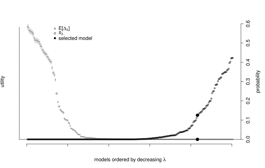
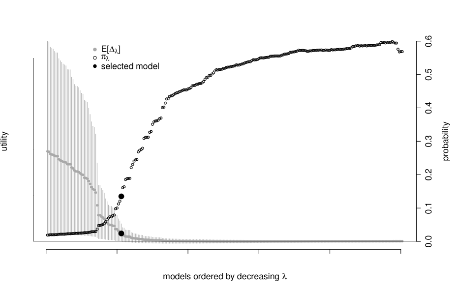
In the subsections to follow, we will show the following two figures. First, we plot the expectation of (and associated posterior credible interval) across a range of penalties. Recall, is the “loss gap” between a sparse summary and the best non-sparse (saturated) summary, meaning that smaller values are “better”. Additionally, we plot the probability that a given model is no worse than the saturated model on this same figure, where “no worse” means . Note that even for very weak penalties (small ), the distribution of will have non-zero variance and therefore even if it is centered about zero, some mass can be expected to fall above zero; practically, this means that is a very high score.
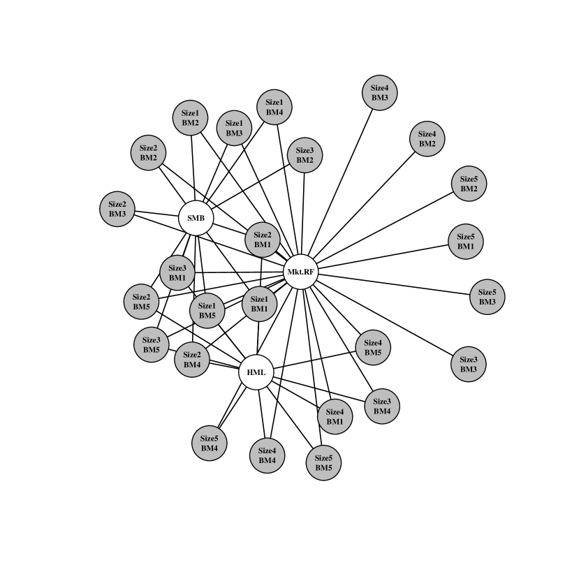
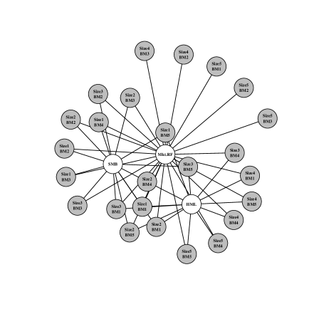
Second, we display a summary graph of the selected variables for the threshold. Recall that this is the highest penalty (sparsest graph) that is no worse than the saturated model with posterior probability. For these graphs, the response and predictor variables are colored gray and white, respectively. A test asset label of, for example, “Size2 BM3,” denotes the portfolio that buys stocks in the second quintile of size and the third quintile of book-to-market ratio. The predictors without connections to the responses under the optimal graph are not displayed.
These two figures are shown in four scenarios:
-
1.
Random predictors.
-
2.
Fixed predictors.
-
3.
Random predictors under alternative prior.
-
4.
Fixed predictors under alternative prior.
The “alternative prior” scenario serves to show the impact of the statistical modeling comprising step 1. Specifically, we use the same Monte Carlo model fitting procedure as before (described in the Appendix) but fix to the identity vector. That is, we omit the point-mass component of the priors for the elements of .
3.1.1 Random predictors
This section introduces our baseline example where the risk factors (predictors) are random. We evaluate the set of potential models by analyzing plots such as figure 2. This shows and evaluated across a range of values. Additionally, we display the posterior uncertainty in the metric with gray vertical uncertainty bands: these are the centered posterior credible intervals where . As the accuracy of the sparsified solution increases, the posterior of concentrates around zero by construction, and the probability of the model being no worse than the saturated model, , increases. We choose the sparsest model such that its corresponding . This model is displayed in figure 2 and is identified by the black dot in figure 2.
The selected set of factors in graph 2 are the market (Mkt.RF), value (HML), and size (SMB). This three factor model is no worse than the saturated model with posterior probability where all test assets are connected to all risk factors. Note also that in our selected model almost every test asset is distinctly tied to one of either value or size and the market factor. These are the three factors of Ken French and Eugene Fama’s pricing model developed in Fama and French (1992). They are known throughout the finance community as being “fundamental dimensions” of the financial market, and our procedure is consistent with this widely held belief at a small level.
The characteristics of the test assets in graph 2 are also important to highlight. The test portfolios that invest in small companies (“Size1” and “Size2”) are primarily connected to the SMB factor which is designed as a proxy for the risk of small companies. Similarly, the test portfolios that invest in high book-to-market companies (“BM4” and “BM5”) have connections to the HML factor which is built on the idea that companies whose book value exceeds the market’s perceived value should generate a distinct source of risk. As previously noted, all of the test portfolios are connected to the market factor suggesting that it is a relevant predictor even for the sparse selection criterion.
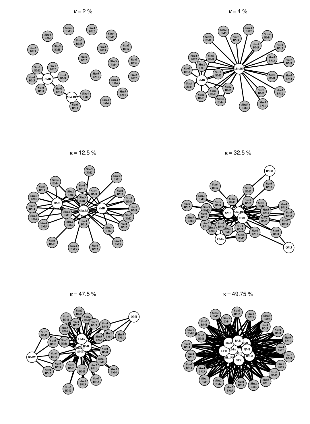
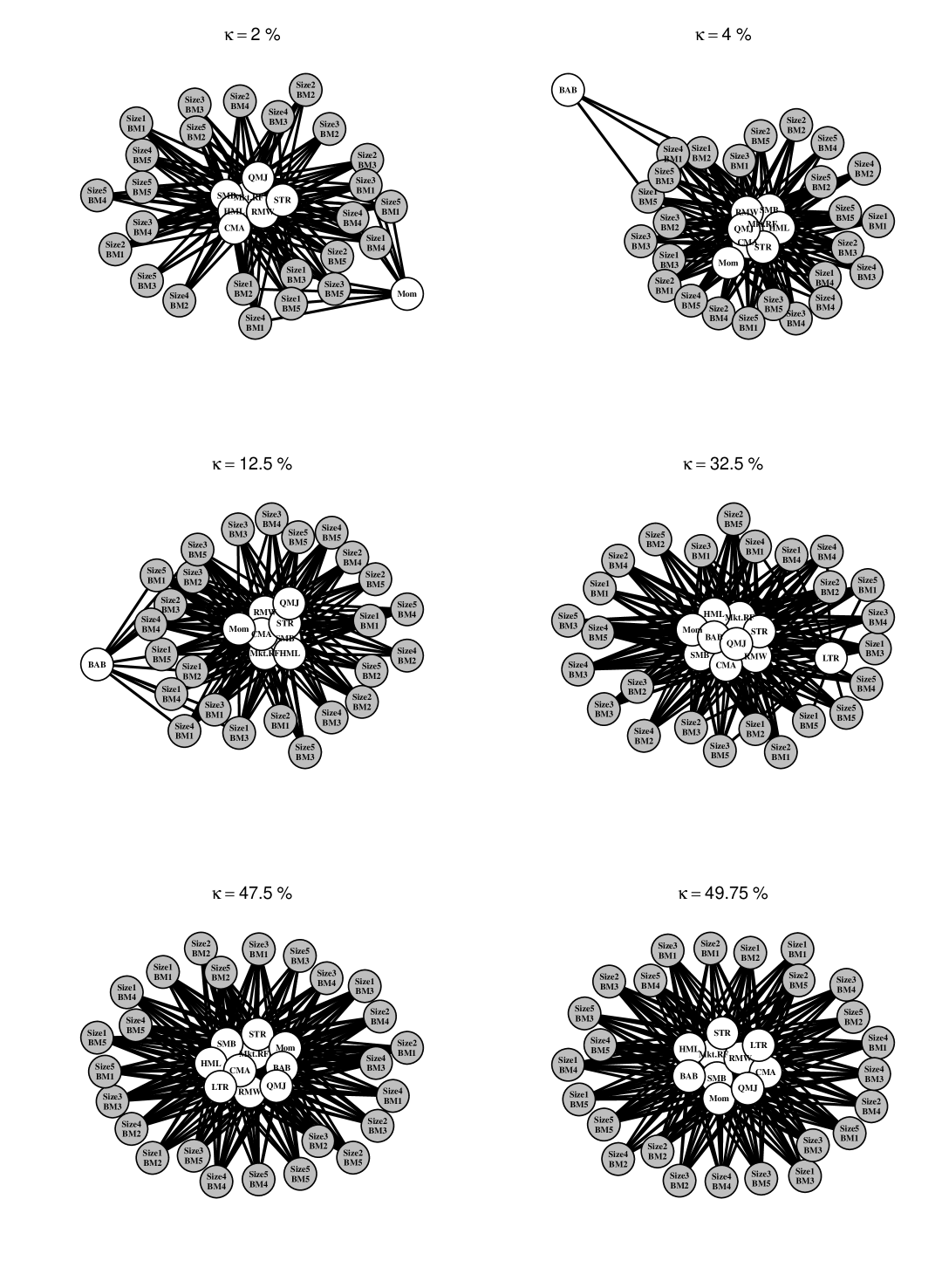
In figure 3, we examine how different choices of the threshold change the selected set of risk factors. In this analysis, there is a tradeoff between the posterior probability of being “close” to the saturated model and the utility’s preference for sparsity. When the threshold is low ( and %) the summarization procedure selects relatively sparse graphs with up to three factors (Mkt.RF, HML, and SMB). The market (Mkt.RF) and size (SMB) factors appear first, connected to a small number of the test assets (%). As the threshold is increased, the point summary becomes denser and correspondingly more predictively accurate (as measured by the utility function). The value factor (HML) enters at % and quality minus junk (QMJ), investment (CMA), and profitability (RMW) factors enter at %. The graph for % excluding QMJ is essentially the new five factor model proposed by Fama and French (2015). The five Fama-French factors (plus OMJ with three connections) persist up to the threshold. This indicates that, up to a high posterior probability, the five factor model of Fama and French (2015) does no worse than an asset pricing model with all ten factors connected to all test assets.
Notice also that our summarization procedure displays the specific relationship between the factors and test assets through the connections. Using this approach, the analyst is able to identify which predictors drive variation in which responses and at what thresholds they may be relevant. This feature is significant for summarization problems where individual characteristics of the test portfolios and their joint dependence on the risk factors is may be a priori unclear.
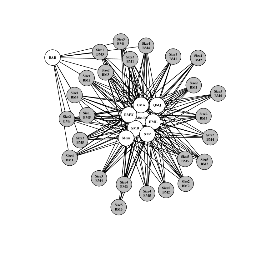
As approaches the threshold ( in figure 3), the model summary includes all ten factors. Requesting a summary with this level of certainty results in little sparsification. However, compared to the nearby model with only six factors, we also now know that the remaining four contribute little to our utility. These factors are betting against beta (BAB), momentum (Mom), long term reversal (LTR), and short term reversal (STR). Sparse posterior summarization applied in this context allows an analyst to study the impact of risk factors on pricing while taking uncertainty into account. Coming to a similar conclusion via common alternative techniques (e.g., component-wise ordinary least squares combined with thresholding by -statistics) is comparatively ad hoc; our method is simply a perspicuous summary of a posterior distribution. Likewise, applying sparse regression techniques based on penalized likelihood methods would not take into account the residual correlation , nor would that approach naturally accommodate random predictors.

3.1.2 Fixed predictors
In this section, we consider posterior summarization with the loss function derived under the assumption of fixed predictors. The analogous loss function when the predictor matrix is fixed is:
| (16) |
with , , and ; compare to (13) and (14). The derivation of (16) is similar to the presentation in Section 2 and may be found in the Appendix. The corresponding version of the loss gap is
| (17) |
which has distribution induced by the posterior over rather than as before. By fixing X, the posterior of has smaller dispersion which results in denser summaries for the same level of . For example, compare how dense Figure 5 is relative to Figure 2. The denser graph in Figure 5 contains nine out of ten potential risk factors compared to just three in Figure 2, which correspond to the Fama-French factors described in Fama and French (1992). Recall, both graphs represent the sparsest model such that the probability of being no worse than the saturated model is greater than — the difference is that one of the graphs defines “worse-than” in terms of a fixed set of risk factor returns while the other acknowledge that those returns are themselves uncertain in future periods.
Figure 6 demonstrates this problem for several choices of the uncertainty level. Regardless of the uncertainty level chosen, the selected models contain most of the ten factors and many edges. In fact, it is difficult to distinguish even the and models.
3.1.3 Alternative prior analysis
Here, we consider how our posterior summaries change as a function of using a different posterior, based on a different choice of prior. Specifically, in this section we do not employ model selection point-mass priors on the elements of as we did in the above analysis. These results are displayed in figures 8 and 8. Broadly, the same risk factors are flagged as important — the market factor followed by the size (SMB) and value (HML) factors. One notable difference is that the quality minus junk (QMJ), investment (CMA), and profitability (RMW) factors appear at smaller levels of . This result is intuitive in the sense that point-mass priors demand stronger evidence for a variable to impact the posterior means defining the loss function. Without the strong shrinkage imposed by the point-mass priors, these risk factors show up more strongly in the posterior and hence in the posterior summary. In each case, the three Fama and French factors from Fama and French (1992) predictably appear and seem to be the only relevant factors for pricing these 25 portfolios.
Similarly, the weaker shrinkage model in the fixed predictor version (figures 10 and 10) yields yet denser summaries (for a given level of ).


3.1.4 Comparison of four scenarios at fixed
The selected summary graphs for the four scenarios are displayed together for comparison in figure 11. Observe that graphs (c) and (d) selected under the alternative prior are marginally denser than their counterparts (a) and (b) under the point-mass model selection prior. However, the assumption of random predictors results in notably sparser summaries – graphs (a) and (c) are much sparser than (b) and (d). These comparisons emphasize the impact that incorporating random predictors may have on a variable selection procedure; especially the present approach where we extract point summaries from a posterior by utilizing uncertainty in all unknowns .


4 Conclusion
In this paper, we propose a general model selection procedure for multivariate linear models when future realizations of the predictors are unknown. Such models are widely used in many areas of science and economics, including genetics and asset pricing. Our utility-based sparse posterior summary procedure is a multivariate extension of the “decoupling shrinkage and selection” methodology of Hahn and Carvalho (2015). The approach we develop has three steps: (i) fit a Bayesian model, (ii) specify a utility function with a sparsity-inducing penalty term and optimize its expectation, and (iii) graphically summarize the posterior impact (in terms of utility) of the sparsity penalty. Our utility function is based on the kernel of the conditional distribution responses given the predictors and can be formulated as a tractable convex program. We demonstrate how our procedure may be used in asset pricing under a variety of modeling choices.
The remainder of this discussion takes a step back from the specifics of the seemingly unrelated regressions model and considers a broader role for utility-based posterior summaries.
A paradox of applied Bayesian analysis is that posterior distributions based on relatively intuitive models like the SUR model are often just as complicated as the data itself. For Bayesian analysis to become a routine tool for practical inquiry, methods for summarizing posterior distributions must be developed apace with the models themselves. A natural starting point for developing such methods is decision theory, which suggests developing loss functions specifically geared towards practical posterior summary. As a matter of practical data analysis, articulating an apt loss function has been sorely neglected relative to the effort typically lavished on the model specification stage, specifically prior specification. Ironically (but not surprisingly) our application demonstrates that one’s utility function has a dominant effect on the posterior summaries obtained relative to which prior distribution is used.
This paper makes two contributions to this area of “utility design”. First, we propose that the likelihood function has a role to play in posterior summary apart from its role in inference. That is, one of the great practical virtues of likelihood-based statistics is that the likelihood serves to summarize the data by way of the corresponding point estimates. By using the log-density as our utility function applied to future data, we revive the fundamental summarizing role of the likelihood. Additionally, note that this approach allows three distinct roles for parameters. First, all parameters of the model appear in defining the posterior predictive distribution. Second, some parameters appear in defining the loss function; plays this role in our analysis. Third, some parameters define the action space. In this framework there are no “nuisance” parameters that vanish from the estimator as soon as a marginal posterior is obtained. Once the likelihood-based utility is specified, it is a natural next step to consider augmenting the utility to enforce particular features of the desired point summary. For example, our analysis above was based on a utility that explicitly rewards sparsity of the resulting summary. A traditional instance of this idea is the definition of high posterior density regions, which are defined as the shortest, contiguous interval that contains a prescribed fraction of the posterior mass.
Our second contribution is to consider not just one, but a range, of utility functions and to examine the posterior distributions of the corresponding posterior loss. Specifically, we compare the utility of a sparsified summary to the utility of the optimal non-sparse summary. Interestingly, these utilities are random variables themselves (defined by the posterior distribution) and examining their distributions provides a fundamentally Bayesian way to measure the extent to which the sparsity preference is driving one’s conclusions. The idea of comparing a hypothetical continuum of decision-makers based on the posterior distribution of their respective utilities represents a principled Bayesian approach to exploratory data analysis. This is an area of ongoing research.
Appendix A Matrix-variate Stochastic Search
A.1 Model fitting: The marginal and conditional distributions
The future values of the response and covariates are unknown. Acknowledging this uncertainty is important in the overall decision of which covariates to select and is a necessary ingredient of the selection procedure. As our examples consider financial asset return data, we choose to model the marginal distribution of the covariates via a latent factor model detailed in Murray et al. (2013). The responses are modeled conditionally on the covariates via a matrix-variate stochastic search which is a multivariate of extension of stochastic search variable selection (SSVS) from George and McCulloch (1993). Recalling the block structure for the covariance of the full joint distribution of :
| (20) |
we obtain posterior samples of by sampling the conditional model parameters using a matrix-variate stochastic search algorithm (described below) and sampling the covariance of from a latent factor model where it is marginally normally distributed. To reiterate our procedure is
-
•
is sampled from independent latent factor model,
-
•
is sampled from matrix-variate MCMC,
-
•
is sampled from matrix-variate MCMC.
A.1.1 Modeling a full residual covariance matrix
In order to sample a full residual covariance matrix, we augment the predictor matrix with a latent factor by substituting :
| (21) |
where is now diagonal. Assuming that is shared among all response variables and is a vector of all coefficients , the total residual variance may be expressed as:
| (22) |
We incorporate this latent factor model into the matrix-variate MCMC via a simple Gibbs step to draw posterior samples of . This augmentation allows us to draw samples of that are not constrained to be diagonal.
A.1.2 Modeling the marginal distribution: A latent factor model
We model covariates via a latent factor model of the form:
| (23) |
where is assumed diagonal and the set of latent factors are independent. The covariance of the covariates is constrained by the factor decomposition and takes the form:
| (24) |
Recall that this is only a potential choice for the and it is chosen here primarily motivated by the applied context where financial assets tend to depend across each other through common factors. Our variable selection procedure would follow if any other choice was made at this point. To estimate this model, a convenient, efficient choice is the R package bfa (Murray, 2015). The software allows us to sample the marginal covariance as well as the marginal mean via a simple Gibbs step assuming a normal prior on .
A.1.3 Modeling the conditional distribution: A matrix-variate stochastic search
We model the conditional distribution, , by developing a multivariate extension of stochastic search variable selection of George and McCulloch (1993). Recall that the conditional model is: . In order to sample different subsets of covariates (different models) during the posterior simulations, we introduce an additional parameter that is a binary vector identifying a particular model. In other words, all entries for which denote covariate as included in model . Specifically, we write the model identified by as . As in George and McCulloch (1993), we aim to explore the posterior on the model space, . Our algorithm explores this model space by calculating a Bayes factor for a particular model . Given that the response Y is matrix instead of a vector, we derive the Bayes factor as a product of vector response Bayes factors. This is done by separating the marginal likelihood of the response matrix as a product of marginal likelihoods across the separate vector responses. This derivation requires our priors to be independent across the responses and is shown in the Appendix. It is important to note that we do not run a standard SSVS on each univariate response regression separately. Instead, we generalize George and McCulloch (1993) and require all covariates to be included or excluded from a model for each of the responses simultaneously.
The marginal likelihood requires priors for the parameters and parameters in our model. We choose the standard g-prior for linear models because it permits an analytical solution for the marginal likelihood integral (Zellner, 1986; Zellner and Siow, 1984; Liang et al., 2008a).
Our Gibbs sampling algorithm directly follows the stochastic search variable selection procedure described in George and McCulloch (1993) using these calculated Bayes factors, now adapted to a multivariate setting. The aim is to scan through all possible covariates and determine which ones to include in the model identified through the binary vector . At each substep of the MCMC, we consider an individual covariate within a specific model and compute its inclusion probability as a function of the model’s prior probability and the Bayes factors:
The Bayes factor is a ratio of marginal likelihoods for the model with covariate included and the null model, and is the analogous Bayes factor for the model without covariate . The prior on the model space, , can either be chosen to adjust for multiplicity or to be uniform - our results appear robust to both specifications. In this setting, adjusting for multiplicity amounts to putting equal prior mass on different sizes of models. In contrast, the uniform prior for models involving covariates puts higher probability mass on larger models, reaching a maximum for models with covariates included. The details of the priors on the model space and parameters, including an empirical Bayes choice of the g-prior hyperparameter, are discussed in the Appendix.
A.2 Details
Assume we have observed realizations of data . For model comparison, we calculate the Bayes factor with respect to the null model without any covariates. First, we calculate a marginal likelihood. This likelihood is obtained by integrating the full model over and multiplied by a prior, , for these parameters. A Bayes factor of a given model versus the null model, with:
| (25) |
We assume independence of the priors across columns of so we can write the integrand in (25) as a product across each individual response vector:
with:
| (26) |
Therefore, the Bayes factor for this matrix-variate model is just a product of Bayes factors for the individual multivariate normal models.
| (27) |
with:
| (28) |
The simplification of the marginal likelihood calculation is crucial for analytical simplicity and for the resulting SSVS algorithm to rely on techniques already developed for univariate response models. In order to calculate the integral for each Bayes factor, we need priors on the parameters and . Since the priors are independent across the columns of , we aim to define , which we express as the product: . Motivated by the work on regression problems of Zellner, Jeffreys, and Siow, we choose a non-informative prior for and the popular g-prior for the conditional prior on , (Zellner, 1986), (Zellner and Siow, 1980), (Zellner and Siow, 1984), (Jeffreys, 1961):
| (29) |
Under this prior, we have an analytical form for the Bayes factor:
| (30) | ||||
| (31) |
where and are the sum of squared errors from the linear regression of column on covariates and is the number of covariates in model . We allow the hyper parameter to vary across columns of and depend on the model, denoted by writing, .
We aim to explore the posterior of the model space, given our data:
| (32) |
where the denominator is a normalization factor. In the spirit of traditional stochastic search variable selection Garcia-Donato and Martinez-Beneito (2013), we propose the following Gibbs sampler to sample this posterior.
A.3 Gibbs Sampling Algorithm
Once the parameters and are integrated out, we know the form of the full conditional distributions for . We sample from these distributions as follows:
-
1.
Choose column and consider two models and such that:
-
2.
For each model, calculate and as defined by (30).
-
3.
Sample
where
Using this algorithm, we visit the most likely models given our set of responses. Under the model and prior specification, there are closed-form expressions for the posteriors of the model parameters and .
A.4 Hyper Parameter for the -prior
We use a local empirical Bayes to choose the hyper parameter for the -prior in (29). Since we allow to be a function of the columns of as well as the model defined by , we calculate a separate for each univariate Bayes factor in (29) above. An empirical Bayes estimate of maximizes the marginal likelihood and is constrained to be non-negative. From Liang et al. (2008b), we have:
| (33) | ||||
| (34) |
For univariate stochastic search, the literature recommends choosing a fixed as the number of data points Garcia-Donato and Martinez-Beneito (2013). However, the multivariate nature of our model induced by the vector-valued response makes this approach unreliable. Since each response has distinct statistical characteristics and correlations with the covariates, it is necessary to vary among different sampled models and responses. We find that this approach provides sufficiently stable estimation of the inclusion probabilities for the covariates.
Appendix B Derivation of lasso form
In this section of the Appendix, we derive the penalized objective (lasso) forms of the utility functions. After integration over , the utility takes the form (from equation (12)):
| (35) |
where , , and , and the overlines denote posterior means. Defining the Cholesky decompositions: and , combining the matrix traces, completing the square with respect to , and converting the trace to the vectorization operator, we obtain:
| (36) |
The proportionality in line 2 is up to an additive constant with respect to the action variable, . We arrive at the final utility by distributing the vectorization and rewriting the inner product as a squared norm.
| (37) |
The norm penalty yields a difficult combinatorial optimization problem even for a relatively small dimensions (). Thus, one may use an norm as the most straightforward approximation to the norm, yielding the loss function:
| (38) |
Appendix C Derivation of the loss function under fixed predictors
We devote this section to deriving an analogous loss function for multivariate regression when the predictors are assumed fixed. Notice that this is essentially an extension of Hahn and Carvalho (2015) to the multiple response case and adds to the works of Brown, Vannucci and Fearn (1998) and Wang (2010) by providing a posterior summary strategy that relies on more than just marginal quantities like posterior inclusion probabilities.
Suppose we observe realizations of the predictor vector defining the design matrix . Future realizations at this fixed set of predictors are generated from a matrix normal distribution:
| (39) |
In this case, the optimal posterior summary minimizes the expected loss . Here, the expectation is taken over the joint space of the predictive and posterior distributions: where is now absent since we are relegated to predicting at the observed covariate matrix X. We define the utility function using the negative kernel of distribution (39) where, as before, is the summary defining the sparsified linear predictor and :
| (40) |
Expanding the inner product and dropping terms that do not involve , we define the loss up to proportionality:
| (41) |
Analogous to the stochastic predictors derivation, we integrate over to obtain our expected loss:
| (42) |
where, similar to the random predictor case, , , , and the overlines denote posterior means. The subscript is used to denote quantities calculated at fixed design points X. Defining the Cholesky decompositions: and and replacing the norm with the norm, this expression can be formulated in the form of a standard penalized regression problem:
| (43) |
with covariates , “data” , and regression coefficients . Accordingly, (14) can be optimized using existing software such as the lars R package of Efron et al. (2004).
We use loss function (43) as a point of comparison to demonstrate how incorporating covariate uncertainty may impact the summarization procedure in our applications.
References
- Bayarri et al. (2012) {barticle}[author] \bauthor\bsnmBayarri, \bfnmM. J.\binitsM. J., \bauthor\bsnmBerger, \bfnmJ. O.\binitsJ. O., \bauthor\bsnmForte, \bfnmA.\binitsA. and \bauthor\bsnmGarcia-Donato, \bfnmG.\binitsG. (\byear2012). \btitleCriteria for Bayesian model choice with application to variable selection. \bjournalThe Annals of Statistics \bvolume40 \bpages1550–1577. \endbibitem
- Brown, Vannucci and Fearn (1998) {barticle}[author] \bauthor\bsnmBrown, \bfnmPhilip J\binitsP. J., \bauthor\bsnmVannucci, \bfnmMarina\binitsM. and \bauthor\bsnmFearn, \bfnmTom\binitsT. (\byear1998). \btitleMultivariate Bayesian variable selection and prediction. \bjournalJournal of the Royal Statistical Society: Series B (Statistical Methodology) \bvolume60 \bpages627–641. \endbibitem
- Clyde and George (2004) {barticle}[author] \bauthor\bsnmClyde, \bfnmM.\binitsM. and \bauthor\bsnmGeorge, \bfnmE. I.\binitsE. I. (\byear2004). \btitleModel uncertainty. \bjournalStatistical Science \bvolume19 \bpages81–94. \endbibitem
- Cochrane (2011) {barticle}[author] \bauthor\bsnmCochrane, \bfnmJohn H\binitsJ. H. (\byear2011). \btitlePresidential address: Discount rates. \bjournalThe Journal of Finance \bvolume66 \bpages1047–1108. \endbibitem
- Dobra et al. (2004) {barticle}[author] \bauthor\bsnmDobra, \bfnmAdrian\binitsA., \bauthor\bsnmHans, \bfnmChris\binitsC., \bauthor\bsnmJones, \bfnmBeatrix\binitsB., \bauthor\bsnmNevins, \bfnmJoseph R\binitsJ. R., \bauthor\bsnmYao, \bfnmGuang\binitsG. and \bauthor\bsnmWest, \bfnmMike\binitsM. (\byear2004). \btitleSparse graphical models for exploring gene expression data. \bjournalJournal of Multivariate Analysis \bvolume90 \bpages196–212. \endbibitem
- Efron et al. (2004) {barticle}[author] \bauthor\bsnmEfron, \bfnmBradley\binitsB., \bauthor\bsnmHastie, \bfnmTrevor\binitsT., \bauthor\bsnmJohnstone, \bfnmIain\binitsI., \bauthor\bsnmTibshirani, \bfnmRobert\binitsR. \betalet al. (\byear2004). \btitleLeast angle regression. \bjournalThe Annals of statistics \bvolume32 \bpages407–499. \endbibitem
- Ericsson and Karlsson (2004) {btechreport}[author] \bauthor\bsnmEricsson, \bfnmJohan\binitsJ. and \bauthor\bsnmKarlsson, \bfnmSune\binitsS. (\byear2004). \btitleChoosing Factors in a Multifactor Asset Pricing Model: A Bayesian Approach \btypeTechnical Report, \bpublisherStockholm School of Economics. \endbibitem
- Fama and French (1992) {barticle}[author] \bauthor\bsnmFama, \bfnmEugene F\binitsE. F. and \bauthor\bsnmFrench, \bfnmKenneth R\binitsK. R. (\byear1992). \btitleThe cross-section of expected stock returns. \bjournalthe Journal of Finance \bvolume47 \bpages427–465. \endbibitem
- Fama and French (2015) {barticle}[author] \bauthor\bsnmFama, \bfnmEugene F\binitsE. F. and \bauthor\bsnmFrench, \bfnmKenneth R\binitsK. R. (\byear2015). \btitleA five-factor asset pricing model. \bjournalJournal of Financial Economics \bvolume116 \bpages1–22. \endbibitem
- Garcia-Donato and Martinez-Beneito (2013) {barticle}[author] \bauthor\bsnmGarcia-Donato, \bfnmG\binitsG. and \bauthor\bsnmMartinez-Beneito, \bfnmMA\binitsM. (\byear2013). \btitleOn sampling strategies in Bayesian variable selection problems with large model spaces. \bjournalJournal of the American Statistical Association \bvolume108 \bpages340–352. \endbibitem
- George and McCulloch (1993) {barticle}[author] \bauthor\bsnmGeorge, \bfnmEdward I\binitsE. I. and \bauthor\bsnmMcCulloch, \bfnmRobert E\binitsR. E. (\byear1993). \btitleVariable selection via Gibbs sampling. \bjournalJournal of the American Statistical Association \bvolume88 \bpages881–889. \endbibitem
- Hahn and Carvalho (2015) {barticle}[author] \bauthor\bsnmHahn, \bfnmP Richard\binitsP. R. and \bauthor\bsnmCarvalho, \bfnmCarlos M\binitsC. M. (\byear2015). \btitleDecoupling shrinkage and selection in Bayesian linear models: a posterior summary perspective. \bjournalJournal of the American Statistical Association \bvolume110 \bpages435–448. \endbibitem
- Hans, Dobra and West (2007) {barticle}[author] \bauthor\bsnmHans, \bfnmChris\binitsC., \bauthor\bsnmDobra, \bfnmAdrian\binitsA. and \bauthor\bsnmWest, \bfnmMike\binitsM. (\byear2007). \btitleShotgun stochastic search for “large p” regression. \bjournalJournal of the American Statistical Association \bvolume102 \bpages507–516. \endbibitem
- Harvey and Liu (2015) {barticle}[author] \bauthor\bsnmHarvey, \bfnmCampbell R\binitsC. R. and \bauthor\bsnmLiu, \bfnmYan\binitsY. (\byear2015). \btitleLucky factors. \bjournalAvailable at SSRN 2528780. \endbibitem
- Jeffreys (1961) {barticle}[author] \bauthor\bsnmJeffreys, \bfnmH\binitsH. (\byear1961). \btitleTheory of Probability (3rd edt.) Oxford University Press. \endbibitem
- Jones et al. (2005) {barticle}[author] \bauthor\bsnmJones, \bfnmBeatrix\binitsB., \bauthor\bsnmCarvalho, \bfnmCarlos\binitsC., \bauthor\bsnmDobra, \bfnmAdrian\binitsA., \bauthor\bsnmHans, \bfnmChris\binitsC., \bauthor\bsnmCarter, \bfnmChris\binitsC. and \bauthor\bsnmWest, \bfnmMike\binitsM. (\byear2005). \btitleExperiments in stochastic computation for high-dimensional graphical models. \bjournalStatistical Science \bpages388–400. \endbibitem
- Liang et al. (2008a) {barticle}[author] \bauthor\bsnmLiang, \bfnmF.\binitsF., \bauthor\bsnmPaulo, \bfnmR.\binitsR., \bauthor\bsnmMolina, \bfnmG.\binitsG., \bauthor\bsnmClyde, \bfnmM.\binitsM. and \bauthor\bsnmBerger, \bfnmJ.\binitsJ. (\byear2008a). \btitleMixtures of g Priors for Bayesian Variable Selection. \bjournalJournal of the American Statistical Association \bvolume103 \bpages410–423. \endbibitem
- Liang et al. (2008b) {barticle}[author] \bauthor\bsnmLiang, \bfnmFeng\binitsF., \bauthor\bsnmPaulo, \bfnmRui\binitsR., \bauthor\bsnmMolina, \bfnmGerman\binitsG., \bauthor\bsnmClyde, \bfnmMerlise A\binitsM. A. and \bauthor\bsnmBerger, \bfnmJim O\binitsJ. O. (\byear2008b). \btitleMixtures of g priors for Bayesian variable selection. \bjournalJournal of the American Statistical Association \bvolume103. \endbibitem
- Murray (2015) {bmisc}[author] \bauthor\bsnmMurray, \bfnmJared\binitsJ. (\byear2015). \btitlebfa. \endbibitem
- Murray et al. (2013) {barticle}[author] \bauthor\bsnmMurray, \bfnmJared S\binitsJ. S., \bauthor\bsnmDunson, \bfnmDavid B\binitsD. B., \bauthor\bsnmCarin, \bfnmLawrence\binitsL. and \bauthor\bsnmLucas, \bfnmJoseph E\binitsJ. E. (\byear2013). \btitleBayesian Gaussian copula factor models for mixed data. \bjournalJournal of the American Statistical Association \bvolume108 \bpages656–665. \endbibitem
- Ross (1976) {barticle}[author] \bauthor\bsnmRoss, \bfnmStephen A\binitsS. A. (\byear1976). \btitleThe arbitrage theory of capital asset pricing. \bjournalJournal of economic theory \bvolume13 \bpages341–360. \endbibitem
- Scott and Berger (2006) {barticle}[author] \bauthor\bsnmScott, \bfnmJ.\binitsJ. and \bauthor\bsnmBerger, \bfnmJ. O.\binitsJ. O. (\byear2006). \btitleAn exploration of aspects of Bayesian multiple testing. \bjournalJournal of Statistical Planning and Inference \bvolume136 \bpages2144–2162. \endbibitem
- Wang (2010) {barticle}[author] \bauthor\bsnmWang, \bfnmHao\binitsH. (\byear2010). \btitleSparse seemingly unrelated regression modelling: Applications in finance and econometrics. \bjournalComputational Statistics & Data Analysis \bvolume54 \bpages2866–2877. \endbibitem
- Wang and West (2009) {barticle}[author] \bauthor\bsnmWang, \bfnmHao\binitsH. and \bauthor\bsnmWest, \bfnmMike\binitsM. (\byear2009). \btitleBayesian analysis of matrix normal graphical models. \bjournalBiometrika \bvolume96 \bpages821–834. \endbibitem
- Zellner (1962) {barticle}[author] \bauthor\bsnmZellner, \bfnmArnold\binitsA. (\byear1962). \btitleAn efficient method of estimating seemingly unrelated regressions and tests for aggregation bias. \bjournalJournal of the American statistical Association \bvolume57 \bpages348–368. \endbibitem
- Zellner (1986) {barticle}[author] \bauthor\bsnmZellner, \bfnmArnold\binitsA. (\byear1986). \btitleOn assessing prior distributions and Bayesian regression analysis with g-prior distributions. \bjournalBayesian inference and decision techniques: Essays in Honor of Bruno De Finetti \bvolume6 \bpages233–243. \endbibitem
- Zellner and Siow (1980) {barticle}[author] \bauthor\bsnmZellner, \bfnmArnold\binitsA. and \bauthor\bsnmSiow, \bfnmAloysius\binitsA. (\byear1980). \btitlePosterior odds ratios for selected regression hypotheses. \bjournalTrabajos de estadística y de investigación operativa \bvolume31 \bpages585–603. \endbibitem
- Zellner and Siow (1984) {bbook}[author] \bauthor\bsnmZellner, \bfnmArnold\binitsA. and \bauthor\bsnmSiow, \bfnmA\binitsA. (\byear1984). \btitleBasic issues in econometrics. \bpublisherUniversity of Chicago Press Chicago. \endbibitem