Variable Selection Using Bayesian Additive Regression Trees
Abstract
Variable selection is an important statistical problem. This problem becomes more challenging when the candidate predictors are of mixed type (e.g. continuous and binary) and impact the response variable in nonlinear and/or non-additive ways. In this paper, we review existing variable selection approaches for the Bayesian additive regression trees (BART) model, a nonparametric regression model, which is flexible enough to capture the interactions between predictors and nonlinear relationships with the response. An emphasis of this review is on the capability of identifying relevant predictors. We also propose two variable importance measures which can be used in a permutation-based variable selection approach, and a backward variable selection procedure for BART. We present simulations demonstrating that our approaches exhibit improved performance in terms of the ability to recover all the relevant predictors in a variety of data settings, compared to existing BART-based variable selection methods.
Keywords and phrases: Variable selection, BART, nonparametric regression.
1 Introduction
Variable selection, also known as feature selection in machine learning, is the process of selecting a subset of relevant variables for use in model construction. It has been, and continues to be a major focus of research and practice because researchers and practitioners often seek low-cost, interpretable and not overfitted models. For example, in causal inference, model-based estimation of the effects of an exposure on an outcome is generally sensitive to the choice of confounders included in the model. If there are no unmeasured confounders, the full model with all the confounders and many non-confounders generally yields an unbiased estimation, but with a large standard error ([28]). On the contrary, a model with fewer non-confounders not only produces an unbiased estimation with a smaller standard error, but also saves computation time.
Variable selection is often carried out in parametric settings, such as the linear regression model ([10, 15, 26, 30, 7, 4]). However, variable selection approaches based on a linear model often fail when the underlying relationship between the predictors and the response variable is nonlinear and/or non-additive, and it is generally challenging to extend them to nonparametric models, such as tree-based models which incorporate both main effects and interaction effects of varying orders.
Tree-based models have been developed from both the frequentist and Bayesian perspectives, including but not limited to random forests ([6]), stochastic gradient boosting ([13]), reinforcement learning trees ([29]) and Bayesian additive regression trees ([9]), the last of which is the focus of this paper. Variable selection for the tree-based models in machine learning is often achieved through variable importance. Taking random forests as an example, there are two types of variable importance measures typically used: Gini importance ([12]) and permutation importance ([6]). Gini importance evaluates the importance of a variable by adding up the weighted decrease in impurity of all the nodes using the variable as a split variable, averaged over all the trees, while permutation importance evaluates the importance of a variable by adding up the difference in out-of-bag error before and after the permutation of the values of the variable in the training data, also averaged over all the trees. Though widely used, as pointed out by [25], both Gini importance and permutation importance are biased in favor of continuous and high cardinality predictors when the random forest is applied to data with mixed-type predictors. Methods such as growing unbiased trees ([25]) and partial permutations ([2]) can be used to solve this issue.
Compared to the tree-based models in machine learning, Bayesian additive regression trees (BART) not only possesses competitive predictive performance, but also enables the user to make inference on it due to its fully Bayesian construction. The original BART paper suggests using variable inclusion proportions to measure the importance of predictors and later [5] propose a principled permutation-based inferential approach to determine how large the variable inclusion proportion has to be in order to select a predictor. This approach exhibits superior performance in a variety of data settings, compared to many existing variable selection procedures including random forests with permutation importance. In fact, we note that the variable inclusion proportion produced by BART is a special case of Gini importance, which treats the weight and the decrease in impurity at each node to be constant. We also note that the approach of [5] is reminiscent of the partial permutation approach of [2] which also repeatedly permutes the response vector to estimate the distribution of the variable importance for each predictor in a non-informative setting where the relationship between the response and predictors is removed and the dependencies among the predictors are maintained. Though the approach of [2] is designed for mitigating the bias of Gini importance, we find that the approach of [5] is still biased against predictors with low cardinality, such as binary predictors, especially when the number of predictors is not large. In addition to the approach of [5], two variable selection approaches are proposed based on variants of the BART model. One variant of BART is DART ([19]) which modifies BART by placing a Dirichlet hyper-prior on the splitting proportions of the regression tree prior to encourage sparsity. To conduct variable selection, they suggest selecting predictors in the median probability model ([3]), i.e., selecting predictors with a marginal posterior variable inclusion probability at least . This approach is more computationally efficient than other BART-based variable selection methods, as it does not require fitting model multiple times. In general, we find that DART works better than other BART-based variable selection methods, but it becomes less stable in presence of correlated predictors and in the probit BART model. Another variant of the BART prior is the spike-and-forest prior ([23]) which wraps the BART prior with a spike-and-slab prior on the model space. [20] provide model selection consistency results for the spike-and-forest prior and propose approximate Bayesian computation (ABC) Bayesian forest, a modified ABC sampling method, to conduct variable selection in practice. Similar to DART, variables are selected based on their marginal posterior variable inclusion probabilities. ABC Bayesian forest shows good performance in terms of excluding irrelevant predictors, but its ability to include relevant predictors is relatively poor when predictors are correlated.
The main issues of existing BART-based variable selection methods include being biased against categorical predictors with fewer levels and being conservative in terms of including relevant predictors in the model. The goal of this paper is to develop variable selection approaches for BART to overcome these issues. For simplicity, we assume that the possible types of potential predictors only include binary and continuous types. This paper is organized as follows. In Section 2, we review the BART model and existing BART-based variable selection approaches. An example where the approach of [5] fails to include relevant binary predictors is also provided. In Section 3, we present the proposed variable selection approaches. In Section 4, we compare our approaches with existing BART-based variable selection approaches through simulated examples. Finally, we conclude this paper with a discussion in Section 5.
2 Review of BART
2.1 Model Specification
Motivated by the boosting algorithm and built on the Bayesian classification and regression tree algorithm ([8]), BART ([9]) is a Bayesian approach to nonparametric function estimation and inference using a sum of trees. Consider the problem of making inference about an unknown function that predicts a continuous response using a -dimensional vector of predictors when
| (1) |
BART models by a sum of Bayesian regression trees, i.e.,
| (2) |
where is the output of from a single regression tree. Each is determined by the binary tree structure consisting of a set of splitting rules and a set of terminal nodes, and the vector of parameters associated with the terminal nodes of , such that if is associated with the terminal node of the tree .
A regularization prior consisting of three components, (1) the independent trees structures , (2) the parameters associated with the terminal nodes given the trees and (3) the error variance which is assumed to be independent of the former two, is specified for BART in a hierarchical manner. The posterior distribution of BART is sampled through a Metropolis-within-Gibbs algorithm ([17, 14, 18]). The Gibbs sampler involves successive draws of followed by a draw of . A key feature of this sampler is that it employs Bayesian backfitting ([16]) to sample each pair of .
BART estimates by taking the average of the posterior samples of after a burn-in period. As the trees structures are being updated through the MCMC chain, the model space is being searched by BART. In light of this, the estimation of can be considered as a model averaging estimation with each posterior sample of the trees structures treated as a model and therefore BART can be regarded as a Bayesian model selection approach.
The continuous BART model (1–2) can be extend to a binary regression model for a binary response by specifying
| (3) |
where is the sum-of-trees function in (2) and is the cumulative distribution function of the standard normal distribution. Posterior sampling can be done by applying the Metropolis-within-Gibbs sampler of continuous BART to the latent variables which are obtained via the data augmentation approach of [1].
2.2 Existing BART-Based Variable Selection Methods
In this section, we review the BART variable inclusion proportion, a variable importance measure produced by BART, and three existing variable selection methods based on BART.
2.2.1 BART variable inclusion proportions
The MCMC algorithm of BART returns posterior samples of the trees structures, from which we can obtain the variable inclusion proportion for each predictor.
Definition 2.1 (BART Variable Inclusion Proportion).
Let be the number of posterior samples obtained from a BART model. For each and , let be the number of splitting rules using the predictor as the split variable in the posterior sample of the trees structures and let be the total number of splitting rules in the posterior sample. The BART variable inclusion proportion (VIP) for the predictor is defined as
The BART VIP describes the average usage per splitting rule for the predictor . Intuitively, a large VIP is suggestive of the predictor being an important driver of the response. Therefore, the original BART paper uses VIPs to rank predictors in terms of relative importance and recommends conducting variable selection using VIPs with a small number of trees in order to introduce competition among predictors.
We note that BART VIP is a special case of Gini importance ([21]) which evaluates the importance of a variable by adding up the weighted decrease in impurity of all the nodes using the variable as a split variable, averaged over all the trees in the ensemble:
where is the set of all the splitting nodes in the tree, is the index of the variable used for the splitting node , is the weight of the node and is the decrease in impurity of the node . In random forests, the weight is typically the proportion of the samples reaching the node and the impurity is typically the variance of the observed response values of the samples reaching the node . BART VIP can be regarded as Gini importance with the weight set to and the impurity set to for all the nodes.
Gini importance is known to be biased against variables with low cardinality in random forests ([25]). As a variant of Gini importance, BART VIP is also a biased variable importance measure. To illustrate this, we consider the following example.
Example 1.
For each , sample from Bernoulli(0.5) independently, from Uniform(0,1) independently and from independently, where
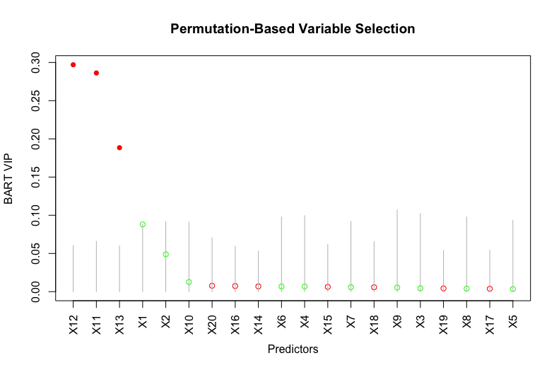
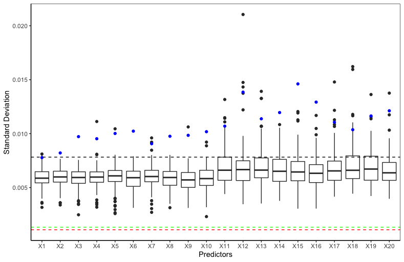
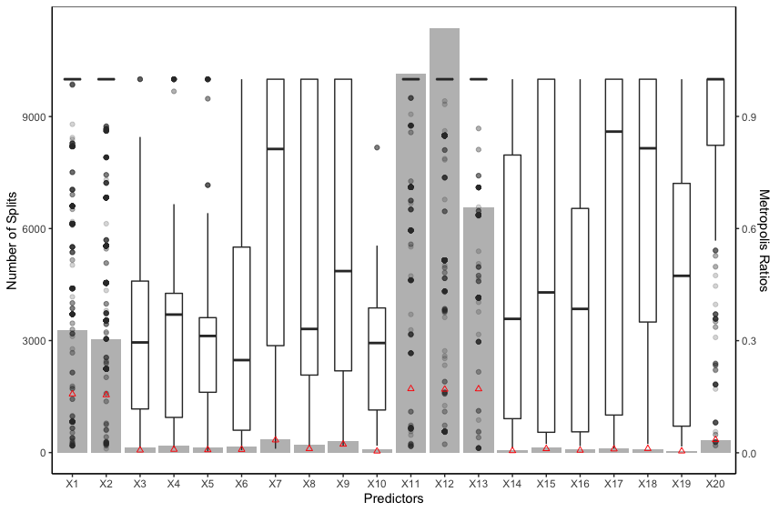
This example is a variant of Friedman’s example ([11]) where the predictors impact the response in a nonlinear and non-additive way. We modify Friedman’s example by changing the predictors and from continuous to binary. We fit a BART model on the observations with trees and obtain the VIPs based on posterior samples after burning in posterior samples. Since all the predictors are on the same scale , the binary predictor improves the fit of the response the same as the continuous predictor and the binary predictor moves the response more than the continuous predictor . However, Figure 1 shows that and have higher VIPs than and respectively, suggesting that BART VIP is biased against binary predictors. This issue occurs because a binary predictor has only one available splitting value while a continuous predictor has many more splitting values. As a result, continuous predictors appear more often in the ensemble.
2.2.2 Permutation-based variable selection with BART VIP
Apart from the bias issue of BART VIP, the original BART paper does not provide a complete variable selection approach in the sense that it does not provide a way of setting the threshold for BART VIPs to select predictors. In fact, [5] show that it is not possible to decide on an appropriate threshold for VIPs based on a single BART fit, because BART may fit noise due to its nonparametric flexibility. To deal with this, they develop a principled permutation-based variable selection approach which facilitates determining how large a BART VIP has to be in order to select a predictor.
Specifically, this approach first creates permutations of the response vector to form null datasets , where is a matrix of the observed predictors with each row corresponding to an observation, and then fits a BART model on each null dataset . As a result, vectors of BART VIPs , , can be obtained from the BART models. Since the null datasets delete the relationship between the response and predictors, the -dimensional vector can be regarded as a sample of the null distribution of the BART VIP for the predictor , which is the distribution of the BART VIP when the predictor is unrelated to the response . If the predictor is indeed not related to the response , then the true BART VIP obtained from the BART model on the original dataset follows the null distribution. Hence, predictors can be selected according to the relative location of their true BART VIPs in the corresponding null distributions. Since BART may fit noise, the true VIPs are estimated by the averaged VIPs which is the mean of multiple vectors of VIPs with each obtained from a replication of BART on the original dataset . [5] propose three criteria to select a subset of predictors. The least stringent one is the local threshold, i.e., the predictor is selected if the averaged VIP exceeds the quantile of the corresponding empirical distribution of the null distribution, where is a degenerate distribution at . The algorithm for a general permutation-based variable selection approach, not restricted to the one using BART VIP as the variable importance measure, is summarized in Algorithm 1.
This approach works well when all the predictors are continuous; however, it often fails to include relevant binary predictors when the predictors belong to different types and the number of predictors is small. Consider the following variant of Friedman’s example.
Example 2.
For each , sample from Bernoulli(0.5) independently, from Uniform(0,1) independently and from independently, where
Figure S.1 of the Supplementary Material shows that both the two relevant binary predictors and are not selected by this method. Further analysis is provided in Section 3.1.
2.2.3 Variable selection with DART
DART ([19]) is a variant of BART, which replaces the discrete uniform distribution for selecting a split variable with a categorical distribution of which the event probabilities follow a Dirichlet distribution. With the Dirichlet hyper-prior, probability mass is accumulated towards the predictors that are more frequently used along the MCMC iterations, thereby inducing sparsity and improving the predictive performance in high dimensional settings.
As discussed in Section 2.1, BART can be considered as a Bayesian model selection approach, so predictors can be selected by using the marginal posterior variable inclusion probability (MPVIP)
| (4) |
However, the model space explored by BART is not only all the possible combinations of the predictors, but also all the possible relationships that the sum-of-trees model can express using the predictors, which implies that the cardinality of the model space is much bigger than and that the variable selection results can be susceptible to the influence of noise predictors, especially when the number of predictors is large. DART avoids the influence of noise predictors by employing the shrinkage Dirichlet hyper-prior. DART estimates the MPVIP for a predictor by the proportion of the posterior samples of the trees structures where the predictor is used as a split variable at least once, and selects predictors with MPVIP at least , yielding a median probability model. [3] shows that the median probability model, rather than the most probable model, is the optimal choice in the sense that the predictions for future observations are closest to the Bayesian model averaging prediction in the squared error sense. However, the assumptions for this property are quite strong and often not realistic, including the assumption of an orthogonal predictors matrix.
2.2.4 Variable selection with ABC Bayesian forest
[23] introduce a spike-and-forest prior which wraps the BART prior with a spike-and-slab prior on the model space:
The tree-based model under the spike-and-forest prior can be used not only for estimation but also for variable selection, as shown in [20]. Due to the intractable marginal likelihood, they propose an approximate Bayesian computation (ABC) sampling method based on data-splitting to help sample from the model space with higher ABC acceptance rate. Specifically, at each iteration, the dataset is randomly split into a training set and a test set according to a certain split ratio. The algorithm proceeds by sampling a subset from the prior , fitting a BART model on the training set only with the predictors in , and computing the root mean squared errors (RMSE) for the test set based on a posterior sample from the fitted BART model. Only those subsets that result in a low RMSE on the test set are kept for selection. Similar to DART, ABC Bayesian forest selects predictors based on their MPVIP defined as (4) which is estimated by computing the proportion of ABC accepted BART posterior samples that use the predictor at least one time. Given the ’s, predictors with exceeding a pre-specified threshold are selected.
ABC Bayesian forest exhibits good performance in excluding irrelevant predictors, but it does not perform well in including relevant predictors in presence of correlated predictors, as shown in Section 4. One possible reason is that ABC Bayesian forest internally uses only one posterior sample after a short burn-in period and a small number of trees for BART, making it easy to miss relevant predictors. Furthermore, given that ABC Bayesian forest computes based on the ABC accepted BART posterior samples rather than the ABC accepted subsets, it appears that the good performance in excluding irrelevant predictors may be primarily due to the variable selection capability of BART itself, when the number of trees is small.
3 New Approaches
3.1 BART VIP with Type Information
In Section 2.2.2, we show an example where the approach of [5] fails to include relevant binary predictors. The intuition of this approach is that a relevant predictor is expected to appear more often in the model built on the original dataset than that built on a null dataset. In this section, we revisit Example 2 and show that the intuition does hold for both relevant continuous and relevant binary predictors, but that the increase in usage of a relevant binary predictor is often offset by the increase of relevant continuous predictors, when the number of predictors is not large, thereby making the true VIP of a relevant binary predictor insignificant with respect to (w.r.t.) the corresponding null VIPs. In light of this observation, we modify BART VIP with the type information of predictors to help identify relevant binary predictors.
Direct studying BART VIP is challenging because each consists of different components . To make the analysis more interpretable, we introduce an approximation of BART VIP, which only contains one component.
Definition 3.1 (Approximation of BART VIP).
Following the notation in Definition 2.1, for every and , let be the number of splitting nodes using the predictor over all the posterior samples of the trees structures and be the total number of splitting nodes over all the posterior samples. For each predictor , define
The following lemma shows that defined above can be used to approximate BART VIP under mild conditions.
Lemma 3.2.
For any and , let be the total number of splitting nodes in the posterior sample and be the average number of splitting nodes in a posterior sample. If and for some positive numbers , then the difference between and the corresponding BART VIP is bounded, i.e., .
Remark.
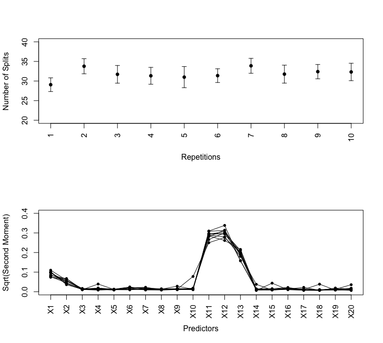
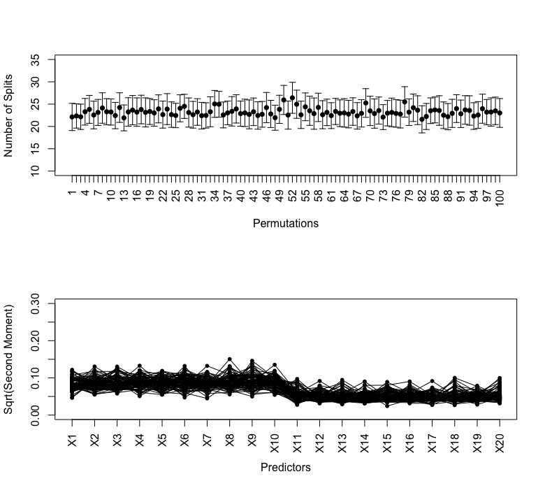
The first condition above means that the variance of , the proportion of the usage of the predictor in an ensemble, is bounded. The second condition means that the coefficient of variation of , the number of splitting nodes in an ensemble, is also bounded. Since [5] use posterior samples after a burn-in period, the variance of and the coefficient of variation of are small (see Figure S.2 of the Supplementary Material). Hence, Lemma 3.2 implies that can be used as an alternative to the corresponding BART VIP .
Proof.
See Section S.1 of the Supplementary Material. ∎
Consider the approach of [5]. For every , , and , let be the number of splitting nodes using the predictor in the posterior sample of the BART model built on the null dataset and be that of the repeated BART model built on the original dataset. Following the notation in Definition 3.1, write , , , and . By Lemma 3.2, for each predictor , we can use to approximate , the VIP obtained from the BART model on the null dataset, and to approximate , the VIP obtained from the repeated BART model on the original dataset. Denote by the averaged approximate VIP for the predictor across repetitions of BART on the original dataset. According to the local threshold of [5], a predictor is selected only if the average VIP exceeds the quantile of the empirical distribution , i.e.,
| (5) |
Similar to the approximation of BART VIP, we can approximate in (5) by and therefore the selection criteria (5) can be rewritten as
| (6) |
where and .
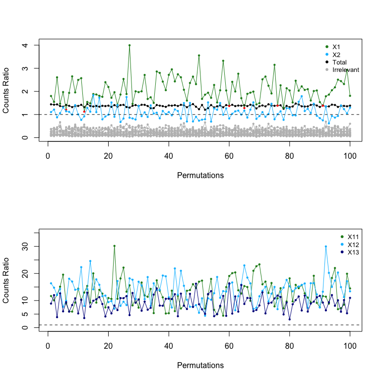
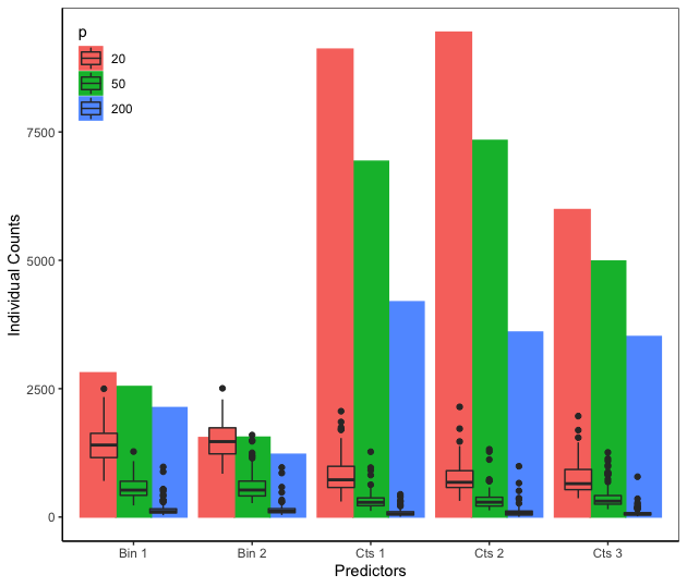
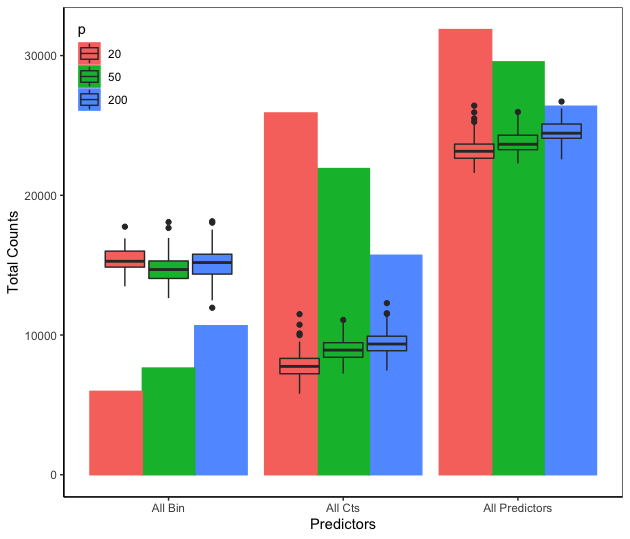
The ratio on the left hand side (LHS) of the inequality inside the sum of (6) represents the average increment in usage of a predictor in a BART model built on the original dataset, compared to a null dataset; the ratio on the right hand side (RHS) represents the average increment in the total number of the splitting nodes over all the posterior samples of a BART model built on the original dataset, compared to a null dataset. Figure S.3 of the Supplementary Material shows the overall counts ratio and the counts ratio for each predictor in Example 2. Both relevant continuous (, and ) and relevant binary ( and ) predictors are indeed used more frequently in the BART model built on the original dataset, i.e., , but the increment in usage of a relevant binary predictor is not always greater than the increment in the total number of splits, i.e., . A binary predictor can only be used once at most in each path of a tree because it only has one split value, and a few splits are sufficient to provide the information about a binary predictor. As a result, , the number of splits using a binary predictor, is limited by its low cardinality, even if it is relevant. In addition, the number of splits using a binary predictor in a BART model built on a null dataset is roughly of the total number of splits in the ensemble ([5]). As such, when the number of predictors is small, is close to (see the left subfigure of Figure S.4 of the Supplementary Material), thereby making the counts ratio for a binary predictor close to . The overall counts ratio is also close to because of the BART regularization prior. In fact, given a fixed number of trees in an ensemble, the total number of splits in the ensemble is controlled by the splitting probability, the probability of splitting a node into two child nodes, which is the same for BART models built on the original dataset and null datasets, so the total number of splits for the original dataset and a null dataset, and , are of similar magnitude (see the right subfigure of Figure S.4). As such, the increment in usage of a relevant binary predictor is easily offset by the increment in the total number of splits .
Figure S.4 of the Supplementary Material also shows that the increment in the total number of splits is primarily driven by those relevant continuous predictors, so essentially the increment in usage of a relevant binary predictor is offset by that of relevant continuous predictors. To alleviate this behavior, we modify Definition 2.1 using the type information of predictors.
Definition 3.3 (BART Within-Type Variable Inclusion Proportion).
Denote by (or ) the set of indicators for continuous (or binary) predictors. Following the notation in Definition 2.1, for every , let (or ) be the total number of splitting nodes using continuous (or binary) predictors in the posterior sample. For every , define the BART within-type VIP for the predictor as follows:
Define for any and . Write and . The permutation-based variable selection approach (Algorithm 1) using BART within-type VIP as the variable importance measure selects a predictor only if
| (7) |
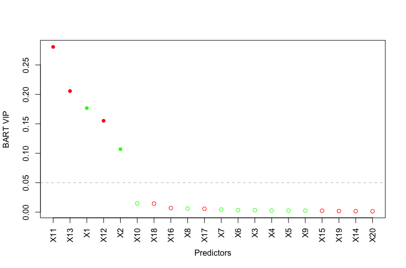
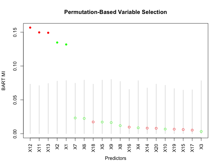
For a binary predictor, the selection criteria (7) removes the impact of continuous predictors, thereby not diluting the effect of a relevant binary predictor. Figure 2 shows the variable selection result of this approach. As opposed to the approach of [5], both the two relevant binary predictors and are clearly identified by this approach.
3.2 BART Variable Importance Using Metropolis Ratios
While BART within-type VIP works well in including relevant predictors in presence of a similar number of binary and continuous predictors, it becomes problematic if the number of predictors of one type is low. For example, when there are continuous predictors and binary predictor, the BART within-type VIP of the binary predictor is always for both the original dataset and a null dataset. As such, the binary predictor is never selected by the permutation-based approach, whether it is relevant or not. Furthermore, when there are more than two types of predictors, the computation of BART within-type VIP becomes complicated. Hence, we propose a new type of variable importance measure based on the Metropolis ratios calculated in the Metropolis-Hastings steps for sampling new trees, which are not affected by the issues above.
As mentioned in Section 2.1, a key feature of the Metropolis-within-Gibbs sampler is the Bayesian backfitting procedure for sampling , , where each is fit iteratively using the residual response , with all the other trees held constant. Thus, each can be obtained in two sequential steps:
where is the vector of residual responses. The distribution of has a closed form up to a normalizing constant and therefore can be sampled by a Metropolis-Hastings algorithm. [8] develop a Metropolis-Hastings algorithm that proposes a new tree based on the current tree using one of the four moves: BIRTH, DEATH, CHANGE and SWAP. The BIRTH and DEATH proposals are the essential moves for sufficient mixing of the Gibbs sampler, so both the CRAN R package BART ([24]) and our package BartMixVs ([22]) implement these two proposals, each with equal probability. A BIRTH proposal turns a terminal node into a splitting node and a DEATH proposal replaces a splitting node leading to two terminal nodes by a terminal node. Thus, the proposed tree is identical to the current tree except growing/pruning one splitting node.
We consider using the Metropolis ratio for accepting a BIRTH proposal to construct a variable importance measure. For convenience, we suppress the subscript in the following. The Metropolis ratio for accepting a BIRTH proposal at a terminal node of the current tree can be written as
| (8) |
where
| (9) |
The BART prior splits a node of depth into two child nodes of with probability for some and . Given that, the untruncated Metropolis ratio can be explicitly expressed as the product of three ratios:
| Nodes Ratio | ||||
| Depth Ratio | ||||
| Likelihood Ratio |
where is the number of terminal nodes in the current tree and is the depth of the node in the current tree . The derivation can be found in Section S.2 of the Supplementary Material.
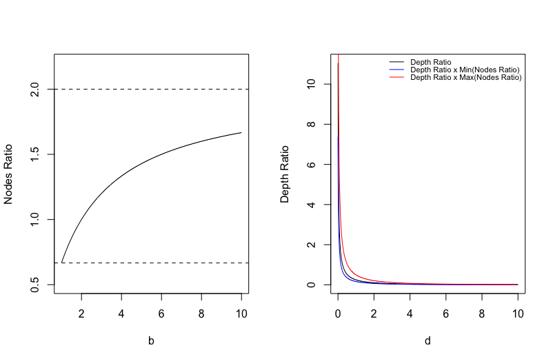
Figure S.5 of the Supplementary Material shows the nodes ratios for different numbers of terminal nodes and the depth ratios for different depths when the hyper-parameters and are set as default, i.e., and . From the figure, we can see that the product of nodes ratio and depth ratio is mostly affected by the depth ratio which decreases as the proposed depth increases, implying that assigns a greater value to a shallower node which typically contains more samples. Since the likelihood ratio indicates the conditional improvement to fitting brought by the new split, the untruncated Metropolis ratio considers both the proportion of samples affected at the node and the conditional improvement to fitting brought by the new split at the node . However, it is not appropriate to directly use to construct a variable importance measure, due to the occurrence of extremely large which dominates the others. Instead, we use the Metropolis ratio in (8) to construct the following BART Metropolis importance.
Definition 3.4 (BART Metropolis Importance).
Let be the number of posterior samples obtained from a BART model. For every and , define the average Metropolis acceptance ratio per splitting rule using the predictor at the posterior sample as follows:
where is the set of splitting nodes in the posterior sample of the tree and is the indicator of the split variable at the node . The BART Metropolis Importance (MI) for the predictor is defined as the normalized , averaged across posterior samples:
| (10) |
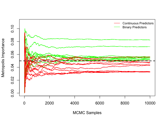
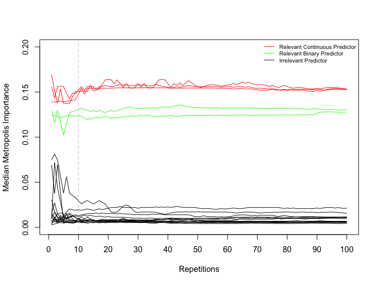
The intuition of BART MI is that a relevant predictor is expected to be consistently accepted with a high Metropolis ratio. Figure 3 shows that the Metropolis ratios of the splits using relevant predictors (, , , and ) as the split variable have a higher median and smaller standard error than those using irrelevant predictors, implying that relevant predictors are consistently accepted with a higher Metropolis ratio. BART MI and BART VIP have similar forms. The key difference is the “kernel” they use. While BART VIP uses the number of splits which tends to be biased against binary predictors, BART MI uses the average Metropolis acceptance ratio which is similar between the relevant binary predictors and relevant continuous predictors, as shown in Figure 3. Hence, the average Metropolis acceptance ratio not only helps BART MI distinguish relevant and irrelevant predictors, but also helps BART MI not be biased against predictors of a certain type.
The vector of average Metropolis acceptance ratios does not sum to and each of them varies from to . We normalize the vector in (10) based on the idea that ’s are correlated in the sense that once some predictors that explain the response more are accepted with higher Metropolis ratios, the rest of predictors will be accepted with lower Metropolis ratios or not be used. In addition, we take the average over posterior samples in (10) because averaging further helps identify relevant predictors. In fact, an irrelevant predictor can be accepted with a high Metropolis ratio at some MCMC iterations, but it can be quickly removed from the model by the DEATH proposal. As a result, the irrelevant predictor can have a few large ’s and many small ’s, thereby resulting in a small BART MI , as shown in Figure 3.
We further explore BART MI under null settings. We create a null dataset of Example 2 and fit a BART model on it. Figure S.6 of the Supplementary Material shows that not all the MIs, ’s, converge to , implying that may not be a good selection threshold for ’s. We repeat the experiment of [5] for BART MI under null settings to explore the variation among ’s. Specifically, we create null datasets of the data generated from Example 2, and for each null dataset, we run BART times with different initial values of the hyper-parameters. Let be the BART MI for the predictor from the BART model on the null dataset. We investigate three nested variances listed in Table 1.
| Variance | Description |
|---|---|
| The variability of BART MI for the predictor in the dataset; . | |
| The variability due to chance capitalization, i.e., fitting noise, of BART for the predictor across datasets; . | |
| The variability of BART MI across predictors; . |
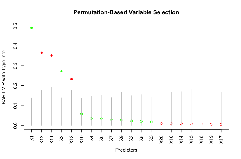
Results of the experiment are shown in Figure S.7 of the Supplementary Material. The non-zero ’s imply that there is variation in ’s among the repetitions of BART with different initial values, so it is necessary to average MIs over a certain number of repetitions of BART to get stable MIs. In practice, we find that among the repetitions of BART, irrelevant predictors occasionally get outliers of MI. Thus, instead of averaging MIs over BART repetitions, we take the median of them. Similar to [5], we also find that repetitions of BART is sufficient to get stable MIs (see Figure S.8 of the Supplementary Material). Figure S.7 also shows that the second type of standard deviation is significantly greater than the median of ’s for each predictor, which suggests that BART tends to overfit noise. Since the overall MI is always , the relatively large indicates that not all the are approximately , suggesting that it is not possible to determine a single selection threshold for all the MIs. Therefore, we employ the permutation-based approach (Algorithm 1) to select thresholds for each MI. A slight modification is applied to line 4 of Algorithm 1: we take the median, rather than the average, of BART MIs, over the repetitions of BART on the original dataset. The variable selection result of this approach for Example 2 is shown in Figure 4.
3.3 Backward Selection with Two Filters
In this section, we propose an approach to select a subset of predictors with which the BART model gives the best prediction. In general, to select the best subset of predictors from the model space consisting of possible models, one needs a search strategy over the model space and decision-making rules to compare models. Here we use the backward elimination approach to search the model space, mainly because it is a deterministic approach and is efficient with a moderate number of predictors. Typically, backward selection starts with the full model with all the predictors, followed by comparing the deletion of each predictor using a chosen model fit criterion and then deleting the predictor whose loss gives the most statistically insignificant deterioration of the model fit. This process is repeated until no further predictors can be deleted without a statistically insignificant loss of fit. Some popular model fit criterions such as AIC and BIC are not available for BART, because the maximum likelihood estimates are unavailable and the number of parameters in the model is hard to determine. To overcome this issue, we propose a backward selection approach with two easy-to-compute selection criterions as the decision-making rules.
We first split the dataset into a training set and a test set before starting the backward procedure. To measure the model fit, we make use of the mean squared errors (MSE) of the test set
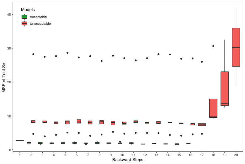
where is the estimated sum-of-trees function. Figure 5 shows that can distinguish between acceptable models and unacceptable models, where acceptable models are defined as those models including all the relevant predictors and unacceptable models are defined as those missing some relevant predictors. At each backward selection step, we run BART models on the training set and compute the MSE of the test set. The model with the smallest is chosen as the “winner” at that step. However, due to the lack of stopping rules under such nonparametric setting, the backward selection has to continue until there is only one predictor in the model, and ultimately returns “winner” models with different model sizes ranging from to .
Given the “winner” models, we compare them using the expected log pointwise predictive density based on leave-one-out (LOO) cross validation:
| (11) |
where , represents the set of BART parameters, is the predictive density of given , is the likelihood of , and is the posterior density of BART given the observations . The quantity not only measures the predictive capability of a model, but also penalizes the complexity of the model, i.e., the number of predictors used in the model. Hence, we choose the model with the largest as the best model.
Direct computing (11) involves fitting BART times. To avoid this, we use the approach of [27] that estimates each using importance sampling with the full posterior distribution as the sampling distribution and the smoothed ratios as the importance ratios, where are the posterior samples from the full posterior distribution . The smoothness is achieved by fitting a generalized Pareto distribution to the upper tail of each set of the importance ratios , . Thus, in (11) can be estimated by using the likelihoods based on posterior samples from the BART model fit on the dataset , where is the posterior sample of the sum-of-trees function (2) and is the normal density with mean and standard error .
The approach above can also be extended to the probit BART model (3) by changing the to the mean log loss (MLL) of the test set
| (12) |
and replacing the normal likelihoods with the Bernoulli density , where is the estimated probability based on the posterior sample of probit BART for the observation and . We summarize this algorithm in Algorithm 2. Although this algorithm requires fitting BART times, models at the same backward selection step can be fitted in parallel, which implies that the time complexity can be reduced to if there are sufficient computing resources.
4 Simulations
In this section, we compare the proposed variable selection approaches: (1) permutation-based approach using within-type BART VIP, (2) permutation-based approach using BART MI, and (3) backward selection with two filters, with the existing BART-based variable selection approaches: (4) median probability model from DART, (5) permutation-based approach using BART VIP, and (6) ABC Bayesian forest. For the permutation-based approaches (1), (2) and (5), we set , and (see Algorithm 1), and use trees for BART to encourage competition among the predictors. The three permutation-based approaches are based on the same posterior samples and the one using within-type BART VIP is only applied to scenarios with mixed-type predictors. For the backward selection procedure (3), we set (see Algorithm 2) and use trees for BART to ensure its prediction power. For DART (4), we consider and trees, respectively. For ABC Bayesian forest, as [20] suggest, we assume the prior on the model space to be the beta-binomial prior with , set the split ratio as , and use and trees for BART respectively; we generate ABC samples, rank the samples by MSE in ascending order if the response variable is continuous (or by MLL if the response variable is binary), and keep the top of samples for selection; we report selection results for two selection thresholds and . All the methods above, except ABC Bayesian forest, burn in the first 1000 and keep 1000 posterior samples in each BART run. ABC Bayesian forest burns in posterior samples and saves the posterior sample, as [20] suggest. Other hyper-parameters of BART are the same as the default recommended by [9]. The simulation results were obtained using the R package BartMixVs ([22]) which is briefly introduced in Section S.3 of the Supplementary Material.
To evaluate variable selection results, we consider precision (prec), recall (rec), score, and the proportion of the replications that miss at least one relevant predictor (), given by
where TP is the number of relevant predictors correctly selected, FP is the number of predictors incorrectly selected and FN is the number of relevant predictors not selected. High precision indicates good ability of excluding irrelevant predictors and high recall indicates good ability of including relevant predictors. The score is a balanced score between precision and recall. The lowest score is , implying that the method does not miss any relevant predictors over all the replications.
We evaluate the aforementioned variable selection approaches under four possible combination scenarios of . Each scenario is replicated 100 times. The simulation results for the scenario of binary response and continuous predictors can be found in Section S.4.2 of the Supplementary Material.
4.1 Continuous Response and Continuous Predictors
In this setting, we consider two scenarios. Scenario C.C.1 is an example from [11]; Scenario C.C.2, which includes correlation between predictors, is borrowed from [29]. For both of them, we consider , and .
Scenario C.C.1.
Sample the predictors from independently and the response from , where
| (13) |
Scenario C.C.2.
Sample the predictors from with , , and the response from , where
| (14) |
Results are given in Table 2. When the predictors are independent (Scenario C.C.1) and , none of the methods miss any relevant predictors, i.e., and . The permutation-based approach using BART VIP and the ABC Bayesian forest methods, except the one using trees and selection threshold (i.e., ABC-20-0.25), are the best in terms of precision and the scores, followed by the permutation-based approach using BART MI and DART with trees. When , only the ABC Bayesian forest with trees and selection threshold (i.e., ABC-10-0.50) fails to include all the relevant predictors. As discussed in Section 2.2.4, ABC Bayesian forest using a small number of trees and keeping a small number of posterior samples makes it easy to miss relevant predictors, especially when the number of predictors is large and the selection threshold is high. As shown in Table 2, increasing the number of trees to or decreasing the selection threshold to can improve the result. The other three ABC Bayesian forest methods achieve the best precision and scores, followed by the two permutation-based approaches. The backward selection procedure is not a top choice in terms of precision, but its precision ( for and for ) is acceptable in the sense that it only includes about irrelevant predictors on average. In fact, we find that the LOO score used in the backward selection, though penalizing the model complexity, appears to have difficulty in distinguishing between the true model and an acceptable model with a similar number of predictors, thereby resulting in a relatively low precision score.
| Scenario C.C.1 | |||||||||
| rec | prec | rec | prec | ||||||
| DART-20 | 0 | 1(0) | 0.87(0.01) | 0.93(0.01) | 0 | 1(0) | 0.86(0.01) | 0.92(0.01) | |
| DART-200 | 0 | 1(0) | 0.7(0.02) | 0.81(0.01) | 0 | 1(0) | 0.63(0.02) | 0.76(0.01) | |
| ABC-10-0.25 | 0 | 1(0) | 1(0) | 1(0) | 0 | 1(0) | 1(0) | 1(0) | |
| ABC-10-0.50 | 0 | 1(0) | 1(0) | 1(0) | 0.33 | 0.93(0.01) | 1(0) | 0.96(0.01) | |
| ABC-20-0.25 | 0 | 1(0) | 0.5(0.01) | 0.66(0.01) | 0 | 1(0) | 1(0) | 1(0) | |
| ABC-20-0.50 | 0 | 1(0) | 1(0) | 1(0) | 0 | 1(0) | 1(0) | 1(0) | |
| Permute (VIP) | 0 | 1(0) | 1(0) | 1(0) | 0 | 1(0) | 0.95(0.01) | 0.97(0) | |
| Permute (MI) | 0 | 1(0) | 0.98(0.01) | 0.99(0) | 0 | 1(0) | 0.94(0.01) | 0.97(0.01) | |
| Backward | 0 | 1(0) | 0.75(0.02) | 0.83(0.02) | 0 | 1(0) | 0.74(0.02) | 0.83(0.02) | |
| Scenario C.C.2 | |||||||||
| rec | prec | rec | prec | ||||||
| DART-20 | 0.43 | 0.8(0.03) | 0.86(0.02) | 0.8(0.02) | 0.97 | 0.37(0.03) | 0.47(0.04) | 0.39(0.03) | |
| DART-200 | 0 | 1(0) | 0.83(0.02) | 0.9(0.01) | 0.64 | 0.65(0.03) | 0.49(0.03) | 0.53(0.03) | |
| ABC-10-0.25 | 0.02 | 1(0) | 0.69(0.02) | 0.8(0.01) | 1 | 0.08(0.01) | 0.28(0.04) | 0.13(0.02) | |
| ABC-10-0.50 | 0.82 | 0.61(0.02) | 0.98(0.01) | 0.73(0.02) | 1 | 0(0) | 0.02(0.01) | 0.01(0.01) | |
| ABC-20-0.25 | 0 | 1(0) | 0.12(0) | 0.22(0) | 0.99 | 0.28(0.02) | 0.45(0.04) | 0.33(0.03) | |
| ABC-20-0.50 | 0.1 | 0.97(0.01) | 0.97(0.01) | 0.97(0.01) | 1 | 0.01(0) | 0.04(0.02) | 0.02(0.01) | |
| Permute (VIP) | 0 | 1(0) | 0.98(0.01) | 0.99(0) | 0.71 | 0.68(0.03) | 0.26(0.01) | 0.37(0.01) | |
| Permute (MI) | 0 | 1(0) | 0.89(0.01) | 0.93(0.01) | 0.93 | 0.43(0.03) | 0.27(0.02) | 0.32(0.02) | |
| Backward | 0 | 1(0) | 0.86(0.02) | 0.92(0.01) | 0.02 | 0.99(0.01) | 0.79(0.03) | 0.84(0.03) | |
When the predictors are correlated (Scenario C.C.2) and , the two permutation-based approaches, the backward selection approach, DART with trees, and the ABC-20-0.25 approach successfully identify all the relevant predictors for all the replications; the first four of them have competitive precision and scores. When more correlated and irrelevant predictors are included , the backward selection procedure has superior performance in all metrics. It identifies all the relevant predictors for of the times and achieves the highest precision () and scores (). Compared with the independent setting (Scenario C.C.1), ABC Bayesian forest suffers the most from the multicollinearity as we found that this approach often does not select out any predictors.
With the first three examples in Table 2 being considered, the two proposed approaches along with the approach of [5] and DART with trees consistently perform well in identifying all the relevant predictors. For Scenario C.C.2 with predictors, the backward selection approach significantly outperforms other methods.
4.2 Continuous Response and Mixed-Type Predictors
In this setting, we consider Scenario C.M.1, a modified Friedman’s example, and Scenario C.M.2, an example including correlation between predictors. We consider , and for Scenario C.M.1, and and for Scenario C.M.2.
Scenario C.M.1.
Sample the predictors from independently, from independently, and the response from , where
| (15) |
Scenario C.M.2.
Sample the predictors from independently, from Bernoulli(0.5) independently, from a multivariate normal distribution with mean , variance and correlation , and the response from , where
| (16) |
We report the simulation results for Scenario C.M.1 with the settings, , and , and Scenario C.M.2 with the settings, and , in Table 3. Simulation results for other settings are reported in Table S.1 of the Supplementary Material.
| Scenario C.M.1 | |||||||||
| rec | prec | rec | prec | ||||||
| DART-20 | 0 | 1(0) | 0.96(0.01) | 0.98(0) | 0 | 1(0) | 0.95(0.01) | 0.97(0) | |
| DART-200 | 0 | 1(0) | 0.65(0.02) | 0.78(0.01) | 0 | 1(0) | 0.63(0.02) | 0.76(0.01) | |
| ABC-10-0.25 | 0 | 1(0) | 0.99(0) | 0.99(0) | 0 | 1(0) | 1(0) | 1(0) | |
| ABC-10-0.50 | 0 | 1(0) | 1(0) | 1(0) | 0.56 | 0.89(0.01) | 1(0) | 0.94(0.01) | |
| ABC-20-0.25 | 0 | 1(0) | 0.62(0.01) | 0.76(0.01) | 0 | 1(0) | 0.95(0.01) | 0.97(0) | |
| ABC-20-0.50 | 0 | 1(0) | 1(0) | 1(0) | 0 | 1(0) | 1(0) | 1(0) | |
| Permute (VIP) | 0.29 | 0.94(0.01) | 1(0) | 0.97(0.01) | 0 | 1(0) | 0.85(0.01) | 0.91(0.01) | |
| Permute (Within-Type VIP) | 0 | 1(0) | 0.99(0.01) | 0.99(0) | 0 | 1(0) | 0.73(0.02) | 0.84(0.01) | |
| Permute (MI) | 0 | 1(0) | 0.97(0.01) | 0.98(0) | 0 | 1(0) | 0.82(0.01) | 0.9(0.01) | |
| Backward | 0 | 1(0) | 0.76(0.02) | 0.84(0.02) | 0 | 1(0) | 0.82(0.02) | 0.88(0.02) | |
| Scenario C.M.2 | |||||||||
| rec | prec | rec | prec | ||||||
| DART-20 | 0.37 | 0.94(0.01) | 0.91(0.01) | 0.92(0.01) | 0.09 | 0.98(0) | 0.91(0.01) | 0.94(0.01) | |
| DART-200 | 0.17 | 0.97(0.01) | 0.49(0.01) | 0.64(0.01) | 0.01 | 1(0) | 0.58(0.01) | 0.73(0.01) | |
| ABC-10-0.25 | 0.95 | 0.81(0.01) | 0.94(0.01) | 0.87(0.01) | 0.54 | 0.91(0.01) | 0.99(0) | 0.94(0) | |
| ABC-10-0.50 | 1 | 0.69(0.01) | 1(0) | 0.81(0.01) | 0.96 | 0.82(0.01) | 1(0) | 0.9(0) | |
| ABC-20-0.25 | 0.57 | 0.9(0.01) | 0.44(0.01) | 0.58(0.01) | 0.05 | 0.99(0) | 0.69(0.01) | 0.8(0.01) | |
| ABC-20-0.50 | 1 | 0.78(0.01) | 0.99(0) | 0.87(0.01) | 0.7 | 0.88(0.01) | 1(0) | 0.93(0) | |
| Permute (VIP) | 0.18 | 0.97(0.01) | 0.93(0.01) | 0.95(0.01) | 0.51 | 0.9(0.01) | 0.96(0.01) | 0.93(0.01) | |
| Permute (Within-Type VIP) | 0.44 | 0.93(0.01) | 0.86(0.02) | 0.89(0.01) | 0.06 | 0.99(0.01) | 0.92(0.01) | 0.95(0.01) | |
| Permute (MI) | 0.07 | 0.99(0) | 0.85(0.01) | 0.91(0.01) | 0 | 1(0) | 0.89(0.01) | 0.94(0.01) | |
| Backward | 0.11 | 0.98(0.01) | 0.47(0.03) | 0.57(0.03) | 0 | 1(0) | 0.75(0.02) | 0.83(0.02) | |
When the predictors are independent (Scenario C.M.1) and , all the methods, except the permutation-based approach using BART VIP, are able to identify all the relevant predictors. The two proposed permutation-based approaches, DART with trees, and the ABC Bayesian forest approaches except ABC-20-0.25 have comparable best precision and scores, followed by the backward selection procedure. When the dimension is increased to , the ABC-10-0.50 method again fails to include all the relevant predictors, like Scenario C.C.1. The permutation-based approach using BART VIP does not perform poorly in this case, because as gets larger, stays in a similar magnitude and gets smaller (see the left subfigure of Figure S.4 of the Supplementary Material). As such, the offset effect discussed in Section 3.1 disappears. The three proposed approaches are still able to identify all the relevant predictors, but their precision scores are slightly worse than other methods.
When the mixed-type predictors are correlated (Scenario C.M.2), variable selection becomes more challenging. When , the permutation-based approach using BART MI and the backward selection procedure are the best in terms of the and recall scores. Furthermore, only these two methods successfully identify all the relevant predictors over all the replications when . When high noise is included, all the methods have difficulty identifying all the true predictors.
In terms of of the recall and scores, the permutation-based approach using BART MI and the backward selection approach are always the top choices for all the examples in Table 3 and Table S.1, except Scenario C.M.2 with . Compared to the other two proposed approaches, the permutation-based approach using BART within-type VIP suffers from multicollinearity, though it does improve the approach of [5] in presence of a small number of mixed-type predictors.
4.3 Binary Response and Mixed-Type Predictors
In this setting, we consider two scenarios, Scenario B.M.1 and Scenario B.M.2. For Scenario B.M.1, we consider and ; for Scenario B.M.2, we consider .
Scenario B.M.1.
Sample the predictors from independently, from independently, and the response from , where is defined in (15).
Scenario B.M.2.
Sample the predictors from independently, from Bernoulli(0.5) independently, from a multivariate normal distribution with mean , variance and correlation , and the response from , where is defined in (16).
| Scenario B.M.1 | |||||||||
| rec | prec | rec | prec | ||||||
| DART-20 | 0.26 | 0.95(0.01) | 0.99(0.01) | 0.96(0.01) | 0.65 | 0.87(0.01) | 0.99(0) | 0.92(0.01) | |
| DART-200 | 0.13 | 0.97(0.01) | 0.75(0.02) | 0.83(0.01) | 0.53 | 0.89(0.01) | 0.79(0.02) | 0.83(0.01) | |
| ABC-10-0.25 | 0.55 | 0.89(0.01) | 0.87(0.01) | 0.87(0.01) | 1 | 0.8(0) | 0.98(0.01) | 0.88(0) | |
| ABC-10-0.50 | 0.97 | 0.81(0) | 1(0) | 0.89(0) | 1 | 0.69(0.01) | 1(0) | 0.81(0.01) | |
| ABC-20-0.25 | 0.03 | 0.99(0) | 0.18(0) | 0.31(0) | 0.92 | 0.82(0.01) | 0.85(0.01) | 0.83(0.01) | |
| ABC-20-0.50 | 0.85 | 0.83(0.01) | 0.98(0.01) | 0.9(0) | 1 | 0.78(0.01) | 0.99(0) | 0.87(0) | |
| Permute (VIP) | 0.1 | 0.98(0.01) | 0.99(0) | 0.99(0) | 0.16 | 0.97(0.01) | 0.81(0.01) | 0.88(0.01) | |
| Permute (Within-Type VIP) | 0.08 | 0.98(0.01) | 1(0) | 0.99(0) | 0.22 | 0.96(0.01) | 0.8(0.02) | 0.87(0.01) | |
| Permute (MI) | 0.1 | 0.98(0.01) | 0.96(0.01) | 0.97(0.01) | 0.25 | 0.95(0.01) | 0.79(0.01) | 0.86(0.01) | |
| Backward | 0.09 | 0.98(0.01) | 0.93(0.02) | 0.94(0.01) | 0.37 | 0.93(0.01) | 0.87(0.02) | 0.88(0.01) | |
| rec | prec | rec | prec | ||||||
| DART-20 | 0.01 | 1(0) | 0.98(0.01) | 0.99(0) | 0.17 | 0.97(0.01) | 0.98(0.01) | 0.97(0.01) | |
| DART-200 | 0 | 1(0) | 0.95(0.01) | 0.97(0.01) | 0.03 | 0.99(0) | 0.95(0.01) | 0.97(0.01) | |
| ABC-10-0.25 | 0.01 | 1(0) | 0.95(0.01) | 0.97(0.01) | 0.82 | 0.84(0.01) | 0.99(0) | 0.9(0) | |
| ABC-10-0.50 | 0.53 | 0.89(0.01) | 1(0) | 0.94(0.01) | 1 | 0.8(0) | 1(0) | 0.89(0) | |
| ABC-20-0.25 | 0 | 1(0) | 0.24(0) | 0.39(0) | 0.22 | 0.96(0.01) | 0.91(0.01) | 0.93(0.01) | |
| ABC-20-0.50 | 0.02 | 1(0) | 0.99(0) | 0.99(0) | 0.96 | 0.81(0) | 1(0) | 0.89(0) | |
| Permute (VIP) | 0 | 1(0) | 1(0) | 1(0) | 0 | 1(0) | 0.85(0.01) | 0.92(0.01) | |
| Permute (Within-Type VIP) | 0 | 1(0) | 0.99(0) | 1(0) | 0 | 1(0) | 0.85(0.02) | 0.91(0.01) | |
| Permute (MI) | 0 | 1(0) | 0.96(0.01) | 0.98(0) | 0 | 1(0) | 0.82(0.01) | 0.89(0.01) | |
| Backward | 0 | 1(0) | 0.91(0.01) | 0.95(0.01) | 0 | 1(0) | 0.9(0.01) | 0.94(0.01) | |
| Scenario B.M.2 | |||||||||
| rec | prec | rec | prec | ||||||
| DART-20 | 0.95 | 0.75(0.01) | 0.91(0.01) | 0.82(0.01) | 0.62 | 0.89(0.01) | 0.93(0.01) | 0.91(0.01) | |
| DART-200 | 0.98 | 0.75(0.01) | 0.32(0.01) | 0.44(0.01) | 0.56 | 0.9(0.01) | 0.52(0.02) | 0.65(0.01) | |
| ABC-10-0.25 | 1 | 0.71(0.01) | 0.85(0.01) | 0.76(0.01) | 1 | 0.81(0.01) | 0.93(0.01) | 0.86(0.01) | |
| ABC-10-0.50 | 1 | 0.53(0.01) | 1(0) | 0.69(0.01) | 1 | 0.71(0.01) | 1(0) | 0.83(0.01) | |
| ABC-20-0.25 | 0.98 | 0.8(0.01) | 0.22(0) | 0.34(0) | 0.78 | 0.87(0.01) | 0.33(0.01) | 0.48(0.01) | |
| ABC-20-0.50 | 1 | 0.62(0.01) | 0.96(0.01) | 0.75(0.01) | 1 | 0.77(0.01) | 0.98(0.01) | 0.86(0.01) | |
| Permute (VIP) | 0.93 | 0.8(0.01) | 0.81(0.01) | 0.8(0.01) | 0.28 | 0.95(0.01) | 0.91(0.01) | 0.93(0.01) | |
| Permute (Within-Type VIP) | 0.96 | 0.79(0.01) | 0.83(0.02) | 0.8(0.01) | 0.52 | 0.91(0.01) | 0.87(0.02) | 0.88(0.01) | |
| Permute (MI) | 0.94 | 0.8(0.01) | 0.79(0.01) | 0.79(0.01) | 0.36 | 0.94(0.01) | 0.84(0.01) | 0.88(0.01) | |
| Backward | 0.67 | 0.84(0.01) | 0.54(0.03) | 0.57(0.03) | 0.15 | 0.97(0.01) | 0.55(0.03) | 0.63(0.03) | |
Simulation results are shown in Table 4. In presence of binary responses and mixed-type predictors, the variable selection results are clearly improved by increasing the sample size from to . Under the independent setting (Scenario B.M.1), the three proposed approaches along with the approach of [5] achieve and for both and , with samples. DART with trees gets slightly worse and recall scores under these two settings. However, when correlation is introduced, none of the methods work very well in identifying all the relevant predictors, though the backward selection procedure still gets the best recall and scores. In fact, we find that the result of the backward selection procedure can be greatly improved by thinning the MCMC chain of BART. For the Scenario B.M.2 with , we get , , and by keeping every posterior sample in each BART run.
4.4 Conclusion of Simulation Results
We summarize the simulation results above and in Section S.4 of the Supplementary Material in Table 5. We call a variable selection approach with no greater than and precision no less than , i.e., an approach with excellent capability of including all the relevant predictors and acceptable capability of excluding irrelevant predictors, a successful approach, and check it in Table 5. From the table, we can see that the backward selection approach achieves the highest success rate, followed by the two new permutation-based approaches, meaning that the three proposed approaches consistently perform well in identifying all the relevant predictors and excluding irrelevant predictors. A drawback of the three proposed approaches is that, like existing BART-based variable selection approaches, they also suffer from multicollinearity (Scenario C.M.2, Scenario B.C.2 and Scenario B.M.2), especially when the noise is high or the response is binary. Another shortcoming of the backward selection approach is the computational cost of running BART multiple times, but it should be noted that at each step of the backward selection, BART models can be fitted in parallel on multiple cores.
| Evaluated Setting | Evaluated Variable Selection Approaches | |||||||||||
|---|---|---|---|---|---|---|---|---|---|---|---|---|
| Scenario | DART-20 | DART-200 | ABC-10-0.25 | ABC-10-0.50 | ABC-20-0.25 | ABC-20-0.50 | Permute (VIP) | Permute (Within-Type VIP) | Permute (MI) | Backward | ||
| C.C.1 | ||||||||||||
| C.C.1 | ||||||||||||
| C.C.2 | ||||||||||||
| C.C.2 | ||||||||||||
| C.M.1 | ||||||||||||
| C.M.1 | ||||||||||||
| C.M.1 | ||||||||||||
| C.M.1 | ||||||||||||
| C.M.1 | ||||||||||||
| C.M.1 | ||||||||||||
| C.M.2 | ||||||||||||
| C.M.2 | ||||||||||||
| C.M.2 | ||||||||||||
| C.M.2 | ||||||||||||
| B.C.1 | ||||||||||||
| B.C.1 | ||||||||||||
| B.C.2 | ||||||||||||
| B.C.2 | ||||||||||||
| B.M.1 | ||||||||||||
| B.M.1 | ||||||||||||
| B.M.1 | ||||||||||||
| B.M.1 | ||||||||||||
| B.M.2 | ||||||||||||
| B.M.2 | ||||||||||||
| Success rate | ||||||||||||
5 Discussion and Future Work
This paper reviews and explores existing BART-based variable selection methods and introduces three new variable selection approaches. These new approaches are designed for adapting to data with mixed-type predictors, and more importantly, for better allowing all the relevant predictors into the model.
We outline some interesting areas for future work. First, the distribution of the null importance scores in the permutation-based approach is unknown. If the distribution can be approximated appropriately, then a better threshold can be used. Second, from the simulation studies for the backward selection approach, we note that there is only a slight difference in between the winner models from two consecutive steps, when both of them include all the relevant predictors. However, if one of the winner models drops a relevant predictor, the difference can become very large. In light of this, it would be advantageous to develop a formal stopping rule, which would also improve the precision score and the efficiency of the backward selection approach. Finally, a potential direction of conducting variable selection based on BART is to take further advantage of the model selection property of BART itself. As discussed in Section 2.1, BART can be regarded as a Bayesian model selection approach, but it does not perform well due to a large number of noise predictors. We may alleviate this issue by muting noise predictors adaptively and externally ([29]).
Acknowledgements
Luo and Daniels were partially supported by NIH R01CA 183854.
References
- [1] James H. Albert and Siddhartha Chib “Bayesian analysis of binary and polychotomous response data” In J. Amer. Statist. Assoc. 88.422, 1993, pp. 669–679 URL: http://links.jstor.org/sici?sici=0162-1459(199306)88:422%3C669:BAOBAP%3E2.0.CO;2-T&origin=MSN
- [2] André Altmann, Laura Toloşi, Oliver Sander and Thomas Lengauer “Permutation importance: a corrected feature importance measure” In Bioinformatics 26.10, 2010, pp. 1340–1347 DOI: 10.1093/bioinformatics/btq134
- [3] Maria Maddalena Barbieri and James O. Berger “Optimal predictive model selection” In Ann. Statist. 32.3, 2004, pp. 870–897 DOI: 10.1214/009053604000000238
- [4] Anirban Bhattacharya, Debdeep Pati, Natesh S. Pillai and David B. Dunson “Dirichlet-Laplace priors for optimal shrinkage” In J. Amer. Statist. Assoc. 110.512, 2015, pp. 1479–1490 DOI: 10.1080/01621459.2014.960967
- [5] Justin Bleich, Adam Kapelner, Edward I. George and Shane T. Jensen “Variable selection for BART: an application to gene regulation” In Ann. Appl. Stat. 8.3, 2014, pp. 1750–1781 DOI: 10.1214/14-AOAS755
- [6] Leo Breiman “Random forests” In Machine learning 45.1 Springer, 2001, pp. 5–32
- [7] Carlos M. Carvalho, Nicholas G. Polson and James G. Scott “The horseshoe estimator for sparse signals” In Biometrika 97.2, 2010, pp. 465–480 DOI: 10.1093/biomet/asq017
- [8] Hugh A. Chipman, Edward I. George and Robert E. McCulloch “Bayesian CART Model Search” In J. Amer. Statist. Assoc. 93.443 Taylor & Francis, 1998, pp. 935–948 DOI: 10.1080/01621459.1998.10473750
- [9] Hugh A. Chipman, Edward I. George and Robert E. McCulloch “BART: Bayesian additive regression trees” In Ann. Appl. Stat. 4.1, 2010, pp. 266–298 DOI: 10.1214/09-AOAS285
- [10] M.. Efroymson “Multiple regression analysis” In Mathematical methods for digital computers Wiley, New York, 1960, pp. 191–203
- [11] Jerome H. Friedman “Multivariate adaptive regression splines” With discussion and a rejoinder by the author In Ann. Statist. 19.1, 1991, pp. 1–141 DOI: 10.1214/aos/1176347963
- [12] Jerome H. Friedman “Greedy function approximation: a gradient boosting machine” In Ann. Statist. 29.5, 2001, pp. 1189–1232 DOI: 10.1214/aos/1013203451
- [13] Jerome H. Friedman “Stochastic gradient boosting” In Comput. Statist. Data Anal. 38.4, 2002, pp. 367–378 DOI: 10.1016/S0167-9473(01)00065-2
- [14] Stuart Geman and Donald Geman “Stochastic Relaxation, Gibbs Distributions, and the Bayesian Restoration of Images” In IEEE PAMI PAMI-6.6, 1984, pp. 721–741 DOI: 10.1109/TPAMI.1984.4767596
- [15] Edward I George and Robert E McCulloch “Variable Selection via Gibbs Sampling” In J. Amer. Statist. Assoc. 88.423 Taylor & Francis, 1993, pp. 881–889 DOI: 10.1080/01621459.1993.10476353
- [16] Trevor Hastie and Robert Tibshirani “Bayesian backfitting (with comments and a rejoinder by the authors” In Statist. Sci. 15.3 Institute of Mathematical Statistics, 2000, pp. 196–223 DOI: 10.1214/ss/1009212815
- [17] W.. Hastings “Monte Carlo sampling methods using Markov chains and their applications” In Biometrika 57.1, 1970, pp. 97–109 DOI: 10.1093/biomet/57.1.97
- [18] Adam Kapelner and Justin Bleich “bartMachine: Machine Learning with Bayesian Additive Regression Trees” In J. Stat. Softw. 70.4, 2016, pp. 1–40 DOI: 10.18637/jss.v070.i04
- [19] Antonio R. Linero “Bayesian regression trees for high-dimensional prediction and variable selection” In J. Amer. Statist. Assoc. 113.522, 2018, pp. 626–636 DOI: 10.1080/01621459.2016.1264957
- [20] Yi Liu, Veronika Ročková and Yuexi Wang “Variable selection with ABC Bayesian forests” In J. R. Stat. Soc. Ser. B. Stat. Methodol. 83.3, 2021, pp. 453–481 DOI: 10.1111/rssb.12423
- [21] Gilles Louppe “Understanding random forests” In Cornell University Library, 2014
- [22] Chuji Luo and Michael J. Daniels “The BartMixVs R package”, 2021 URL: https://github.com/chujiluo/BartMixVs
- [23] Veronika Ročková and Stéphanie Pas “Posterior concentration for Bayesian regression trees and forests” In Ann. Statist. 48.4, 2020, pp. 2108–2131 DOI: 10.1214/19-AOS1879
- [24] Rodney Sparapani, Charles Spanbauer and Robert McCulloch “Nonparametric machine learning and efficient computation with bayesian additive regression trees: the BART R package” In J. Stat. Softw. 97.1, 2021, pp. 1–66
- [25] Carolin Strobl, Anne-Laure Boulesteix, Achim Zeileis and Torsten Hothorn “Bias in random forest variable importance measures: Illustrations, sources and a solution” In BMC bioinformatics 8.1 Springer, 2007, pp. 25 DOI: 10.1186/1471-2105-8-25
- [26] Robert Tibshirani “Regression shrinkage and selection via the lasso” In J. Roy. Statist. Soc. Ser. B 58.1, 1996, pp. 267–288 URL: http://links.jstor.org/sici?sici=0035-9246(1996)58:1%3C267:RSASVT%3E2.0.CO;2-G&origin=MSN
- [27] Aki Vehtari, Andrew Gelman and Jonah Gabry “Erratum to: Practical Bayesian model evaluation using leave-one-out cross-validation and WAIC [ MR3647105]” In Stat. Comput. 27.5, 2017, pp. 1433 DOI: 10.1007/s11222-016-9709-3
- [28] Chi Wang, Giovanni Parmigiani and Francesca Dominici “Bayesian effect estimation accounting for adjustment uncertainty” In Biometrics 68.3, 2012, pp. 680–686 DOI: 10.1111/j.1541-0420.2011.01735.x
- [29] Ruoqing Zhu, Donglin Zeng and Michael R. Kosorok “Reinforcement learning trees” In J. Amer. Statist. Assoc. 110.512, 2015, pp. 1770–1784 DOI: 10.1080/01621459.2015.1036994
- [30] Hui Zou and Trevor Hastie “Regularization and variable selection via the elastic net” In J. R. Stat. Soc. Ser. B Stat. Methodol. 67.5, 2005, pp. 768 DOI: 10.1111/j.1467-9868.2005.00527.x
Supplement to "Variable Selection Using Bayesian Additive Regression Trees"
S.1 Proof of Lemma 3.2
Proof.
From Cauchy-Schwarz inequality, Definition 2.1 and Definition 3.1 of the main paper, it is clear that
∎
S.2 Decomposition of Untruncated Metropolis Ratio
The untruncated Metropolis ratio in Equation (9) of the main paper can be explicitly expressed as
where is the number of second generation internal nodes (i.e., nodes with two terminal child nodes) in the proposed tree , is the number of terminal nodes in the current tree , is the number of predictors available to split on at the node in the current tree , is the number of available values to choose for the selected predictor at the node in the current tree , and is the depth of node in the current tree .
The second equality is because the proposed tree is identical to the current tree except for the new split node. The third equality is from that . The last equality is due to the properties of a binary tree, and , where is the number of second generation internal nodes in the current tree .
S.3 Brief Introduction to BartMixVs
Built upon the CRAN R package BART ([24]), the R package BartMixVs ([22]) is developed to implement the three proposed variable selection approaches of the main paper and three existing BART-based variable selection approaches: the permutation-based variable selection approach using BART VIP ([5]), DART ([19]) and ABC Bayesian forest ([20]). The simulation results of this work were obtained using this package which is available at https://github.com/chujiluo/BartMixVs.
S.4 More Simulations
S.4.1 Additional Simulations for Continuous Response and Mixed-Type Predictors
In this section, we provide additional simulation results for Scenario C.M.1 and Scenario C.M.2 of the main paper, as shown in Table S.1.
S.4.2 Simulations for Binary Response and Continuous Predictors
In this setting, we consider the following two scenarios with and .
Scenario B.C.1.
Sample the predictors from independently and the response from , where is defined in (12) of the main paper.
Scenario B.C.2.
Sample the predictors from with , , and the response from , where is defined in (13) of the main paper.
Table S.2 shows the simulation results. When the predictors are independent (Scenario B.C.1) and , all the methods except ABC-10-0.50 show similar performance. As the dimension increases, the two permutation-based approaches and the backward selection approach significantly outperform other methods in terms of the and recall scores. When correlation is introduced (Scenario B.C.2), the backward selection approach is the best in all metrics. Moreover, it is the only method that identifies all the relevant predictors over all the replications when .
| Scenario C.M.1 | |||||||||
| rec | prec | rec | prec | ||||||
| DART-20 | 0 | 1(0) | 0.93(0.01) | 0.96(0.01) | 0 | 1(0) | 0.91(0.01) | 0.95(0.01) | |
| DART-200 | 0 | 1(0) | 0.6(0.01) | 0.75(0.01) | 0 | 1(0) | 0.65(0.02) | 0.78(0.01) | |
| ABC-10-0.25 | 0 | 1(0) | 1(0) | 1(0) | 0 | 1(0) | 1(0) | 1(0) | |
| ABC-10-0.50 | 0 | 1(0) | 1(0) | 1(0) | 0 | 1(0) | 1(0) | 1(0) | |
| ABC-20-0.25 | 0 | 1(0) | 0.79(0.01) | 0.88(0.01) | 0 | 1(0) | 0.98(0.01) | 0.99(0) | |
| ABC-20-0.50 | 0 | 1(0) | 1(0) | 1(0) | 0 | 1(0) | 1(0) | 1(0) | |
| Permute (VIP) | 1 | 0.76(0.01) | 1(0) | 0.86(0.01) | 0 | 1(0) | 0.94(0.01) | 0.97(0.01) | |
| Permute (Within-Type VIP) | 0 | 1(0) | 0.99(0.01) | 0.99(0) | 0 | 1(0) | 0.69(0.02) | 0.81(0.01) | |
| Permute (MI) | 0 | 1(0) | 0.98(0.01) | 0.99(0) | 0 | 1(0) | 0.89(0.01) | 0.94(0.01) | |
| Backward | 0 | 1(0) | 0.8(0.02) | 0.87(0.01) | 0 | 1(0) | 0.8(0.02) | 0.87(0.01) | |
| rec | prec | rec | prec | ||||||
| DART-20 | 0 | 1(0) | 0.98(0.01) | 0.99(0) | 0 | 1(0) | 0.96(0.01) | 0.97(0.01) | |
| DART-200 | 0 | 1(0) | 0.67(0.02) | 0.79(0.01) | 0 | 1(0) | 0.54(0.02) | 0.69(0.01) | |
| ABC-10-0.25 | 0 | 1(0) | 0.97(0.01) | 0.98(0) | 0 | 1(0) | 0.99(0) | 1(0) | |
| ABC-10-0.50 | 0 | 1(0) | 1(0) | 1(0) | 0.19 | 0.96(0.01) | 1(0) | 0.98(0) | |
| ABC-20-0.25 | 0 | 1(0) | 0.45(0.01) | 0.61(0.01) | 0 | 1(0) | 0.92(0.01) | 0.96(0.01) | |
| ABC-20-0.50 | 0 | 1(0) | 0.99(0) | 0.99(0) | 0 | 1(0) | 1(0) | 1(0) | |
| Permute (VIP) | 0.11 | 0.98(0.01) | 0.98(0.01) | 0.98(0) | 0 | 1(0) | 0.69(0.01) | 0.81(0.01) | |
| Permute (Within-Type VIP) | 0 | 1(0) | 0.95(0.01) | 0.97(0.01) | 0 | 1(0) | 0.64(0.02) | 0.77(0.01) | |
| Permute (MI) | 0 | 1(0) | 0.84(0.01) | 0.91(0.01) | 0 | 1(0) | 0.62(0.01) | 0.76(0.01) | |
| Backward | 0 | 1(0) | 0.68(0.03) | 0.78(0.02) | 0 | 1(0) | 0.60(0.02) | 0.74(0.02) | |
| Scenario C.M.2 | |||||||||
| rec | prec | rec | prec | ||||||
| DART-20 | 1 | 0.5(0.02) | 0.75(0.02) | 0.58(0.01) | 0.95 | 0.68(0.01) | 0.85(0.02) | 0.75(0.01) | |
| DART-200 | 1 | 0.61(0.01) | 0.26(0.01) | 0.36(0.01) | 0.91 | 0.77(0.01) | 0.36(0.01) | 0.48(0.01) | |
| ABC-10-0.25 | 1 | 0.52(0.01) | 0.7(0.02) | 0.58(0.01) | 1 | 0.64(0.01) | 0.84(0.02) | 0.72(0.01) | |
| ABC-10-0.50 | 1 | 0.28(0.01) | 0.98(0.01) | 0.43(0.01) | 1 | 0.43(0.01) | 0.99(0) | 0.59(0.01) | |
| ABC-20-0.25 | 0.99 | 0.7(0.01) | 0.18(0) | 0.29(0.01) | 0.93 | 0.79(0.01) | 0.31(0.01) | 0.45(0.01) | |
| ABC-20-0.50 | 1 | 0.39(0.01) | 0.89(0.02) | 0.53(0.01) | 1 | 0.55(0.01) | 0.97(0.01) | 0.7(0.01) | |
| Permute (VIP) | 0.99 | 0.62(0.02) | 0.67(0.02) | 0.64(0.01) | 0.91 | 0.79(0.01) | 0.77(0.02) | 0.77(0.01) | |
| Permute (Within-Type VIP) | 1 | 0.61(0.02) | 0.69(0.03) | 0.64(0.02) | 0.98 | 0.75(0.02) | 0.79(0.02) | 0.76(0.01) | |
| Permute (MI) | 0.99 | 0.62(0.01) | 0.65(0.02) | 0.63(0.01) | 0.91 | 0.8(0.01) | 0.73(0.02) | 0.75(0.01) | |
| Backward | 0.75 | 0.65(0.03) | 0.36(0.03) | 0.36(0.02) | 0.67 | 0.81(0.02) | 0.31(0.03) | 0.37(0.02) | |
| Scenario B.C.1 | |||||||||
| rec | prec | rec | prec | ||||||
| DART-20 | 0 | 1(0) | 0.98(0.01) | 0.99(0) | 0.28 | 0.94(0.01) | 0.98(0.01) | 0.96(0.01) | |
| DART-200 | 0 | 1(0) | 0.97(0.01) | 0.98(0) | 0.11 | 0.98(0.01) | 0.96(0.01) | 0.97(0.01) | |
| ABC-10-0.25 | 0 | 1(0) | 0.95(0.01) | 0.97(0) | 0.67 | 0.86(0.01) | 1(0) | 0.92(0.01) | |
| ABC-10-0.50 | 0.33 | 0.93(0.01) | 1(0) | 0.96(0.01) | 0.99 | 0.74(0.01) | 1(0) | 0.84(0.01) | |
| ABC-20-0.25 | 0 | 1(0) | 0.17(0) | 0.29(0) | 0.15 | 0.97(0.01) | 0.98(0.01) | 0.97(0.01) | |
| ABC-20-0.50 | 0.03 | 0.99(0) | 1(0) | 0.99(0) | 0.91 | 0.8(0.01) | 1(0) | 0.88(0.01) | |
| Permute (VIP) | 0 | 1(0) | 1(0) | 1(0) | 0 | 1(0) | 0.88(0.01) | 0.94(0.01) | |
| Permute (MI) | 0 | 1(0) | 0.96(0.01) | 0.98(0) | 0 | 1(0) | 0.91(0.01) | 0.95(0.01) | |
| Backward | 0.03 | 0.99(0) | 0.92(0.02) | 0.94(0.02) | 0.05 | 0.99(0) | 0.94(0.02) | 0.95(0.01) | |
| Scenario B.C.2 | |||||||||
| rec | prec | rec | prec | ||||||
| DART-20 | 0.87 | 0.49(0.03) | 0.71(0.04) | 0.57(0.03) | 1 | 0.06(0.02) | 0.09(0.02) | 0.07(0.02) | |
| DART-200 | 0.42 | 0.78(0.03) | 0.67(0.03) | 0.69(0.02) | 0.92 | 0.35(0.03) | 0.09(0.01) | 0.11(0.02) | |
| ABC-10-0.25 | 0.46 | 0.82(0.02) | 0.54(0.02) | 0.64(0.02) | 1 | 0(0) | 0.01(0.01) | 0(0) | |
| ABC-10-0.50 | 1 | 0.05(0.01) | 0.14(0.04) | 0.07(0.02) | 1 | 0(0) | 0(0) | 0(0) | |
| ABC-20-0.25 | 0 | 1(0) | 0.1(0) | 0.18(0) | 1 | 0.01(0) | 0.02(0.01) | 0.01(0.01) | |
| ABC-20-0.50 | 0.95 | 0.43(0.03) | 0.77(0.04) | 0.53(0.03) | 1 | 0(0) | 0(0) | 0(0) | |
| Permute (VIP) | 0.32 | 0.9(0.02) | 0.85(0.02) | 0.86(0.01) | 0.99 | 0.16(0.02) | 0.07(0.01) | 0.1(0.01) | |
| Permute (MI) | 0.7 | 0.65(0.03) | 0.74(0.02) | 0.67(0.02) | 1 | 0.03(0.01) | 0.04(0.01) | 0.03(0.01) | |
| Backward | 0 | 1(0) | 0.9(0.02) | 0.94(0.01) | 0.29 | 0.86(0.02) | 0.62(0.04) | 0.61(0.04) | |
S.5 More Figures
In this section, we list Figure S.1, Figure S.2, Figure S.3, Figure S.4, Figure S.5, Figure S.6, Figure S.7 and Figure S.8, which are discussed in the main paper.
Figure S.4 is based on the following example, a generalized example of Example 2 of the main paper.
Example S.1.
For each , sample from Bernoulli(0.5) independently, from Uniform(0,1) independently and from independently, where