Variance Control for Distributional Reinforcement Learning
Abstract
Although distributional reinforcement learning (DRL) has been widely examined in the past few years, very few studies investigate the validity of the obtained Q-function estimator in the distributional setting. To fully understand how the approximation errors of the Q-function affect the whole training process, we do some error analysis and theoretically show how to reduce both the bias and the variance of the error terms. With this new understanding, we construct a new estimator Quantiled Expansion Mean (QEM) and introduce a new DRL algorithm (QEMRL) from the statistical perspective. We extensively evaluate our QEMRL algorithm on a variety of Atari and Mujoco benchmark tasks and demonstrate that QEMRL achieves significant improvement over baseline algorithms in terms of sample efficiency and convergence performance.
1 Introduction
Distributional Reinforcement Learning (DRL) algorithms have been shown to achieve state-of-art performance in RL benchmark tasks (Bellemare et al., 2017; Dabney et al., 2018b, a; Yang et al., 2019; Zhou et al., 2020, 2021). The core idea of DRL is to estimate the entire distribution of the future return instead of its expectation value, i.e. the Q-function, which captures the intrinsic uncertainty of the whole process in three folds: (i) the stochasticity of rewards, (ii) the indeterminacy of the policy, and (iii) the inherent randomness of transition dynamics. Existing DRL algorithms parameterize the return distribution in different ways, including categorical return atoms (Bellemare et al., 2017), expectiles (Rowland et al., 2019), particles (Nguyen-Tang et al., 2021), and quantiles (Dabney et al., 2018b, a). Among these works, the quantile-based algorithm is widely used due to its simplicity, efficiency of training, and flexibility in modeling the return distribution.
Although the existing quantile-based algorithms achieve remarkable empirical success, the approximated distribution still requires further understanding and investigation. One aspect is the crossing issue, namely, a violation of the monotonicity of the obtained quantile estimations. Zhou et al. (2020, 2021) solves this issue by enforcing the monotonicity of the estimated quantiles using some well-designed neural networks. However, these methods may suffer from some underestimation or overestimation issues. In other words, the estimated quantiles tend to be higher or lower than their true values. Considering this shortcoming, Luo et al. (2021) applies monotonic rational-quadratic splines to ensure monotonicity, but their algorithm is computationally expensive and hard to implement in large-scale tasks.
Another aspect is regard to the tail behavior of the return distribution. It is widely acknowledged that the precision of tail estimation highly depends on the frequency of tail observations (Koenker, 2005). Due to data sparsity, the quantile estimation is often unstable at the tails. To alleviate this instability, Kuznetsov et al. (2020) proposes to truncate the right tail of the approximated return distribution by discarding some topmost atoms. However, this approach lacks theoretical support and ignores the potentially useful information hidden in the tail.
The crossing issue and tail unrealization illustrate that there is a substantial gap between the quantile estimation and its true value. This finding reduces the reliability of the Q-function estimator obtained by quantile-based algorithms and inspires us to further minimize the difference between the estimated Q-function and its true value. In particular, the error associated with Q-function approximation can be decomposed into three parts:
| (1) |
where is the true Q-function, is the approximated Q-function, is the random variable with the true return distribution, is the random variable with the approximated quantile function parameterized by a set of quantiles , is the replay buffer, and is the transition kernel. These errors can be attributed to different kinds of approximations in DRL (Rowland et al., 2018), including (i) parameterization and its associated projection operators, (ii) stochastic approximation of the Bellman operator, and (iii) gradient updates through quantile loss.
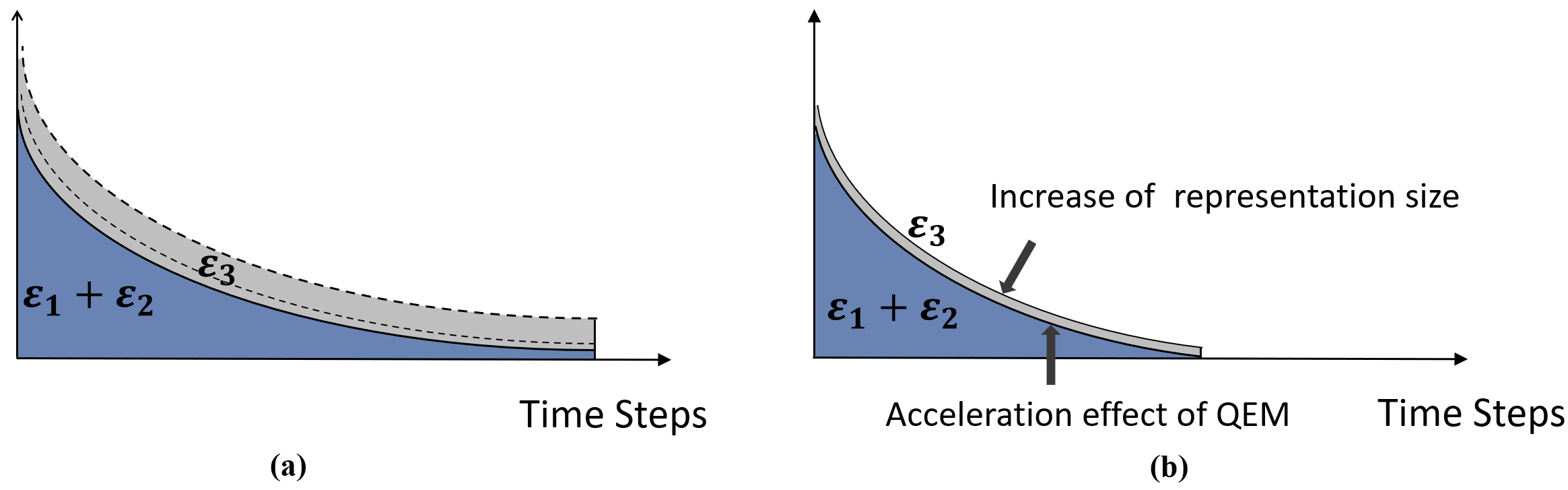
We elaborate on the properties of the three error terms in (1). is derived from the target approximation in quantile loss. is caused by the stochastic approximation of the Bellman operator. results from the parametrization of quantiles and the corresponding projection operator. Among the three, can be theoretically eliminated if the representation size is large enough, whereas is inevitable in practice due to the batch-based optimization procedure. Therefore, controlling the variance can significantly speed up the training convergence (see an illustrating example in Figure 1). Thus, one main target of this work is to reduce the two inevitable errors and , and subsequently improve the existing DRL algorithms.
The contributions of this work are summarized as follows,
-
•
We offer a rigorous investigation on the three error terms , , and in DRL, and find that the approximation errors result from the heteroskedasticity of quantile estimates, especially tail estimates.
-
•
We borrow the idea from the Cornish-Fisher Expansion (Cornish & Fisher, 1938), and propose a statistically robust DRL algorithm, called QEMRL, to reduce the variance of the estimated Q-function.
-
•
We show that QEMRL achieves a higher stability and a faster convergence rate from both theoretical and empirical perspectives.
2 Background
2.1 Reinforcement Learning
Consider a finite Markov Decision Process (MDP) , with a finite set of states , a finite set of actions , the transition kernel , the discounted factor , and the bounded reward function . At each timestep, an agent observes state , takes an action , transfers to the next state , and receives a reward . The state-action value function of a policy is the expected discounted sum of rewards starting from , taking an action and following a policy . denotes the set of probability distributions on a space .
The classic Bellman equation (Bellman, 1966) relates expected return at each state-action pair to the expected returns at possible next states by:
| (2) |
In the learning task, Q-Learning (Watkins, 1989) employs a common way to obtain , which is to find the unique fixed point of the Bellman optimality equation:
2.2 Distributional Reinforcement Learning
Instead of directly estimating the expectation , DRL focuses on estimating the distribution of the sum of discounted rewards to sufficiently capture the intrinsic randomness, where extract the probability distribution of a random variable. In analogy with Equation 2, satisfies the distributional Bellman equation (Bellemare et al., 2017) as follows,
where is defined by and is the pushforward measure of by . Note that is the fixed point of distributional Bellman operator , i.e., .
In general, the return distribution supports a wide range of possible returns and its shape can be quite complex. Moreover, the transition dynamics are usually unknown in practice, and thus the full computation of the distributional Bellman operator is usually either impossible or computationally infeasible. In the following subsections, we review two main categories of DRL algorithms relying on parametric approximations and projection operators.
2.2.1 Categorical distributional RL
Categorical distributional RL (CDRL, Bellemare et al., 2017) represents the return distribution with a categorical form , where denotes the Dirac distribution at . are evenly spaced locations, and are the corresponding probabilities learned using the Bellman update,
where is a categorical projection operator which ensures the return distribution supported only on . In practice, CDRL with has been shown to achieve significant improvement in Atari games.
2.2.2 Quantiled distributional RL
Quantiled distributional RL (QDRL, Dabney et al., 2018b) represents the return distribution with a mixture of Diracs , where are learnable parameters. The Bellman operator moves each atom location towards -th quantile of the target distribution , where . The corresponding Bellman update form is:
where is a quantile projection operator defined by , and is the cumulative distribution function (CDF) of . can be characterized as the minimizer of the quantile regression loss, while the atom locations can be updated by minimizing the following loss function
| (3) |
3 Error Analysis of Distributional RL
As mentioned in Section 1, the parametrization induced error in Section 1 comes from quantile representation and its projection operator, which can be eliminated as . However, as illustrated in Figure 1, the approximation errors and are unavoidable in practice and a high variance may lead to unstable performance of DRL algorithms. Thus, in this section, we further study the three error terms , and , and show why it is important to control them in practice.
3.1 Parametrization Induced Error
We first show the convergence of both the expectation and the variance of the distributional Bellman operator . Then, we take parametric representation and projection operator into consideration.
Proposition 3.1 (Sobel, 1982; Bellemare et al., 2017).
Suppose there are two value distributions , and random variables . Then, we have
Based on the fact that is a -contraction in metric (Bellemare et al., 2017), where is the maximal form of the Wasserstein metric, Proposition 3.1 implies that is a contraction for both the expectation and the variance. The two converge exponentially to their true values by iteratively applying the distributional Bellman operator.
However, in practice, employing parametric representation for the return distribution leaves a theory-practice gap, which makes neither the expectation nor the variance converge to the true values. To better understand the bias in the Q-function approximation caused by the parametric representation, we introduce the concept of mean-preserving 111This property has been thoroughly discussed in previous work. Based on Section 5.11 of Bellemare et al. (2023), we conclude this definition. to describe the relationship between the expectations of the original distribution and the projected distribution:
Definition 3.2 (Mean-preserving).
Let be a projection operator that maps the space of probability distributions to the desired representation. Suppose there is a representation and its associated projection operator are mean-preserving if for any distribution , the expectation of is the same as that of .
For CDRL, a discussion of the mean-preserving property is given by Lyle et al. (2019) and Rowland et al. (2019). It can be shown that for any , where is a -categorical representation, the projection preserves the distribution’s expectation when its support is contained in the interval . However, these practitioners usually employ a wide predefined interval for return which makes the projection operator typically overestimate the variance.
For QDRL, is not mean-preserving (Bellemare et al., 2023). Given any distribution , where is a -quantile representation, there is no unique -quantile distribution in most cases, as the projection operator is not a non-expansion in 1-Wasserstein distance (See Appendix B for details). This means that the expectation, variance, and higher-order moments are not preserved. To make this concrete, a simple MDP example is used to illustrate the bias in the learned quantile estimates.
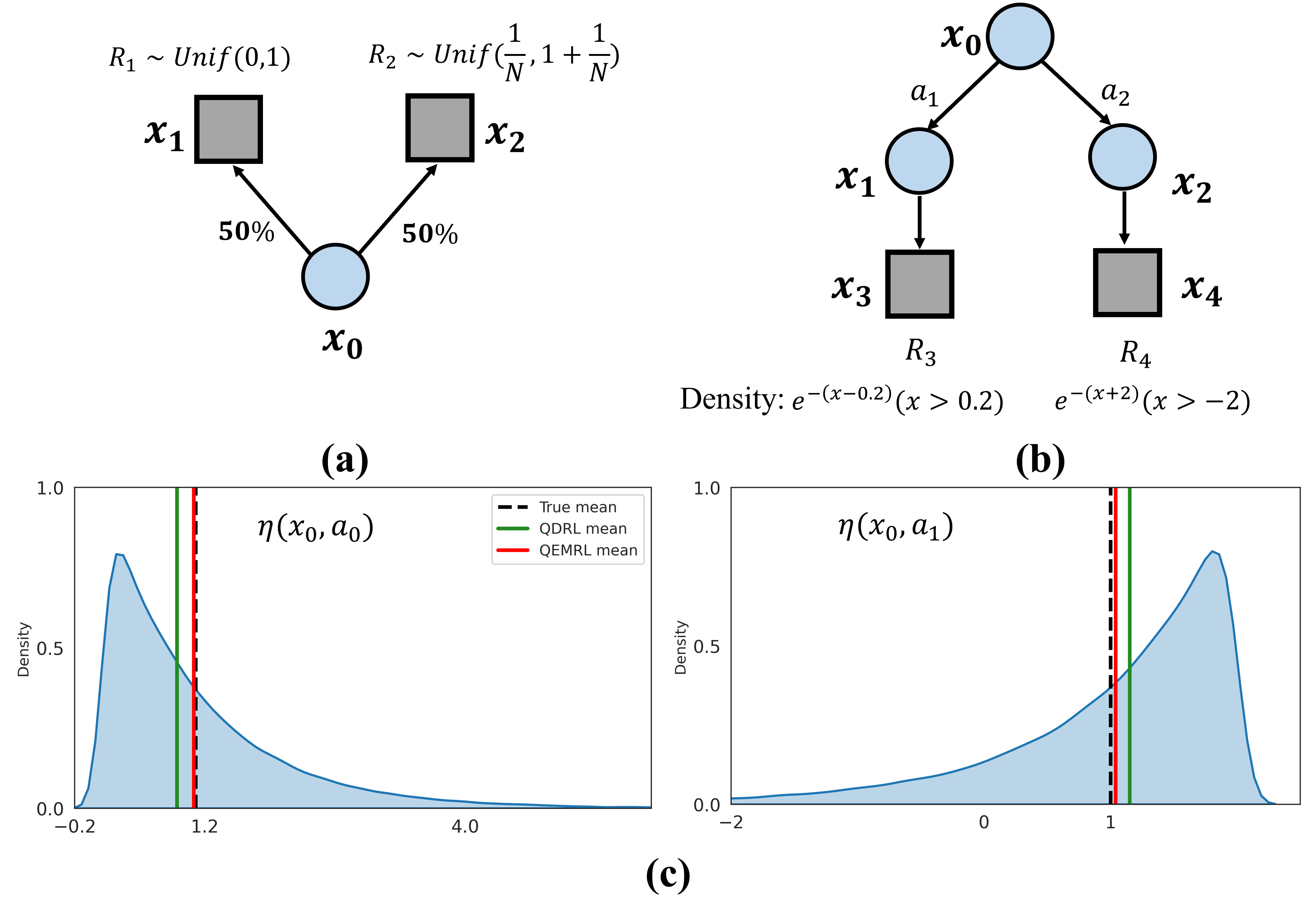
In Figure 2 (a), rewards and are randomly sampled from and at states and respectively, and no rewards are received at . Clearly, the true return distribution at state is the mixture , hence the -th quantile is . When using the QDRL algorithm with quantile estimates, the approximated return distribution and . In this case, the -th quantile of the approximated return distribution at state is , whereas the true value is . Moreover, for each , the -th quantile estimate at state is not equal to the true value.
These biased quantile estimates illustrated in Figure 2 (a) are caused by the use of quantile representation and its projection operator . This undesirable property in turn affects the QDRL update, as the combined operator is in general not a non-expansion in , for (Dabney et al., 2018b), which means that the learned quantile estimates may not converge to the true quantiles of the return distribution 222 A recent study (Rowland et al., 2023a) proves that QDRL update may have multiple fixed points, indicating quantiles may not converge to the truth. Despite this, Proposition 2 (Dabney et al., 2018b) concludes that the projected Bellman operator remains a contraction in . This implies that quantile convergence is guaranteed for all .. The projection operator is not mean-preserving which inevitably leads to bias in the expectation of return distribution when iteratively applying the projected Bellman operator during the training process, resulting in a deviation between the estimate and the true value of the Q-function in the end. We now derive an upper bound to quantify this deviation, i.e. .
Theorem 3.3 (Parameterization induced error bound).
Let be a projection operator onto evenly spaced quantiles ’s where each for , and be the return distribution of -th iteration. Let random variables and . Assume that the distribution of the immediate reward is supported on , then we have
where is parametrization induced error at -th iteration.
Theorem 3.3 implies that the convergence of expectation with projected Bellman operator cannot be guaranteed after quantile representation and its projection operator are applied 333Note that this bound has a limitation, which only considers the one-step effect of applying the projection operator . Therefore, it becomes irrelevant with the iteration number . However, Proposition 4.1 of Rowland et al. (2023b) provides a more compelling bound considering the cumulative effect of iteratively applying .. Note that the bound will tend to zero with , thus it is reasonable to use a relatively large representation size to reduct in practice.
3.2 Approximation Error
The other two types of errors and , which determine the variance of the Q-function estimate, are accumulated during the training process by keeping encountering unseen state-action pairs. The target approximation error affects action selections, while the Bellman operator approximation error leads to the accumulated error of the Q-function estimate, which can be amplified by using the temporal difference updates (Sutton, 1988). The accumulated errors of the Q-function estimate with high uncertainty can make some certain states to be incorrectly estimated, leading to suboptimal policies and potentially divergent behaviors.
As depicted in Figure 2 (b), we utilize this toy example to illustrate how QDRL fails to learn an optimal policy due to a high variance of the approximation error. This 5-state MDP example is originally introduced in Figure 7 of Rowland et al. (2019). In this case, and follow exponential distributions, and the expectations of them are 1.2 and 1, respectively. We consider a tabular setting, which uniquely represents the approximated return distribution at each state-action pair. Figure 2 (c) demonstrates that in policy evaluation, QDRL inaccurately approximates the Q-function, as it underestimates the expectation of and overestimates the other. This is caused by the poor capture of tail events, which results in high uncertainty in the Q-function estimate. Due to the high variance, QDRL fails to learn the optimal policy and chooses a non-optimal action at the initial state . On the contrary, our proposed algorithm, QEMRL, employs a statistically robust estimator of the Q-function to reduce its variance, relieves the underestimation and overestimation issues, and ultimately allows for more efficient policy learning.
Different from previous QDRL studies that focus on exploiting the distribution information to further improve the model performance, this work highlights the importance of controlling the variance of the approximation error to obtain a more accurate estimate of the Q-function. More discussion about this is given in the following section.
4 Quantiled Expansion Mean
This section introduces a novel variance reduction technique to estimate the Q-function. In traditional statistics, estimators with lower variance are considered to be more efficient. In RL, variance reduction is also an effective technique for achieving fast convergence in both policy-based and value-based RL algorithms, especially for large-scale tasks (Greensmith et al., 2004; Anschel et al., 2017). Motivated by these findings, we introduce QEM as an estimator that is more robust and has a lower variance than that of QDRL under the heteroskedasticity assumption. Furthermore, we demonstrate the potential benefits of QEM for the distribution approximation in DRL.
4.1 Heteroskedasticity of quantiles
In the context of quantile-based DRL, Q-function is the integral of the quantiles. To approximate this, QDRL employs a simple empirical mean (EM) estimator , and it is natural to assume that the estimated quantile satisfies
| (4) |
where is a zero-mean error. In this case, considering the crossing issue and the biased tail estimates, we assume that the variance of is non-constant and depends on , which is usually called heteroskedasticity in statistics.
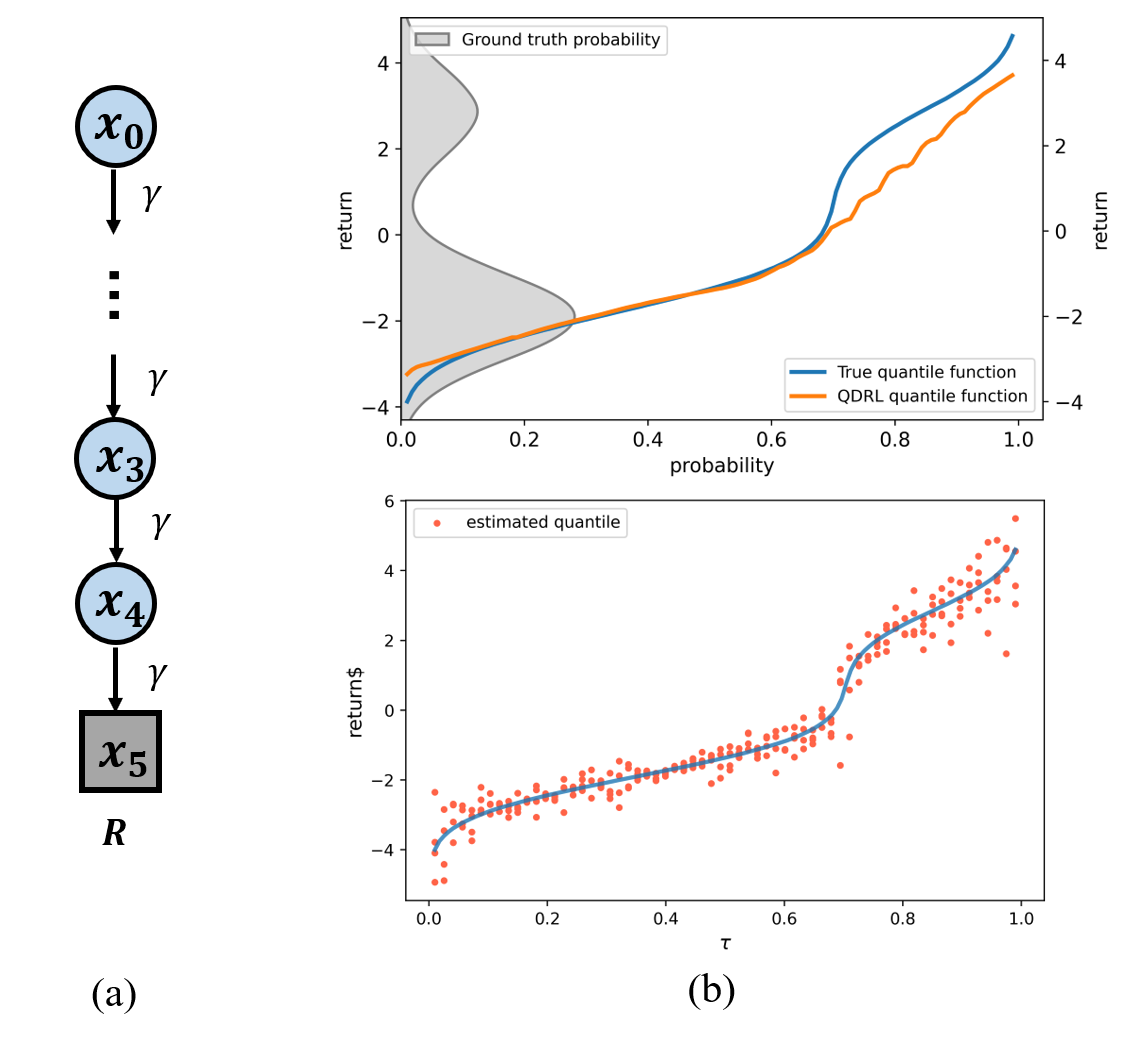
For a direct understanding, we conduct a simple simulation using a Chain MDP to illustrate how QDRL can fail to fit the quantile function. As shown in Figure 3(b), QDRL fits well in the peak area but struggles at the bottom and the tail. Moreover, the non-monotonicity of the quantile estimates in the poorly fitted areas is more severe than the others. As the deviations of the quantile estimates from the truths is significantly larger in the low probability region and the tail, we can make the heteroskedasticity assumption in this case. This phenomenon can be explained since samples near the bottom and the tail are less likely to be drawn. In real-world situations, multimodal distributions are commonly encountered and the heteroskedasticity problem may result in imprecise distribution approximations and consequently poor Q-function approximations. In the next part, we will discuss how to enhance the stability of the Q-function estimate.
4.2 Cornish-Fisher Expansion
It is well-known that quantile can be expressed by the Cornish-Fisher Expansion (CFE, Cornish & Fisher, 1938):
| (5) | ||||
where is the -th quantile of the standard normal distribution, is the mean, is the standard deviation, and are the skewness and kurtosis of the interested distribution, and the remaining terms in the ellipsis are higher-order moments (See Appendix C for more details). The CFE theoretically determines the distribution with known moments and is widely used in financial studies. Recently, Zhang & Zhu (2023) employ CFE to estimate higher-order moments of financial time series data, which are not directly observable. Our method utilizes a truncated version of CFE framework and employs a linear regression model to construct efficient estimators for distribution moments based on known quantiles. Consequently, we apply this approach within the context of quantile-based DRL.
To be more specific, we plug in the estimate of the the -th quantile to Equation 5 and expand it by the first order:
| (6) |
where is the mean (say, -th moment) of the return distribution, i.e., the Q-function, and is the remaining term associated with the higher-order (-th) moments. If is negligible, can be estimated by averaging the quantile estimates in QDRL.
When the estimated quantile is expanded to the second order, we particularly have the following representation:
| (7) |
where is the remaining term associated with the higher-order (-th) moments. Assume that is negligible, we can derive a regression model by plugging in the quantile estimates, such that
| (22) |
The higher-order expansions can be conducted in the same manner. Note that the remaining term is omitted for constructing a regression model, and a more in-depth analysis of the remaining term is available in Section C.2.
For notation simplicity, we rewrite (22) in a matrix form,
| (23) |
where is the vector of estimated quantiles, and are the design matrix and the moments respectively, and is the vector of error terms.
For this bivariate regression model (23), the traditional ordinary least squares method (OLS) can be used to estimate when the variances of the errors are invariant across different quantile locations, also known as the homoscedasticity assumption. The estimator is denoted as Quantiled Expansion Mean (QEM) in this work. However, since the homoscedasticity assumption required by OLS is always violated in real cases, we may consider using the weighted ordinary least squares method (WLS) instead. Under the normality assumption, the following results tell that the WLS estimator has a lower variance than the direct empirical mean.
Lemma 4.1.
Consider the linear regression model , is distributed on , where , and we set noise variance without loss of generality. The WLS estimator is
| (24) |
and the QEM estimator is the first component of .
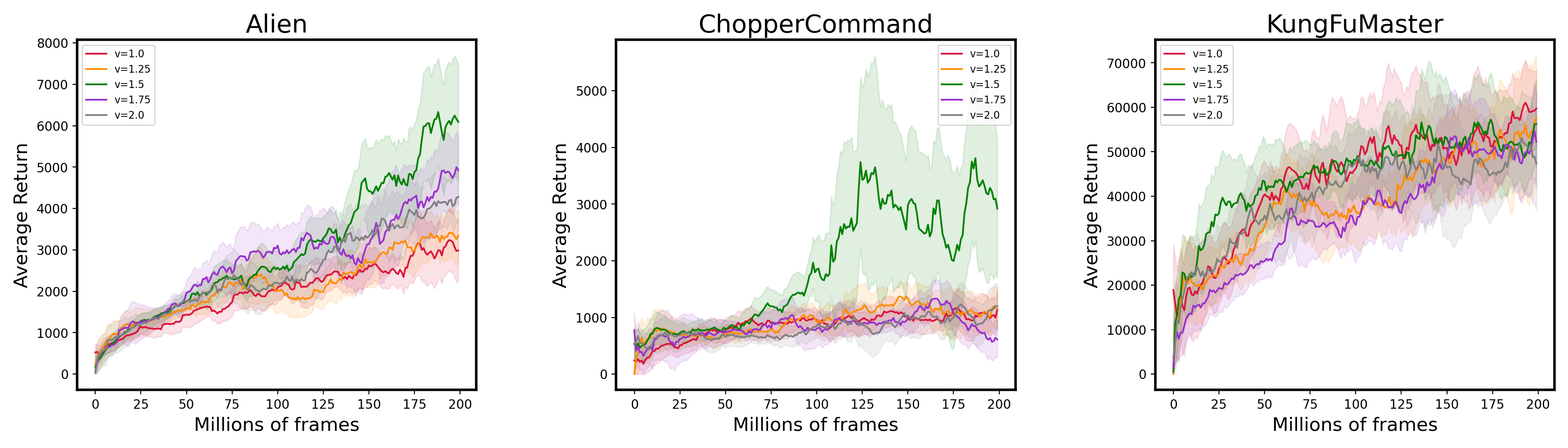
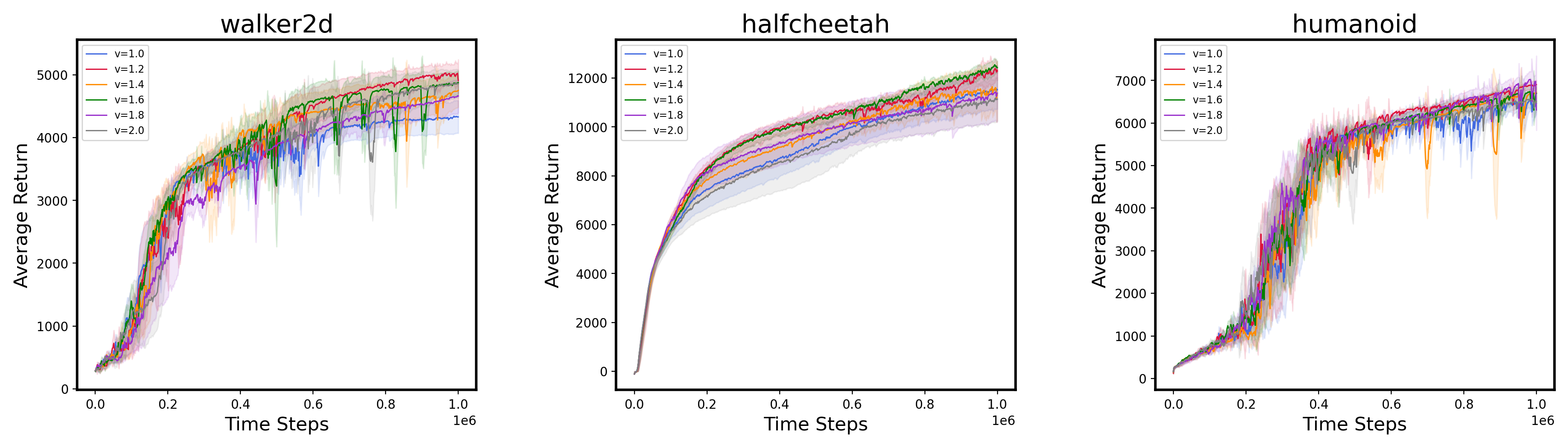
Remark: Note that it is impossible to determine the weight matrix for each state-action pair in practice. Hence, we focus on capturing the relatively high variance in the tail, specifically in the range of . To achieve this, we use a constant , which is set to a value greater than 1 in the tail and equal to 1 in the rest. is treated as a hyperparameter to be tuned in practice (See Appendix E).
With Lemma 4.1, the reduction of variance can be guaranteed by the following Proposition 4.2. Throughout the training process, heteroskedasticity is inevitable, and thus the QEM estimator always exhibits a lower variance than the standard EM estimator .
Proposition 4.2.
Suppose the noise independently follows where for , then,
(i) In the homoskedastic case where for , the empirical mean estimator has a lower variance, ;
(ii) In the heteroskedastic case where ’s are not eaqul, the QEM estimator achieves a lower variance, i.e. , if and only if , where . This inequality holds when , which can be guaranteed in QDRL.
We also try to explore the potential benefits of the variance reduction technique QEM in improving the approximation accuracy. The Q-function estimate with higher variance can lead to noisy policy gradients in policy-based algorithms (Fujimoto et al., 2018) and prevent selection optimal actions in value-based algorithms (Anschel et al., 2017). These issues can slow down the learning process and negatively impact the algorithm performance. By the following theorem, we are able to show that QEM can reduce the variance and thus improve the approximation performance.
Theorem 4.3.
Consider the policy that is learned policy, and denote the optimal policy to be , , and . For all , with probability at least , for any , and all ,
Theorem 4.3 indicates that a lower concentration bound can be obtained with a smaller value. The decrease in can be attributed to the benefits of QEM. Specifically, QEM helps to decrease the perturbations on the Q-function and reduce the variance of the policy gradients, which allows for faster convergence of the policy training and a more accurate distribution approximation. To conclude, QEM relieves the error accumulation within the Q-function update, improves the estimation accuracy, reduces the risk of underestimation and overestimation, and thus ultimately enhances the stability of the whole training process.
5 Experimental Results
In this section, we do some empirical studies to demonstrate the advantage of our QEMRL method. First, a simple tabular experiment is conducted to validate some of the theoretical results presented in Sections 3 and 4. Then we apply the proposed QEMRL update strategy in Algorithm 1 to both the DQN-style and SAC-style DRL algorithms, which are evaluated on the Atari and MuJoCo environments. The detailed architectures of these methods and the hyperparameter selections can be found in Appendix D, and the additional experimental results are included in Appendix E.
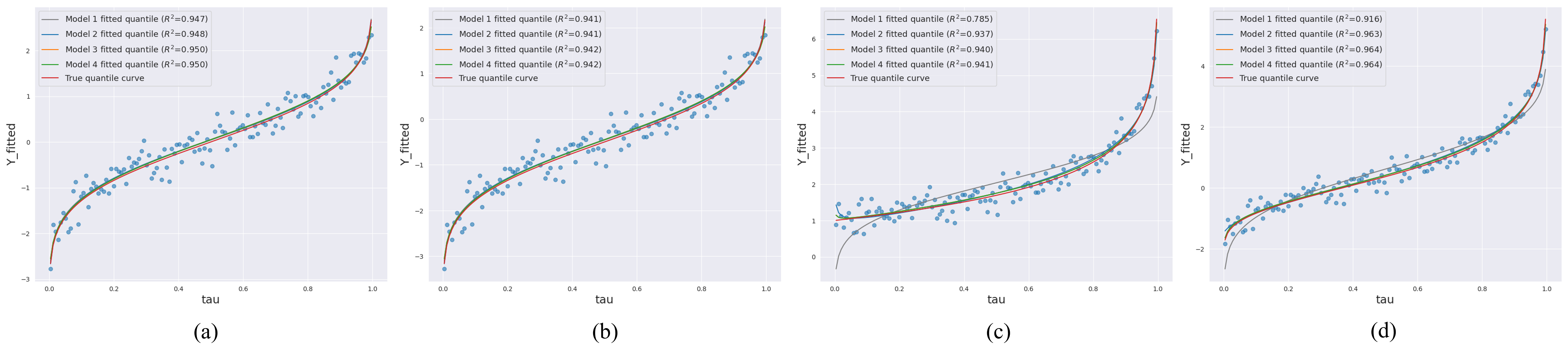
In this work, we implement QEM using a -th order expansion that includes mean, variance, skewness, and kurtosis in this work. The effects of a higher-order expansion on model estimation are discussed in Section C.1. Intuitively, including more terms in the expansion improves the estimation accuracy of quantiles, but the overfitting risk and the computational cost are also increased. Hence, there is a trade-off between explainability and learning efficiency. We evaluate different expansion orders using the statistic, which measures the goodness of model fitting. The simulation results (Figure 9) show that a -th order expansion seems to be the optimal choice while a higher-order (-th) expansion does not show a significant increase in .
5.1 A Tabular Example
FrozenLake (Brockman et al., 2016) is a classic benchmark problem for Q-learning control with high stochasticity and sparse rewards, in which an agent controls the movement of a character in an grid world. As shown in Figure 4 with a FrozenLake- task, ”S” is the starting point, ”H” is the hole that terminates the game, ”G” is the goal state with a reward of 1. All the blue grids stand for the frozen surface where the agent can slide to adjacent grids based on some underlying unknown probabilities when taking a certain movement direction. The reward received by the agent is always zero unless the goal state is reached.
We first approximate the return distribution under the optimal policy , which can be realized using the value iteration approach. To be specific, we start from the ”S” state and perform 1K Monte-Carlo (MC) rollouts. An empirical distribution can be obtained by summarizing all these recording trajectories. With the approximation of the distribution, we can draw a curve of quantile estimates shown in Figure 5. Both QEMRL and QDRL were run for 150K training steps and the -greedy exploration strategy is applied in the first 1K steps. For both methods, we set the total number of quantiles to be .
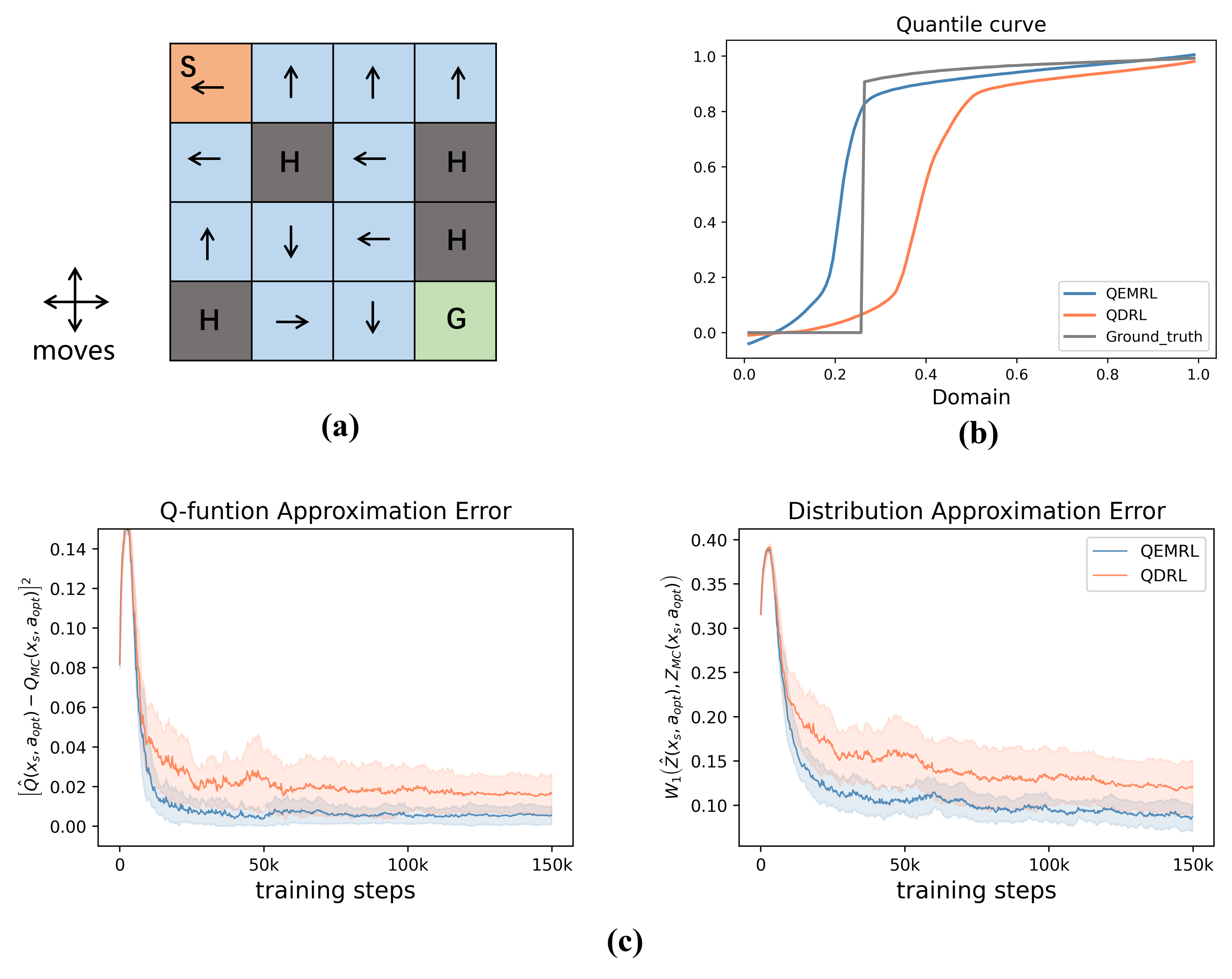
Although both QEMRL and QDRL can eventually find the optimal movement at the start state, their approximations of the return distribution are quite different. Figure 4 (b) visualizes the approximation errors of the Q-function and the distribution for QEMRL and QDRL with respect to the number of training steps. The Q-function estimates of QEMRL converge correctly in average, whereas the estimates of QDRL do not converge exactly to the truth. A similar pattern can also be found when it comes to the distribution approximation error. Besides, the reduction of variance by using QEM can be verified by the fact that the curves of QEMRL are more stable and decline faster. In Figure 4 (c), we show that the distribution at the start state estimated by QEMRL is eventually closer to the ground truth.
5.2 Evaluation on MuJoCo and Atari 2600
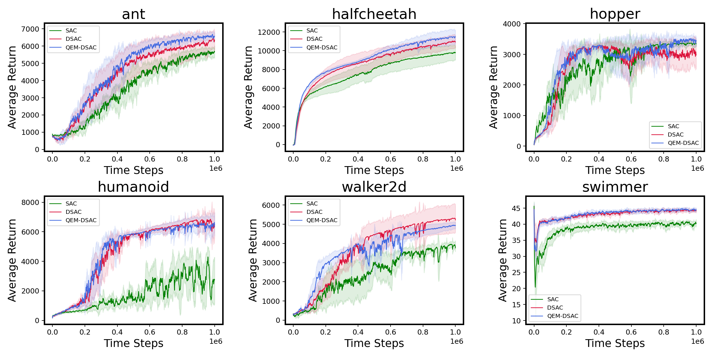
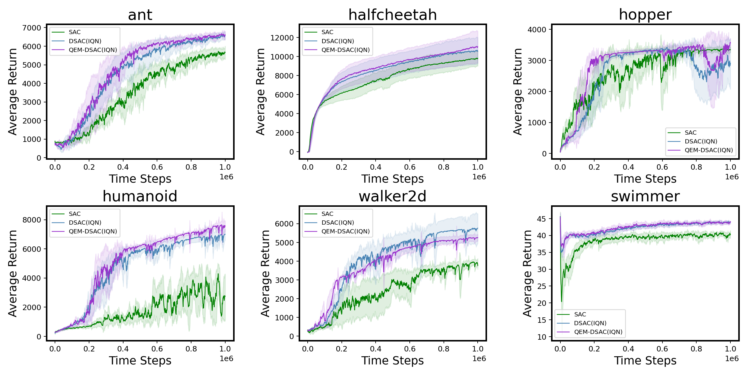
We do some experiments using the MuJoCo benchmark to further verify the analysis results in Section 4. Our implementation is based on the Distributional Soft Actor-Critic (DSAC, Ma et al., 2020) algorithm, which is a distributional version of SAC. Figure 5 demonstrate that both DSAC and QEM-DSAC significantly outperform the baseline SAC. Among the two, QEM-DSAC performs better than DSAC and the learning curves are more stable, which demonstrates that QEM-DSAC can achieve a higher sample efficiency.
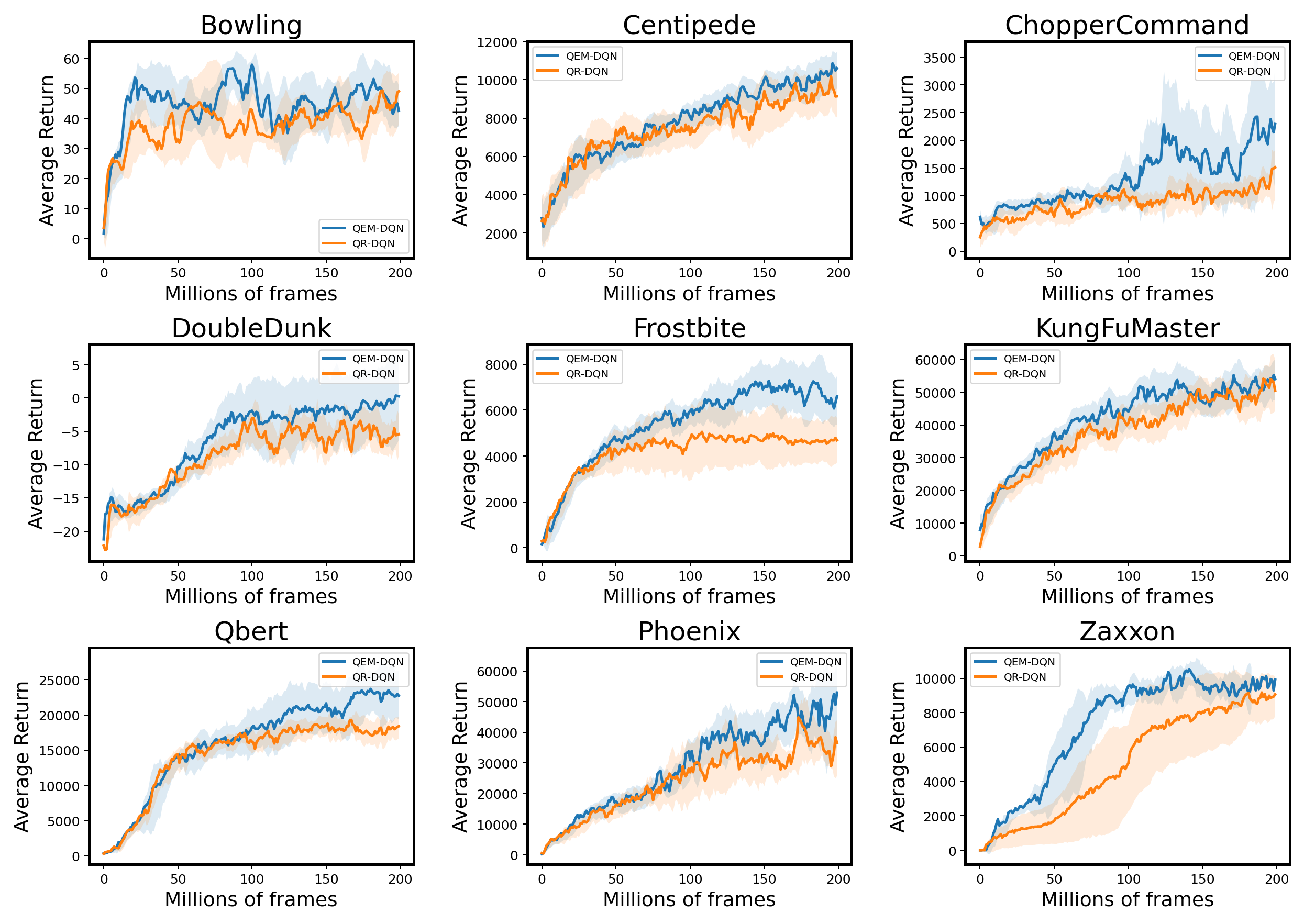
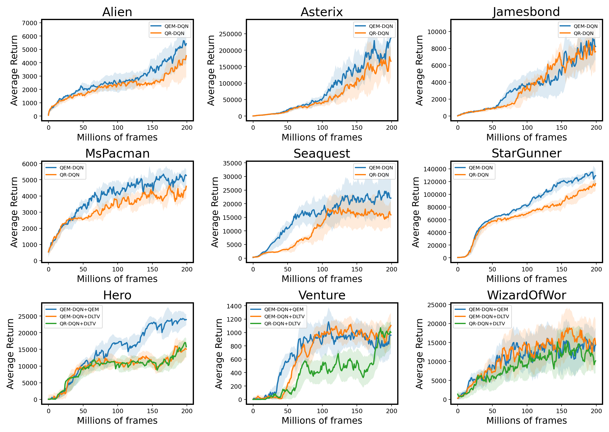
We also do some comparison between QEM and the baseline method QR-DQN on the Atari 2600 platform. Figure 8 plots the final results of these two algorithms in six Atari games. At the early training stage, QEM-DQN exhibits significant gain in sampling efficiency, resulting in faster convergence and better performance.
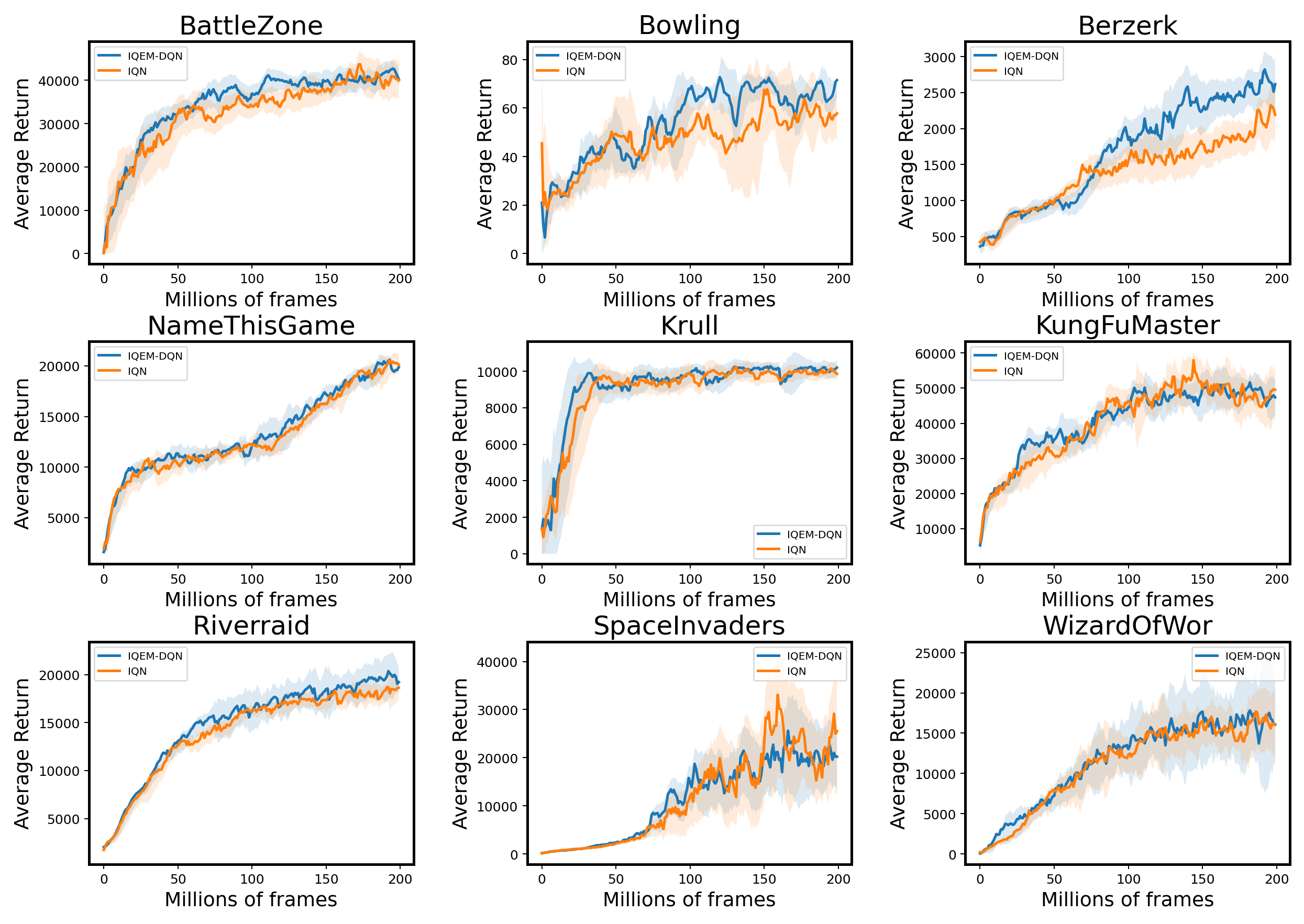
Extension to IQN. Some great efforts have been made by the community of DRL to more precisely parameterize the entire distribution with a limited number of quantile locations. One notable example is the introduction of Implicit Quantile Networks (IQN, Dabney et al., 2018a), which tries to recover the continuous map of the entire quantile curve by sampling a different set of quantile values from a uniform distribution each time.
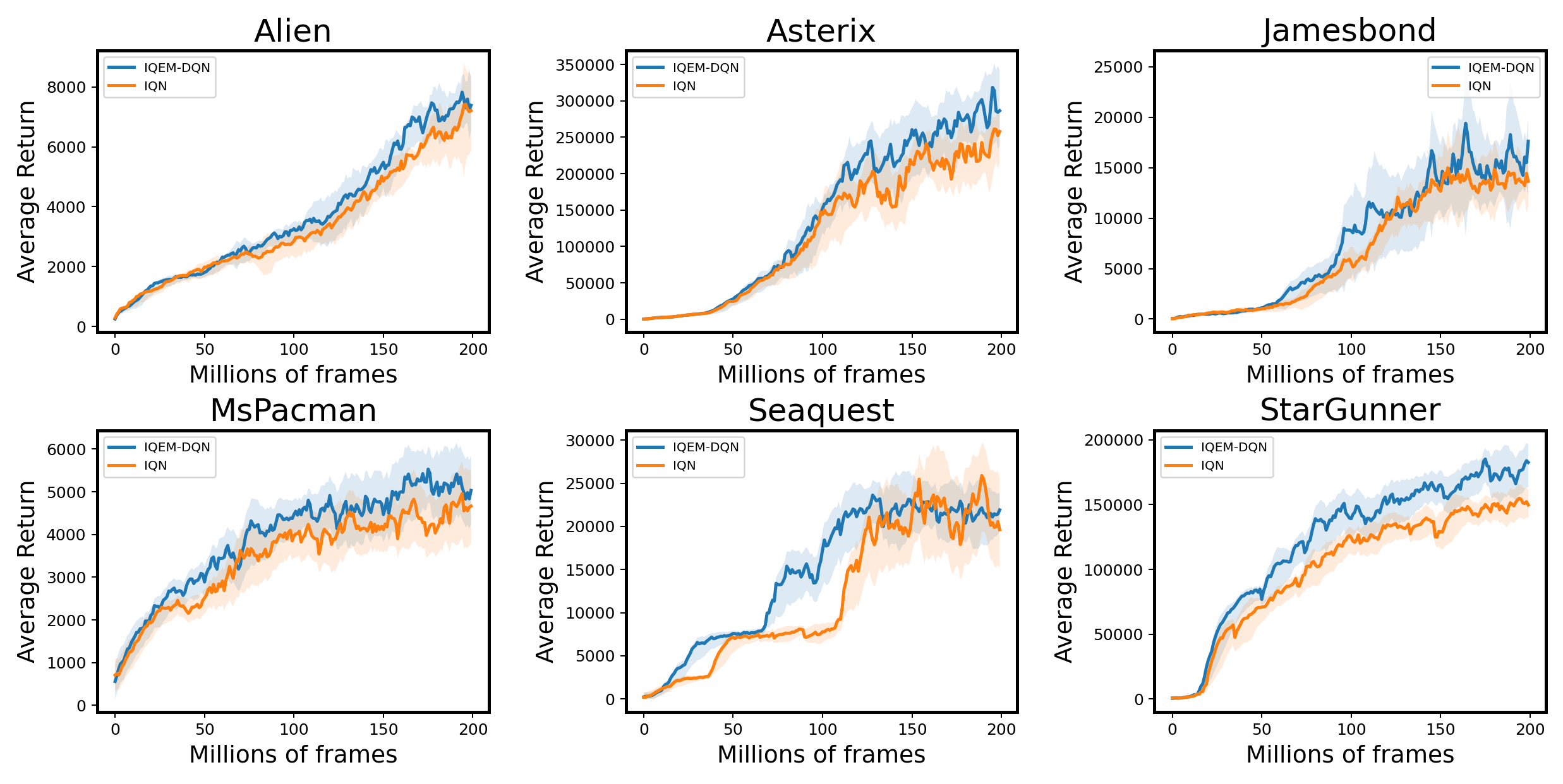
Our method can also be applied to IQN as it uses the EM approach to estimate the Q-function. It is noted that the design matrix must be updated after re-sampling all the quantile fractions at each training step. Moreover, one important sufficient condition which ensures the reduction of variance does not hold in the IQN case as ’s are sampled from a uniform distribution. However, according to the simulation results in LABEL:table4, the variance reduction still remains valid in practice. In this case, all the baseline methods are modified to the IQN version. As Figure 6 and Figure 7 demonstrate, QEM can achieve some performance gain in most scenarios and the convergence speeds can be slightly increased.
5.3 Exploration
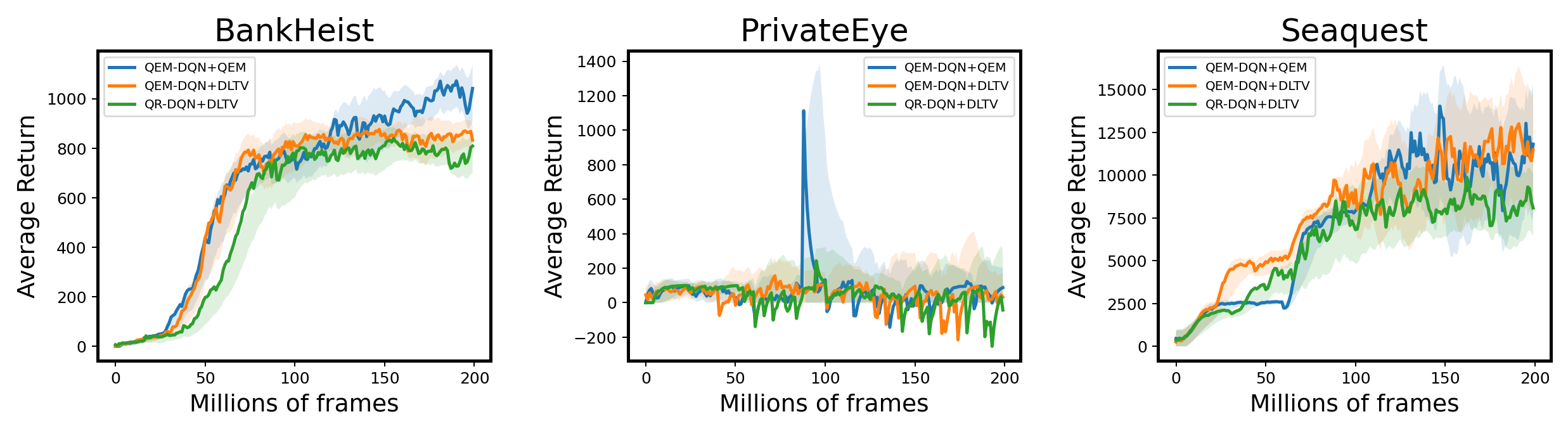
Since QEM also provides an estimate of the variance, we may consider using it to develop an efficient exploration strategy. In some recent study studies, to more sufficiently utilize the distribution information, Mavrin et al. (2019) proposes a novel exploration strategy, Decaying Left Truncated Variance (DLTV) by using the left truncated variance of the estimated distribution as a bonus term to encourage exploration in unknown states. The optimal action at state is selected according to , where is a decay factor to suppress the intrinsic uncertainty, and denotes the estimation of variance. Although DLTV is effective, the validity of the computed truncation lacks a theoretical guarantee. In this work, we follow the idea of DLTV and examine the model performance by using either the variance estimate obtained by QEM or the original DLTV estimation in some hard-explored games. As Figure 8 shows, by using QEM, the exploration efficiency is significantly improved compared to QR-DQN+DLTV since QEM enhances the accuracy of the quantile estimates and thus the accuracy of the distribution variance.
6 Conclusion and Discussion
In this work, we systematically study the three error terms associated with the Q-function estimate and propose a novel DRL algorithm QEMRL, which can be applied to any quantile-based DRL algorithm regardless of whether the quantile locations are fixed or not. We found that a more robust estimate of the Q-function can improve the distribution approximation and speed up the algorithm convergence. We can also utilize the more precise estimate of the distribution variance to optimize the existing exploration strategy.
Finally, there are some open questions we would like to have further discussions here.
Improving the estimation of weight matrix . The challenge of estimating the weight matrix was recognized from the outset of the method proposal since it is unlikely to know the exact value of in practice. In this work, we treat as a predefined value that can be tuned, taking into account the computational cost of estimating it across all state-action pairs and time steps. As for future work, we believe a robust and easy-to-implement estimation of weight matrix is necessary. Given that the variance of quantile estimation errors varies with state-action pairs and algorithm iterations, we consider two approaches for future investigation. The first approach considers a decay value of instead of the constant. It is worth noting that the variance of poorly estimated quantiles tends to decrease gradually as the number of training samples increases, which motivates us to decrease the value of as training epochs increase. The second approach involves assigning different values of to different state-action pairs. Ideas from the exploration field, specifically the count-based method (Ostrovski et al., 2017), can be borrowed to measure the novelty of state-action pairs. Accordingly, for familiar state-action pairs, a smaller value of should be assigned, while unfamiliar pairs should be assigned a larger value of .
Statistical variance reduction. Our variance reduction method is based on a statistical modeling perspective, and the core insight of our method is that performance might be improved through more careful use of the quantiles to construct a Q-function estimator. While alternative ensembling methods can be directly applied to DRL to reduce the uncertainty in Q-function estimator, commonly used in existing works (Osband et al., 2016; Anschel et al., 2017), it undoubtedly increases model complexity. In this work, we transform the Q value estimation into a linear regression problem, where the Q value is the coefficient of the regression model. In this way, we can leverage the weighted least squares (WLS) method to effectively capture the heteroscedasticity of quantiles and obtain a more efficient and robust Q-function estimator.
Acknowledgements
We thank anonymous reviewers for valuable and constructive feedback on an early version of this manuscript. This work is supported by National Social Science Foundation of China (Grant No.22BTJ031 ) and Postgraduate Innovation Foundation of SUFE. Dr. Fan Zhou’s work is supported by National Natural Science Foundation of China (12001356), Shanghai Sailing Program (20YF1412300), “Chenguang Program” supported by Shanghai Education Development Foundation and Shanghai Municipal Education Commission, Open Research Projects of Zhejiang Lab (NO.2022RC0AB06), Shanghai Research Center for Data Science and Decision Technology, Innovative Research Team of Shanghai University of Finance and Economics.
References
- Anschel et al. (2017) Anschel, O., Baram, N., and Shimkin, N. Averaged-dqn: Variance reduction and stabilization for deep reinforcement learning. In International Conference on Machine Learning, pp. 176–185. PMLR, 2017.
- Bellemare et al. (2017) Bellemare, M. G., Dabney, W., and Munos, R. A distributional perspective on reinforcement learning. In International Conference on Machine Learning, pp. 449–458. PMLR, 2017.
- Bellemare et al. (2023) Bellemare, M. G., Dabney, W., and Rowland, M. Distributional Reinforcement Learning. MIT Press, 2023. http://www.distributional-rl.org.
- Bellman (1966) Bellman, R. Dynamic programming. Science, 153(3731):34–37, 1966.
- Brockman et al. (2016) Brockman, G., Cheung, V., Pettersson, L., Schneider, J., Schulman, J., Tang, J., and Zaremba, W. Openai gym. arXiv preprint arXiv:1606.01540, 2016.
- Cornish & Fisher (1938) Cornish, E. A. and Fisher, R. A. Moments and cumulants in the specification of distributions. Revue de l’Institut international de Statistique, pp. 307–320, 1938.
- Dabney et al. (2018a) Dabney, W., Ostrovski, G., Silver, D., and Munos, R. Implicit quantile networks for distributional reinforcement learning. In International Conference on Machine Learning, pp. 1096–1105, 2018a.
- Dabney et al. (2018b) Dabney, W., Rowland, M., Bellemare, M. G., and Munos, R. Distributional reinforcement learning with quantile regression. In Proceedings of the AAAI Conference on Artificial Intelligence, 2018b.
- Fujimoto et al. (2018) Fujimoto, S., Hoof, H., and Meger, D. Addressing function approximation error in actor-critic methods. In International Conference on Machine Learning, pp. 1587–1596. PMLR, 2018.
- Greensmith et al. (2004) Greensmith, E., Bartlett, P. L., and Baxter, J. Variance reduction techniques for gradient estimates in reinforcement learning. Journal of Machine Learning Research, 5(9), 2004.
- Hsu et al. (2011) Hsu, D., Kakade, S. M., and Zhang, T. An analysis of random design linear regression. arXiv preprint arXiv:1106.2363, 2011.
- Koenker (2005) Koenker. Quantile regression. Cambridge University Press, 2005.
- Kuznetsov et al. (2020) Kuznetsov, A., Shvechikov, P., Grishin, A., and Vetrov, D. Controlling overestimation bias with truncated mixture of continuous distributional quantile critics. In International Conference on Machine Learning, pp. 5556–5566. PMLR, 2020.
- Luo et al. (2021) Luo, Y., Liu, G., Duan, H., Schulte, O., and Poupart, P. Distributional reinforcement learning with monotonic splines. In International Conference on Learning Representations, 2021.
- Lyle et al. (2019) Lyle, C., Bellemare, M. G., and Castro, P. S. A comparative analysis of expected and distributional reinforcement learning. In Proceedings of the AAAI Conference on Artificial Intelligence, volume 33, pp. 4504–4511, 2019.
- Ma et al. (2020) Ma, X., Xia, L., Zhou, Z., Yang, J., and Zhao, Q. Dsac: distributional soft actor critic for risk-sensitive reinforcement learning. arXiv preprint arXiv:2004.14547, 2020.
- Mavrin et al. (2019) Mavrin, B., Yao, H., Kong, L., Wu, K., and Yu, Y. Distributional reinforcement learning for efficient exploration. In International Conference on Machine Learning, pp. 4424–4434, 2019.
- Nguyen-Tang et al. (2021) Nguyen-Tang, T., Gupta, S., and Venkatesh, S. Distributional reinforcement learning via moment matching. In Proceedings of the AAAI Conference on Artificial Intelligence, volume 35, pp. 9144–9152, 2021.
- Osband et al. (2016) Osband, I., Blundell, C., Pritzel, A., and Van Roy, B. Deep exploration via bootstrapped dqn. Advances in Neural Information Processing Systems, 29, 2016.
- Ostrovski et al. (2017) Ostrovski, G., Bellemare, M. G., Oord, A., and Munos, R. Count-based exploration with neural density models. In International Conference on Machine Learning, pp. 2721–2730. PMLR, 2017.
- Rowland et al. (2018) Rowland, M., Bellemare, M., Dabney, W., Munos, R., and Teh, Y. W. An analysis of categorical distributional reinforcement learning. In International Conference on Artificial Intelligence and Statistics, pp. 29–37. PMLR, 2018.
- Rowland et al. (2019) Rowland, M., Dadashi, R., Kumar, S., Munos, R., Bellemare, M. G., and Dabney, W. Statistics and samples in distributional reinforcement learning. In International Conference on Machine Learning, pp. 5528–5536. PMLR, 2019.
- Rowland et al. (2023a) Rowland, M., Munos, R., Azar, M. G., Tang, Y., Ostrovski, G., Harutyunyan, A., Tuyls, K., Bellemare, M. G., and Dabney, W. An analysis of quantile temporal-difference learning. arXiv preprint arXiv:2301.04462, 2023a.
- Rowland et al. (2023b) Rowland, M., Tang, Y., Lyle, C., Munos, R., Bellemare, M. G., and Dabney, W. The statistical benefits of quantile temporal-difference learning for value estimation. arXiv preprint arXiv:2305.18388, 2023b.
- Sobel (1982) Sobel, M. J. The variance of discounted markov decision processes. Journal of Applied Probability, 19(4):794–802, 1982.
- Sutton (1988) Sutton, R. S. Learning to predict by the methods of temporal differences. Machine Learning, 3:9–44, 1988.
- Villani (2009) Villani, C. Optimal transport: old and new, volume 338. Springer, 2009.
- Watkins (1989) Watkins, C. J. C. H. Learning from delayed rewards. PhD thesis, 1989.
- Yang et al. (2019) Yang, D., Zhao, L., Lin, Z., Qin, T., Bian, J., and Liu, T.-Y. Fully parameterized quantile function for distributional reinforcement learning. In Advances in Neural Information Processing Systems, pp. 6193–6202, 2019.
- Zhang & Zhu (2023) Zhang, N. and Zhu, K. Quantiled conditional variance, skewness, and kurtosis by cornish-fisher expansion. arXiv preprint arXiv:2302.06799, 2023.
- Zhou et al. (2020) Zhou, F., Wang, J., and Feng, X. Non-crossing quantile regression for distributional reinforcement learning. Advances in Neural Information Processing Systems, 33:15909–15919, 2020.
- Zhou et al. (2021) Zhou, F., Zhu, Z., Kuang, Q., and Zhang, L. Non-decreasing quantile function network with efficient exploration for distributional reinforcement learning. International Joint Conference on Artificial Intelligence, pp. 3455–3461, 2021.
Appendix A Projection Operator
A.1 Categorical projection operator
CDRL algorithm uses a categorical projection operator to restrict approximated distributions to the parametric family of the form , where are evenly spaced, fixed supports. The operator is defined for a single Dirac delta as
A.2 Quantile projection operator
QDRL algorithm uses a quantile projection operator to restrict approximated distributions to the parametric family of the form . The operator is defined as
where , and is the CDF of . The midpoint of the interval minimizes the 1-Wasserstein distance between the distribution, , and its projection (a -quantile distribution with evenly spaced ), as demonstrated in Lemma 2 (Dabney et al., 2018b).
Appendix B Proofs
In this section, we provide the proofs of the theorems discussed in the main manuscript.
B.1 Proof of Section 3
Proposition B.1 (Sobel, 1982; Bellemare et al., 2017).
Suppose there are value distributions , and random variables . Then, we have
Proof.
This proof follows directly from Bellemare et al. (2017). The first statement can be proved using the exchange of . By independence of and , where is the transition operator, we have
Thus, we have
∎
Lemma B.2 (Lemma B.2 of Rowland et al. (2019)).
Let , for . Consider the corresponding 1-Wasserstein projection operator , defined by
for all , where is the inverse CDF of . Let random variable , , and . Suppose immediate reward distributions supported on . Then, we have:
(i) ;
(ii) ;
(iii) .
Proof.
This proof follows directly from Lemma B.2 of Rowland et al. (2019). For proving (i), let be the inverse CDF of . We have
For proving (ii), using the triangle inequality and statement (i):
(ii) implies the fact that the quantile projection operator is not a non-expansion under 1-Wasserstein distance, which is important for the uniqueness of the fixed point and the convergence of the algorithm.
The proof of (iii) is similar to (i), using the fact that the return distribution is bounded on to obtain the following inequality:
∎
Theorem B.3 (Parameterization induced error bound).
Let be a projection operator onto evenly spaced quantiles ’s where each for , and be the return distribution of -th iteration. Let random variables and . Assume that the distribution of the immediate reward is supported on , then we have
where is parametrization induced error at -th iteration.
Proof.
Using the dual representation of the Wasserstein distance (Villani, 2009) and Lemma B.2, , we have
By taking the limitation over and iteration on the left-hand side, we obtain
In a similar way, the second-order moment can be bounded by,
It suggests that higher-order moments are not preserved after quantile representation is applied. ∎
B.2 Proof of Section 4
Lemma B.4 (expectation by quantiles).
. Let be a random variable with CDF and quantile function . Then,
Proof.
As any CDF is non-decreasing and right continuous, we have for all :
Then, denoting by a uniformly distributed random variable over ,
which shows that the random variable has the same distribution as . Hence,
∎
Lemma B.5.
Consider the linear regression model , is distributed on , where , and we set noise variance without loss of generality. The WLS estimator is
| (25) |
and the distribution of mean estimator takes the form,
When equals identity matrix ,
Proof.
Premultiplying by , we get the transformed model
Now, set , and , so that the transformed model can be written as . The transformed model is a Gaussian-Markov model, satisfying OLS assumptions. Thus, the unique OLS solution is and By computing we derive ∎
Proposition B.6.
Suppose the noise independently follows where for , then,
(i) In the homoskedastic case where for , the empirical mean estimator has a lower variance, ;
(ii) In the heteroskedastic case where ’s are not equal, the QEM estimator achieves a lower variance, i.e. , if and only if , where . This inequality holds when , which can be guaranteed in QDRL.
Proof.
The proof of (i) comes directly from the comparison of variances, i.e. . Next, we prove that (ii) holds under a sufficient condition . In QDRL, the quantile levels are equally spaced around 0.5. Under this setup, the condition indeed holds, where is the -th quantile of standard normal distribution. For , we need to validate the inequality . This can be transformed into a multivariate extreme value problem. By analyzing the function , the infimum of is 0 when , and reaches 0 at the limit . For , this case is identical to since . For , , and this expression can be factored as, , where , and . By comparing the coefficient corresponding to the same terms, we can verify that when . Finally, the remaining cases can be proven in the same manner.
∎
Theorem B.7.
Consider the policy that is learned policy, and denote the optimal policy to be , , and . For all , with probability at least , for any , and all ,
Proof.
We give this proof in a tabular MDP. Directly following from the definition of the distributional Bellman operator applied to the CDF, we have that
For notation convenience, we use random variables instead of measures. and are the maximum likelihood estimates of the transition and the reward functions, respectively. Adding and subtracting , then we have
For the first term, note that
(a) follows from the fact that , and
The second term can be bounded as follows:
Next, we show the two norms can be bounded. By the Dvoretzky-Kiefer-Wolfowitz (DKW) inequality, the following inequality holds with probability at least , for all ,
By Hoeffding’s inequality and an concentration bound for multinomial distribution444 see https://nanjiang.cs.illinois.edu/files/cs598/note3.pdf., the following inequality holds with probability at least ,
Consequently, the claim follows from combining the two inequalities,
∎
Appendix C Cornish-Fisher Expansion
The Cornish-Fisher Expansion (Cornish & Fisher, 1938) is an asymptotic expansion used to approximate the quantiles of a probability distribution based on its cumulants. To be more explicit, let be a non-gaussian variable with mean 0 and variance 1. Then, the Cornish-Fisher Expansion can be represented as a polynomial expansion:
where the parameters depend on the cumulants of the and is the standard normal distribution function. To use this expansion in practice, we need to truncate the series. According to Cornish & Fisher (1938), the highest power of must be odd, and the fourth order () approximation is commonly used in practice. The parameters for the fourth order expansion are , and , where denotes -th cumulant. Therefore, the fourth order expansion is
Now, simply define the as the normalization of , , with mean and variance . can be approximated by
Denote skewness , kurtosis and normal distribution quantile . Then, we can rewrite the above equation
| (26) |
C.1 Regression model selection
We use the R-Squared () statistic to determine the number of terms in Equation 26 that should be included in the regression model. , also known as the coefficient of determination, is a statistical measure that shows how well the independent variables explain the variance in the dependent variable. In other words, it is a measure of how well the data fit the regression model.
Consider the linear regression model,
The dependent variable is composed of the quantiles from distribution of , and is the noise vector sampled from . When the design matrix , this regression model reduces to a one-sample problem, and can be directly estimated by . We then investigate the following four types of regression models,
Model 1:
Model 2:
Model 3:
Model 4:
Figure 9 shows that the regression fitted values and corresponding across several distributions of . As the number of independent variables increases, more variance in the error can be explained. However, having too many independent variables increases the risk of multicollinearity and overfitting. Based on practical considerations, we choose Model 3 as our regression model due to its satisfactory level of explainability. In the subsequent section, we will give a more in-depth interpretation of this regression model.
C.2 Interpretation of the remaining term
In this section, we explore the role of the remaining term in the context of random design regression. As discussed in Section 4, we present a decomposition of the estimate of the -th quantile, which includes contributions from the mean, noise error, and misspecified error. Specifically, we expressed the estimate as follows:
where can be estimated using the mean estimator , which is commonly used in QDRL and IQN settings. However, this simple model fails to capture important information in the . To address this limitation, we employ the Cornish-Fisher Expansion to expand the equation, resulting in the following expression:
where can be estimated by linear regression estimator given multiple quantile levels , which can be sampled from a uniform distribution or predefined to be evenly spaced in . In theory, higher-order expansions can capture more misspecified information in , leading to a more accurate representation of the quantile. However, as discussed before, expansions are typically limited to the fourth order in practice to balance the trade-off between model complexity and estimation accuracy.
To gain a better understanding of the remaining term and its impact on the regression estimator, consider the linear model,
where can be generally considered a uniform, , and . In particular, define the random variables,
where corresponds to the noise with zero mean, variance and independent across different level of , and corresponds to the misspecified error of . Under the following conditions, we can derive a bound for the regression estimator in the misspecified model.
Condition 1 (Subgaussian noise). There exist a finite constant such that for all , almost surely:
Condition 2 (Bounded approximation error). There exist a finite constant , almost surely:
where .
Condition 3 (Subgaussian projections). There exists a finite constant such that:
Theorem C.1.
Suppose that Conditions 1, 2, and 3 hold. Then for any and with probability at least , the following holds:
where is a constant depending on , and .
Proof.
The proof of the above theorem can be easily adapted from Theorem 2 in Hsu et al. (2011). ∎
The first term on the right-hand side represents the error due to model misspecification, which occurs when the true model differs from the assumed model. Intuitively, incorporating more relevant information in into explanation variables could decrease the quantity of and . Therefore, the accuracy of the estimator may be potentially improved by reducing the magnitude of the misspecified error. The second term represents the noise error contribution, which is inevitable and can only be controlled by increasing the sample size .
Appendix D Experimental Details
D.1 Tabular experiment
The parameter settings used for tabular control are presented in LABEL:table1. In the QEMRL case, the weight matrix is set as shown in the table based on domain knowledge indicating that the distribution has low probability support around its median. The greedy parameter decreases exponentially every 100 steps, and the learning rate decrease in segments every 50K steps.
| Hyperparameter | Value |
|---|---|
| Learning rate schedule | {0.05,0.025,0.0125} |
| Discount factor | 0.999 |
| Quantile initialization | |
| Number of quantiles | 128 |
| Number of training steps | 150K |
| -greedy schedule | |
| Number of MC rollouts | 10000 |
| Weight matrix (QEMRL only) |
D.2 Atari experiment
We extend QEMRL to a DQN-like architecture, and we use the same architecture as QR-DQN, which we refer to as QEM-DQN 555Code is available at https://github.com/Kuangqi927/QEM. Our hyperparameter settings (LABEL:table2) are aligned with Dabney et al. (2018b) for a fair comparison. Additionally, we extend QEMRL to the unfixed quantile fraction algorithm IQN, which embeds quantile fraction into the quantile value network on the top of QR-DQN. In Atari, it is infeasible to determine the low probability supports for every state-action pair, therefore we only consider the heteroskedasticity that occurs in the tail and treat as a tuning parameter to select an appropriate value. For exploration experiments, we follow the settings of Mavrin et al. (2019) and set the decay factor , where .
| Hyperparameter | Value |
|---|---|
| Learning rate | 0.00005 |
| Discount factor | 0.99 |
| Optimizer | Adam |
| Bath size | 32 |
| Number of quantiles | 200 |
| Number of quantiles (IQN) | 32 |
| Weight matrix (QEM-DQN only) |
D.3 MuJoCo experiment
We extend QEMRL to a SAC-like architecture, and we use the same architecture of DSAC, named QEM-DSAC. Similarly, we extend QEMRL to an IQN version of DSAC. Hyperparameters and environment-specific parameters are listed in LABEL:table3. In addition, SAC has a variant that introduces a mechanism of fine-tuning to achieve target entropy adaptively. While this adaptive mechanism performs well, we follow the use of fixed suggested in the original SAC paper to reduce irrelevant factors.
| Hyperparameter | Value |
|---|---|
| Policy network learning rate | |
| Quantile Value network learning rate | |
| Discount factor | 0.99 |
| Optimization | Adam |
| Target smoothing | |
| Batch size | 256 |
| Minimum steps before training | |
| Number of quantiles | 32 |
| Quantile fraction embedding size (IQN) | 64 |
| Weight matrix (QEM-DSAC only) |
| Environment | Temperature Parameter |
|---|---|
| Ant-v2 | 0.2 |
| HalfCheetah-v2 | 0.2 |
| Hopper-v2 | 0.2 |
| Walker2d-v2 | 0.2 |
| Swimmer-v2 | 0.2 |
| Humanoid-v2 | 0.05 |
Appendix E Additional Experimental Results
E.1 Variance reduction for IQN
IQN does not satisfy the sufficient condition since is sampled from a uniform distribution, rather than evenly spaced as in QDRL. To examine the impact of this on the inequality in Proposition 4.2, simulation experiments are conducted. We use the function to examine this inequality, where and are sampled uniformly. In every trial, are randomly sampled from , repeating the process 100,000 times. The minimum values of are shown in the following LABEL:table4 for varying values of and . The results indicate that the minimum of is always greater than 0, which demonstrates that the inequality holds in practice.
| Minimum of | M | |
|---|---|---|
| 0.614 | 2 | 32 |
| 4.778 | 5 | 32 |
| 43.143 | 20 | 32 |
| 0.932 | 2 | 128 |
| 7.707 | 5 | 128 |
| 76.489 | 20 | 128 |
| 1.082 | 2 | 500 |
| 9.357 | 5 | 500 |
| 96.473 | 20 | 500 |
E.2 Weight tuning experiments
E.3 Additional Atari results