Variational attraction of the KAM torus for conformally symplectic systems

Abstract.

For the conformally symplectic system

\left\{\begin{aligned} \dot{x}&=H_{p}(x,p),\quad(x,p)\in T^{*}\mathbb{T}^{n}\\ \dot{p}&=-H_{x}(x,p)-\lambda p,\quad\lambda>0\end{aligned}\right.

with a positive definite Hamiltonian, we discuss the variational significance of invariant Lagrangian graphs and explain how the presence of the KAM torus impacts the $W^{1,\infty}-$ convergence speed of the Lax-Oleinik semigroup.

Key words and phrases:

conformally symplectic systems, KAM torus, discounted Hamilton-Jacobi equation, viscosity solution, Lax-Oleinik semigroup, Lagrangian manifolds

2010 Mathematics Subject Classification:

Primary 37J39, 37J51, 37J55; Secondary 70H20

Email:

\dagger

jl@njust.edu.cn,

\ddagger

jellychung1987@gmail.com,

*

zhao_kai@fudan.edu.en

Liang Jin^†

Department of Applied Mathematics, School of Science

Nanjing University of Sciences and Technology, Nanjing 210094, China

Jianlu Zhang^‡

Hua Loo-Keng Key Laboratory of Mathematics &

Mathematics Institute, Academy of Mathematics and systems science

Chinese Academy of Sciences, Beijing 100190, China

Kai Zhao^∗

School of Mathematical Sciences

Fudan University, Shanghai 200433, China

1. Introduction

The earliest research on conformally symplectic systems can be found in Duffing’s experimental designing book published in 1918, concerning forced oscillations with variable frequency [7]. His work inspires the creation of modern qualitative theory for dynamical systems, and a bunch of interesting phenomena, e.g. chaos, bifurcation, resonance etc [10] were found since then, although contemporaries of Duffing have also noticed these objects, e.g. Poincaré [11] and Lyapunov. Such a kind of systems have a wide practical prospect, which can be found in almost all the modern scientific subjects, e.g. astronomy [5], electromagnetics [19], elastomechanics [18], and even economics [14]. The study of invariant Lagrangian submanifolds for dissipative systems, and in particular the existence of KAM tori (i.e., invariant Lagrangian tori on which the motion is conjugate to a rotation), have been deeply investigated in [2, 3, 16]. Besides, the PDE viewpoint and variational method provide more viewpoints towards the global dynamics [6, 14, 15].

1.1. Conformally symplectic system: Hamiltonian/Lagrangian formalism

For a $C^{r}$ smooth Hamiltonian function ( $r\geqslant 2$ )

(1)

\displaystyle H:(x,p)\in T^{*}\mathbb{T}^{n}\rightarrow\mathbb{R}

which satisfies

(H1)

(Positive Definite) $H_{pp}$ is positive definite everywhere on $T_{x}^{*}\mathbb{T}^{n}$ ;
(H2)

(Superlinear) $\lim_{|p|_{x}\rightarrow+\infty}H(x,p)/|p|_{x}=+\infty$ , where $|\cdot|_{x}$ is the Euclidean norm on $T^{*}_{x}\mathbb{T}^{n}$ ;

we introduce a dissipative equation by

(2)

\displaystyle\left\{\begin{aligned} \dot{x}&=H_{p}(x,p),\\ \dot{p}&=-H_{x}(x,p)-\lambda p.\end{aligned}\right.

Here $\lambda>0$ is called the viscous damping index, since the flow $\Phi_{H,\lambda}^{t}$ of (2) transports the standard symplectic form into a multiple of itself, i.e.

(\Phi_{H,\lambda}^{t})^{*}dp\wedge dq=e^{\lambda t}dp\wedge dq

for $t$ in the valid domain. That is why system (2) is called conformally symplectic [20] or dissipative [13] in related literatures.

The Hamiltonian satisfying (H1)-(H2) is usually called Tonelli. If (H1)-(H2) is guaranteed, the Legendre transformation

\mathcal{L}_{H}:T^{\ast}M\rightarrow TM;(x,p)\mapsto(x,H_{p}(x,p))

is a diffeomorphism and endows a Tonelli Lagrangian

(3)

\displaystyle L(x,v):=\max_{p\in T_{x}^{*}\mathbb{T}^{n}}\langle p,v\rangle-H(x,p)

of which the maximum is obtained at $\bar{p}\in T_{x}^{*}M$ such that $\mathcal{L}_{H}(x,\bar{p})=(x,v)$ . With the help of $L(x,v)$ , we can introduce a variational principle

h_{\lambda}^{a,b}(x,y):=\inf_{\begin{subarray}{c}\gamma\in C^{ac}([a,b],\mathbb{T}^{n})\\ \gamma(a)=x,\ \gamma(b)=y\end{subarray}}\int_{a}^{b}e^{\lambda s}L(\gamma(s),\dot{\gamma}(s))ds,\quad(a\leqslant b).

Due to the Tonelli Theorem and Weierstrass Theorem [17], the infimum is always achievable by a $C^{r}-$ curve $\eta:[a,b]\rightarrow\mathbb{T}^{2}$ connecting $x$ and $y$ , which satisfies the following Euler-Lagrange equation:

\frac{d}{dt}L_{v}(\eta,\dot{\eta})+\lambda L_{v}(\eta,\dot{\eta})=L_{x}(\eta,\dot{\eta}).

Such an $\eta$ is called a critical curve of $h_{\lambda}^{a,b}(x,y)$ . Moreover, the Euler-Lagrange flow $\phi_{L,\lambda}^{t}$ satisfies $\phi_{L,\lambda}^{t}\circ\mathcal{L}_{H}=\mathcal{L}_{H}\circ\Phi_{H,\lambda}^{t}$ in the valid time region. As an equivalent substitute, we can explore the dynamics of (2) via the variational method.

1.2. Symplectic aspects of the KAM torus

Let $\alpha=pdx$ be the Liouville form on $T^{\ast}\mathbb{T}^{n}$ and

\Sigma:=\Big{\{}\Big{(}x,P(x)\Big{)}\,\Big{|}\,x\in\mathbb{T}^{n},P\in C^{1}(\mathbb{T}^{n},\mathbb{R}^{n})\Big{\}}

be a $C^{1}-$ Lagrangian graph, i.e. $i^{*}\omega|_{\Sigma}=0$ with $\omega=d\alpha=dp\wedge dx$ . That implies the symplectic form $\omega$ vanishes when restricted to the tangent bundle of $\Sigma$ . If so, there must be a $c\in H^{1}(\mathbb{T}^{n},\mathbb{R})$ and some $u\in C^{2}(\mathbb{T}^{n},\mathbb{R})$ such that

(3)

\displaystyle P(x)=d_{x}u(x)+c.

Additionally, if $\Sigma$ is $\Phi^{t}_{H,\lambda}-$ invariant for all $t\in\mathbb{R}$ , we can prove the following:

Theorem 1 (proved in Sec. 3).

$c=\mathbf{0}$ . In other words, any $\Phi_{H,\lambda}^{t}-$ invariant Lagrangian graph $\Sigma$ has to be exact.

Usually, the existence of such a $\Phi_{H,\lambda}^{t}-$ invariant Lagrangian graph can be guaranteed by certain object with quasi-periodic dynamic in the phase space, i.e. the KAM torus:

Definition 1.1 (KAM torus).

A homologically nontrivial, $C^{1}-$ graphic, $\Phi_{H,\lambda}^{t}-$ invariant set is called a KAM torus and denoted by $\mathcal{T}_{\omega}$ , if the dynamic on it conjugates to the $\omega-$ rotation for some $\omega\in\mathbb{R}^{n}$ . In other words, we can find a $C^{1}-$ embedding map $K:\mathbb{T}^{n}\rightarrow T^{*}\mathbb{T}^{n}$ expressed by

K(x):=\Big{(}{\zeta(x)},\eta(x)\Big{)},\quad\forall x\in\mathbb{T}^{n}

with $\zeta(x+m)=\zeta(x)+m$ and $\eta(x+m)=\eta(x)$ for any $m\in\mathbb{Z}^{n}$ , such that the following diagram is commutative for all $t\in\mathbb{R}$ :

(4)

\displaystyle\begin{CD}x\ (mod\ \mathbb{Z}^{n})\in\mathbb{T}^{n}@>{\rho_{\omega}^{t}}>{}>x+\omega t\ (mod\ \mathbb{Z}^{n})\in\mathbb{T}^{n}\\ @V{}V{K(\cdot)}V@ VVK(\cdot)V\\ K(x)\in T^{*}\mathbb{T}^{n}@>{\Phi_{H,\lambda}^{t}}>{}>K(x+\omega t)\in T^{*}\mathbb{T}^{n}.\end{CD}

Consequently we have

\mathcal{T}_{\omega}=\bigg{\{}\bigg{(}x,\eta\big{(}\zeta^{-1}(x)\big{)}\bigg{)}\in T^{*}\mathbb{T}^{n}\bigg{|}x\in\mathbb{T}^{n}\bigg{\}}.

Technically, $\omega\in H_{1}(\mathbb{T}^{n},\mathbb{R})$ is called the frequency of $\mathcal{T}_{\omega}$ .

Remark 1.2.

Although this definition does not rely on the choice of $\omega$ , in most occasions we have to make a special selection of that, to make such a $K(\cdot)$ available. Precisely, we call $\omega\in\mathbb{R}^{n}$ $\tau-$ Diophantine, if there exists $\alpha>0$ such that

|\langle k,\omega\rangle|\geq\frac{\alpha}{\|k\|^{\tau}},\quad\forall\ k=(k_{1},\cdots k_{n})\in\mathbb{Z}^{n}\backslash\{0\}

where $\|k\|=|k_{1}|+|k_{2}|+\cdots+|k_{n}|$ . It has been proved in a bunch of papers, e.g., [2, 3, 5, 16], the existence of the KAM torus with a Diophantine frequency for (2), by using an analogy of the classical KAM iterations.

Theorem 2 (proved in Sec. 3).

The KAM torus $\mathcal{T}_{\omega}$ is naturally a $\Phi_{H,\lambda}^{t}-$ invariant Lagrangian graph.

1.3. Variational aspects of the KAM torus

Following the ideas of Aubry-Mather theory or weak KAM theory in [6, 15], we can define the Lax-Oleinik semigroup operator

\mathcal{T}_{t}^{-}:C(\mathbb{T}^{n},\mathbb{R})\rightarrow C(\mathbb{T}^{n},\mathbb{R}),\quad t\geq 0,

(5)

\displaystyle\mathcal{T}_{t}^{-}\psi(x):=\inf_{\begin{subarray}{c}\gamma\in C^{ac}([-t,0],\mathbb{T}^{n})\\ \gamma(0)=x\end{subarray}}\Big{\{}e^{-\lambda t}\psi(\gamma(-t))+\int_{-t}^{0}e^{\lambda\tau}L(\gamma,\dot{\gamma})d\tau\Big{\}}.

We can prove that $\mathcal{T}_{t}^{-}\psi(x)$ is the viscosity solution (see Definition 2.1) of the Evolutionary discounted Hamilton-Jacobi equation (EdH-J):

(6)

\displaystyle\left\{\begin{aligned} &\partial_{t}u(x,t)+H(x,\partial_{x}u)+\lambda u=0,\\ &u(x,0)=\psi(x),\quad t\geqslant 0.\end{aligned}\right.

and $u^{-}(x):=\lim_{t\rightarrow+\infty}\mathcal{T}^{-}_{t}\psi(x)$ exists uniquely as the viscosity solution of the Stationary discounted Hamilton-Jacobi equation (SdH-J)

(7)

\displaystyle H(x,\partial_{x}u^{-}(x))+\lambda u^{-}(x)=0,

no matter which $\psi\in C(\mathbb{T}^{n},\mathbb{R})$ is chosen. By the Comparison Principle, the viscosity solution of (7) is unique but usually not $C^{1}$ . Therefore, a corollary of Theorem 1 and Theorem 2 can be drawn:

Theorem 3.

For $\lambda>0$ , each KAM torus $\mathcal{T}_{\omega}$ gives us the unique classic solution $u_{\omega}^{-}$ of (7) which satisfies $\mathcal{T}_{\omega}=\textup{Graph}(d_{x}u_{\omega}^{-})$ . Consequently, KAM torus is unique for equation (2).

Based on this Theorem and the convergence of $\mathcal{T}_{t}^{-}\psi$ for any initial $\psi$ , we can perceive that $\mathcal{T}_{\omega}$ works as an ‘attractor’ to global action minimizing orbits. So we prove the following :

Theorem 4 ( $C^{1}-$ convergency).

For a $C^{r}-$ smooth Hamiltonian $H(x,p)\in T^{*}\mathbb{T}^{n}\rightarrow\mathbb{R}$ satisfying (H1)-(H2) and the associated conformally symplectic system (2), if there exists a $C^{1}$ -graphic KAM torus

\mathcal{T}_{\omega}=\Big{\{}\Big{(}x,P(x)\Big{)}\Big{|}x\in\mathbb{T}^{n}\Big{\}}

with the frequency $\omega$ , then for any function $\psi\in C(\mathbb{T}^{n},\mathbb{R})$ , there exists a constant $C=C(\psi,L,\lambda)>0$ such that

(8)

\displaystyle\|\mathcal{T}_{t}^{-}\psi(x)-u^{-}_{\omega}(x)\|_{W^{1,\infty}(\mathbb{T}^{n},\mathbb{R})}\leqslant Ce^{-\lambda t}

for all $t\in[0,+\infty)$ , where $P(x)=du_{\omega}^{-}(x)$ for all $x\in\mathbb{T}^{n}$ .

Remark 1.3.

•

This conclusion indicates that, the solution of the Cauchy problem (6) converges in exponential speed to the solution of the stationary equation (7) w.r.t. the $W^{1,\infty}-$ norm, under the prior existence of a KAM torus $\mathcal{T}_{\omega}$ . We will see from the proof (in Sec. 4), the semiconcavity of $\mathcal{T}_{t}^{-}\psi(x)$ plays a crucial role in the controlling of $\|\partial_{x}\mathcal{T}_{t}^{-}\psi(x)\|_{L^{\infty}}$ . However, it remains open to get the convergence speed of the semigroup under norms with higher regularity.
•

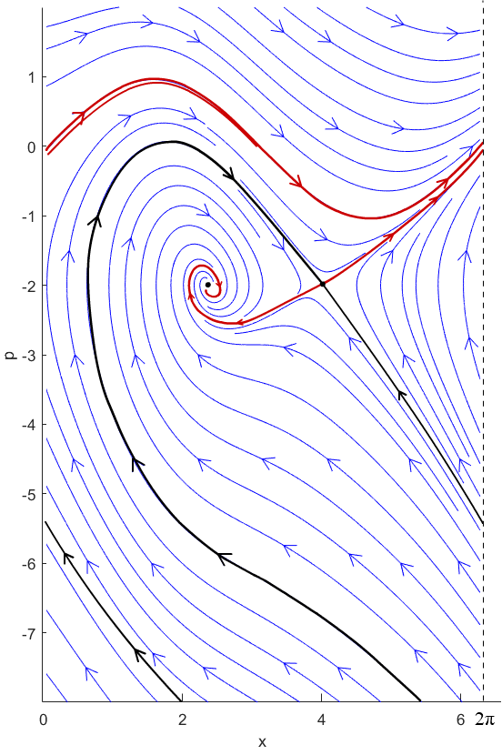
We should point out that usually $\mathcal{T}_{\omega}$ is not a global attractor and extra invariant sets may exist in the phase space (see Fig. 1). Nonetheless, the KAM torus is the only destination of all the variational minimal orbits as $t\rightarrow+\infty$ , not the extra invariant sets.

1.4. Is the Lagrangian graph variational stable?

Open Problem 1.

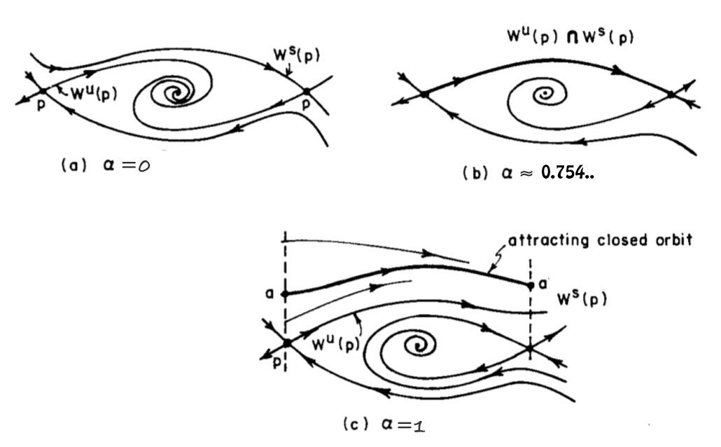
Does an invariant Lagrangian graph of a conformally symplectic system still persists as an invariant Lagrangian graph under small perturbation?

The answer to this question seems negative, as is shown in Fig. 2, the dissipative property of (2) leads to a bifurcation of the global attractor. For $\alpha$ equal to the bifurcate value $0.754...$ , the Lagrangian graph is a union of homoclinic orbit and a hyperbolic equilibrium (only Lipschitz smooth). If we reduce the value of $\alpha$ , the Lagrangian graph disappears and a non-graphic global attractor comes out, as shown in (a) of Fig. 2.

Since the KAM torus is normally hyperbolic, under small perturbation it persists as a $\Phi_{H,\lambda}^{t}-$ invariant $C^{1}-$ graph due to the Invariant Manifold Theorem [12], although the dynamic on the perturbed torus may no longer conjugate to a rotation. That implies the persistence of Lagrangian graphs is possible with prior KAM assumption:

Refer to caption — Figure 1. Example with a coexistence of KAM torus and fixed points: $H(x,p)=\frac{1}{2}(p+2)^{2}-2\sin x+\frac{1}{\sqrt{2}}\cos x+\frac{1}{4}\cos 2x$ , $\lambda=\frac{1}{\sqrt{2}}$ . The KAM torus equals $\{(x,\sin x)|x\in\mathbb{T}\}$ . The maximal global attractor defined in [15] is marked in red.

Theorem 5.

(proved in Sec. 5) The KAM torus of a conformally symplectic system keeps to be a $C^{1}-$ Lagrangian graph under small perturbations.

Organization of the article: The paper is organized as follows: In Sec. 2, we give a brief introduction about the the weak KAM theory. In Sec. 3, we prove the symplectic properties of the KAM torus, i.e. Theorem 1 and Theorem 2. In Sec. 4, we discuss the $C^{1}-$ convergence of the Lax-Oleinik semigroup and prove Theorem 4. In Sec. 5 we prove the Lagrangian persistence of the KAM toruus, namely Theorem 5. For the consistency of the proof, some longsome and independent conclusions are moved to the Appendix.

Acknowledgements: Jianlu Zhang is supported by the National Natural Science Foundation of China (Grant No. 11901560). The authors are grateful to Prof. A Sorrentino for checking the proof of exactness of the Lagrangian graphs and giving constructive suggestions.

2. Weak KAM theory of discounted H-J equations

In this section we display a list of definitions and conclusions about the variational principle of system (2), which can be used in later sections.

Definition 2.1 (Viscosity solution).

(1)

A function $u:\mathbb{T}^{n}\to\mathbb{R}$ is called a viscosity subsolution (resp. viscosity supersolution) of equation (7), if for every $C^{1}$ function $\varphi:\mathbb{T}^{n}\rightarrow\mathbb{R}$ and every point $x_{0}\in\mathbb{T}^{n}$ at which $u-\varphi$ reaches a local maximum (resp. minimum) , we have

$H(x_{0},\partial_{x}\varphi(x_{0}))+\lambda u(x_{0})\leqslant 0\quad(resp.\geqslant 0);$
(2)

A function $u:\mathbb{T}^{n}\to\mathbb{R}$ is called a viscosity solution of equation (7), if it is both a viscosity subsolution and a viscosity supersolution.
(3)

Similarly, a function $U:\mathbb{T}^{n}\times[0,+\infty)\rightarrow\mathbb{R}$ can be defined by the viscosity subsolution, viscosity supersolution or viscosity solution of equation (6), if aforementioned items holds in the interior region $(0,+\infty)\times M$ for $U$ respectively.

Proposition 2.2.

(1)

(Variational principle) For each $\psi\in C(\mathbb{T}^{n},\mathbb{R})$ , each $x\in\mathbb{T}^{n}$ and each $t\geqslant 0$ , we can find a $C^{2}$ smooth curve $\gamma_{x,t}:\tau\in[-t,0]\rightarrow\mathbb{T}^{n}$ ending with $x$ such that

\displaystyle\mathcal{T}^{-}_{t}\psi(x)=\,e^{-\lambda t}\psi(\gamma_{x,t}(-t))+\int_{-t}^{0}e^{\lambda\tau}L(\gamma_{x,t}(\tau),\dot{\gamma}_{x,t}(\tau))d\tau.

Moreover, $\mathcal{L}_{H}^{-1}(\gamma_{x,t}(\tau),\dot{\gamma}_{x,t}(\tau))$ satisfies (2) for $\tau\in(-t,0)$ .

(2)

(Pre-compactness) for any $\psi\in C(\mathbb{T}^{n},\mathbb{R})$ and any $t\geqslant 1$ , there exists a constant $K:=K(L,\lambda)>0$ depending only on $L$ and $\lambda$ , such that the minimizing curve $\gamma_{x,t}$ achieving $\mathcal{T}_{t}^{-}\psi$ satisfies $|\dot{\gamma}_{x,t}(\tau)|\leqslant K$ for all $\tau\in(-t,0)$ .
(3)

(Viscosity solution) Suppose $U_{\psi}(x,t):=\mathcal{T}_{t}^{-}\psi(x)$ , then it is a viscosity solution of the EdH-J equation (6).

Proof.

For assertion (1), by taking

(9)

\displaystyle h_{\lambda}^{t}(y,x):=\inf_{\begin{subarray}{c}\gamma\in C^{ac}([-t,0],\mathbb{T}^{n})\\ \gamma(-t)=y\ \gamma(0)=x\end{subarray}}\int_{-t}^{0}e^{\lambda\tau}L(\gamma,\dot{\gamma})\ d\tau,

we get a simplified expression

\mathcal{T}_{t}^{-}\psi(x)=\inf_{y\in\mathbb{T}^{n}}\{e^{-\lambda t}\psi(y)+h_{\lambda}^{t}(y,x)\}.

Since the function $y\mapsto e^{-\lambda t}\psi(y)+h_{\lambda}^{t}(y,x)$ is continuous on $\mathbb{T}^{n}$ , we can find $y_{x,t}\in\mathbb{T}^{n}$ such that $\mathcal{T}_{t}^{-}\psi(x)=e^{-\lambda t}\psi(y_{x,t})+h_{\lambda}^{t}(y_{x,t},x)$ . Due to the Tonelli Theorem, the infimum of $h^{t}_{\lambda}(y,x)$ in (9) is always achievable, and has to be $C^{2}-$ smooth due to the Weierstrass Theorem [17]. Hence, we can find a $C^{2}$ smooth curve $\gamma_{x,t}:[-t,0]\to\mathbb{T}^{n}$ with $\gamma_{x,t}(-t)=y_{x,t}$ and $\gamma_{x,t}(0)=x$ such that

h_{\lambda}^{t}(y_{x,t},x)=\int_{-t}^{0}e^{\lambda\tau}L(\gamma_{x,t}(\tau),\dot{\gamma}_{x,t}(\tau))\ d\tau.

For assertion (2), as we know, for any $\psi\in C^{0}(\mathbb{T}^{n},\mathbb{R})$ and $t\geqslant 1$ ,we choose $0<\sigma<t$ such that $\frac{1}{2}\leqslant\sigma\leqslant 1$ , due to item (1), there exists a a $C^{2}$ smooth curve $\gamma_{x,t}:[-t,0]\mapsto\mathbb{T}^{n}$ with $\gamma_{x,t}(0)=x$ and due to $\mathcal{T}^{-}_{t}$ is a semigroup operator,

	$\displaystyle\mathcal{T}^{-}_{t}\psi(x)=$	$\displaystyle\,\inf_{y\in\mathbb{T}^{n}}\{e^{-\lambda t}\psi(y)+h_{\lambda}^{t}(y,x)\}$
	$\displaystyle=$	$\displaystyle\,\inf_{z\in\mathbb{T}^{n}}\{e^{-\lambda\sigma}\big{(}\mathcal{T}^{-}_{t-\sigma}\psi(z)\big{)}+h_{\lambda}^{\sigma}(z,x)\}$
	$\displaystyle=$	$\displaystyle\,e^{-\lambda\sigma}\mathcal{T}^{-}_{t-\sigma}\psi(\gamma_{x,t}(-\sigma))+h_{\lambda}^{\sigma}(\gamma_{x,t}(-\sigma),\gamma_{x,t}(0))$
	$\displaystyle=$	$\displaystyle\,e^{-\lambda\sigma}\mathcal{T}^{-}_{t-\sigma}\psi(\gamma_{x,t}(-\sigma))+\int_{-\sigma}^{0}e^{\lambda\tau}L(\gamma_{x,t}(\tau),\dot{\gamma}_{x,t}(\tau))d\tau$

By chosen $\eta:[-\sigma,0]\to\mathbb{R}$ being the straight line connecting $\gamma_{x,t}(-\sigma)$ and $\gamma_{x,t}(0)$ , we have

	$\displaystyle h_{\lambda}^{\sigma}(\gamma_{x,t}(\sigma),\gamma_{x,t}(0))\leqslant$	$\displaystyle\,\int_{-\sigma}^{0}e^{\lambda\tau}L(\eta(\tau),\dot{\eta}(\tau))d\tau$
	$\displaystyle\leqslant$	$\displaystyle\,C\int_{-\sigma}^{0}e^{\lambda\tau}d\tau$

for a suitable constant $C$ depending only on $L(x,v)$ with $|v|\leqslant diam(\mathbb{T}^{n})$ . On the other hand, there exists constants $k,l>0$ such that $L(x,v)\geqslant k|v|-l$ for all $(x,v)\in T\mathbb{T}^{n}$ , then

	$\displaystyle h_{\lambda}^{\sigma}(\gamma_{x,t}(-\sigma),\gamma_{x,t}(0))\geqslant$	$\displaystyle\,\int_{-\sigma}^{0}e^{\lambda\tau}(k\|\dot{\gamma}_{x,t}\|-l)d\tau$
	$\displaystyle\geqslant$	$\displaystyle\,k\int_{-\sigma}^{0}e^{\lambda\tau}\|\dot{\gamma}_{x,t}\|d\tau-l\int_{-\sigma}^{0}e^{\lambda\tau}d\tau.$

Hence, we have

\int_{-\sigma}^{0}|\dot{\gamma}_{x,t}|d\tau\leqslant\frac{l+C}{ke^{-\lambda\sigma}}\int_{-\sigma}^{0}e^{\lambda\tau}d\tau=\frac{l+C}{k\lambda}(e^{\lambda\sigma}-1).

There always exists a $t^{\prime}\in[-\sigma,0]$ such that $|\dot{\gamma}_{x,t}(t^{\prime})|\leqslant\frac{l+C}{k\lambda}\frac{e^{\lambda\sigma}-1}{\sigma}$ . Since $\gamma_{x,t}$ satisfies the (E-L), then $|\dot{\gamma}_{x,t}(\tau)|$ is uniformly bounded on $\tau\in[-\sigma,0]$ .

Choose $-t\leqslant-\sigma_{N}\leqslant-\sigma_{N-1}\leqslant\cdots\leqslant-\sigma_{1}\leqslant-\sigma_{0}=-\sigma\leqslant 0$ such that $\frac{1}{2}\leqslant\sigma_{i}-\sigma_{i+1}\leqslant 1$ , then for any $1\leqslant i\leqslant N$ we get

\mathcal{T}^{-}_{t-\sigma_{i-1}}\psi(\gamma_{x,t}(-\sigma_{i-1}))=e^{\lambda(\sigma_{i-1}-\sigma_{i})}\mathcal{T}^{-}_{t-\sigma_{i}}\psi(-\gamma_{x,t}(-\sigma_{i}))+\int_{-\sigma_{i}}^{-\sigma_{i-1}}e^{\lambda\tau}L(\gamma_{x,t}(\tau),\dot{\gamma}_{x,t}(\tau))d\tau,

the same scheme as above still works. So $|\dot{\gamma}_{x,t}(\tau)|$ is uniformly bounded on $\tau\in[-t,0]$ .

For assertion (3), it’s a classical conclusion in the Optimal Control Theory (e.g. [1, Chapter III]) that $U_{\psi}(x,t):=\mathcal{T}_{t}^{-}\psi(x)$ is a continuous viscosity solution of (7). Here we give a sketch:

To prove $U_{\psi}(x,t)=\mathcal{T}_{t}^{-}\psi(x)$ is a subsolution; for any fixed $(x_{0},t_{0})\in\mathbb{T}^{n}\times(0,+\infty)$ . Let $\varphi$ be a $C^{1}$ test function such that $(x_{0},t_{0})$ is a local maximal point of $U_{\psi}-\varphi$ and $U_{\psi}(x_{0},t_{0})=\varphi(x_{0},t_{0})$ . That is

(10)

\displaystyle\varphi(x_{0},t_{0})-\varphi(x,t)\leqslant U_{\psi}(x_{0},t_{0})-U_{\psi}(x,t),\quad(x,t)\in W,

with $W$ be an open neighborhood of $(x_{0},t_{0})$ in $\mathbb{T}^{n}\times(0,+\infty)$ .

Due to item(1) and $\mathcal{T}_{t}^{-}$ is a semigroup operator, for any differentiable point $x_{2}\in W$ , we have that $\mathcal{T}_{t_{2}-t_{1}}^{-}\circ\mathcal{T}_{t_{1}}^{-}\psi(x_{2})=\mathcal{T}_{t_{2}}^{-}\psi(x_{2})$ for any $t_{1}<t_{2}$ in $W$ which implies that

\displaystyle e^{\lambda t_{2}}U_{\psi}(x_{2},t_{2})-e^{\lambda t_{1}}U_{\psi}(x_{1},t_{1})\leqslant\,\int^{t_{2}}_{t_{1}}e^{\lambda\tau}L(\gamma,\dot{\gamma})d\tau.

for any $C^{1}$ curve $\gamma:[t_{1},t_{2}]\to\mathbb{T}^{n}$ connecting $x_{1}$ to $x_{2}$ . By (10) it follows

\displaystyle\varphi(t_{2},x_{2})-\varphi(t_{1},x_{1})\leqslant\int^{t_{2}}_{t_{1}}e^{\lambda(\tau-t_{2})}L(\gamma,\dot{\gamma})d\tau-(1-e^{\lambda(t_{1}-t_{2})})U_{\psi}(x_{1},t_{1}).

By letting $|t_{2}-t_{1}|\to 0$ , this gives rise to

\displaystyle\partial_{t}\varphi(x_{0},t_{0})+\partial_{x}\varphi(x_{0},t_{0})\cdot\dot{\gamma}(t_{0})\leqslant L(x_{0},\dot{\gamma}(t_{0}))-\lambda U_{\psi}(x_{0},t_{0})

As an application of Fenchel-Legendre dual, we obtain

\displaystyle\partial_{t}\varphi(x_{0},t_{0})+H(x_{0},\partial_{x}\varphi(x_{0},t_{0}))+\lambda U_{\psi}(x_{0},t_{0})\leqslant 0,

which shows that $U_{\psi}$ is a subsolution.

Now we turn to the proof that $U_{\psi}$ is a supersolution. Let $\varphi$ be a $C^{1}$ test function such that $(x_{0},t_{0})$ is a local minimal point of $u-\varphi$ and $U_{\psi}(x_{0},t_{0})=\varphi(x_{0},t_{0})$ . That is

\displaystyle\varphi(x_{0},t_{0})-\varphi(x,t)\geqslant U_{\psi}(x_{0},t_{0})-U_{\psi}(x,t),\quad(x,t)\in V,

with $V$ be an open neighborhood of $(x_{0},t_{0})$ in $\mathbb{T}^{n}$ . There exists a $C^{2}$ curve $\xi:[t,t_{0}]\to V$ with $\xi(t_{0})=x_{0}$ such that

\displaystyle U_{\psi}(\xi(t_{0}),t_{0})-U_{\psi}(\xi(t),t)=\int^{t_{0}}_{t}L(\xi,\dot{\xi})-\lambda U_{\psi}(\xi(s),s)\ ds.

Hence

\displaystyle\varphi(x_{0},t_{0})-\varphi(\xi(t),t)\geqslant\int^{t_{0}}_{t}L(\xi,\dot{\xi})-\lambda U_{\psi}(\xi(s),s)\ ds,

It follows that

\displaystyle\partial_{t}\varphi(x_{0},t_{0})+\partial_{x}\varphi(x_{0},t_{0})\cdot\dot{\xi}(t_{0})\geqslant L(x_{0},\dot{\xi}(t_{0}))-\lambda U_{\psi}(x_{0},t_{0}),

which implies

\displaystyle\partial_{t}\varphi(x_{0},t_{0})+H(x_{0},\partial_{x}\varphi(t_{0},x_{0}))+\lambda U_{\psi}(x_{0},t_{0})\geqslant 0.

So we finally finish the proof. ∎

Proposition 2.3.

(1)

(Expression) [6, Theorem 6.1] For all $\psi\in C^{0}(M,\mathbb{R})$ , the limit of $\mathcal{T}_{t}^{-}\psi(x)$ exists and can be explicitly expressed, i.e.

(11)

\displaystyle\lim_{t\rightarrow+\infty}\mathcal{T}_{t}^{-}\psi=\inf_{\begin{subarray}{c}\gamma\in C^{ac}((-\infty,0],\mathbb{T}^{n})\\ \gamma(0)=x\end{subarray}}\int_{-\infty}^{0}e^{\lambda\tau}L(\gamma,\dot{\gamma})d\tau.

Since the limit is independent of $\psi$ , we can denote it by $u^{-}(x)$ .

(2)

(Domination) [6, Proposition 6.3] For any absolutely continuous curve $\gamma:[a,b]\rightarrow\mathbb{T}^{n}$ connecting $x,y\in\mathbb{T}^{n}$ , we have

(12)

\displaystyle e^{\lambda b}u^{-}(y)-e^{\lambda a}u^{-}(x)\leqslant\int_{a}^{b}e^{\lambda\tau}L(\gamma,\dot{\gamma})d\tau.

(3)

(Calibration)[6, Proposition 6.2] For any $x\in\mathbb{T}^{n}$ , there exists a $C^{r}$ backward calibrated curve $\gamma_{x}^{-}:(-\infty,0]\rightarrow\mathbb{T}^{n}$ ending with $x$ , such that for all $s\leqslant t\leqslant 0$ , we have

(13)

\displaystyle e^{\lambda t}u^{-}(\gamma_{x}^{-}(t))-e^{\lambda s}u^{-}(\gamma_{x}^{-}(s))=\int_{s}^{t}e^{\lambda\tau}L(\gamma_{x}^{-},\dot{\gamma}_{x}^{-})d\tau.

Similarly, $\mathcal{L}_{H}^{-1}(\gamma_{x}^{-}(\tau),\dot{\gamma}_{x}^{-}(\tau))$ satisfies (2) for $\tau\in(-\infty,0)$ .

(4)

(Pre-compactness)[6, Proposition 6.2] There exists a constant $K>0$ depending only on $L$ , such that the minimizing curve $\gamma_{x}^{-}$ of $u^{-}(x)$ satisfies $|\dot{\gamma}_{x}^{-}(\tau)|\leqslant K$ , for all $\tau\in(-\infty,0)$ .
(5)

[15, Proposition 5,6] Along each calibrated curve $\gamma_{x}^{-}:(-\infty,0]\rightarrow\mathbb{T}^{n}$ , we have

$\lambda u^{-}(\gamma_{x}^{-}(s))+H(\gamma_{x}^{-}(s),d_{x}u^{-}(\gamma_{x}^{-}(s)))=0,\quad\forall s<0.$
(6)

( $C^{0}-$ convergent speed) Let $U_{\psi}(x,t):=\mathcal{T}_{t}^{-}\psi$ be the viscosity solutions of the equation (6), there exists a constant $C_{1}=C_{1}(\psi,L,\lambda)$ , such that

$\big{\|}U_{\psi}(x,t)-u^{-}(x)\big{\|}\leqslant C_{1}e^{-\lambda t},\quad\forall t\geqslant 1.$
(7)

(Stationary solution) $u^{-}(x)$ is a viscosity solution of (7).

Proof.

As direct citations, we have marked the exact references for the first five items of this Proposition. For item (6), due to the expression of $u^{-}(x)$ in (11) and item (3), there must exist an absolutely continuous curve $\gamma_{x}^{-}:(-\infty,0]\rightarrow\mathbb{T}^{n}$ with $\gamma_{x}^{-}(0)=x$ such that $u^{-}(x)=\int_{-\infty}^{0}e^{\lambda\tau}L(\gamma_{x}^{-},\dot{\gamma}_{x}^{-})d\tau.$ Then we have

		$\displaystyle\,U_{\psi}(x,t)-u^{-}(x)$
	$\displaystyle\leqslant$	$\displaystyle\,e^{-\lambda t}\psi(\gamma_{x}^{-}(-t))+\int_{-t}^{0}e^{\lambda\tau}L(\gamma_{x}^{-},\dot{\gamma}_{x}^{-})d\tau-\int_{-\infty}^{0}e^{\lambda\tau}L(\gamma_{x}^{-},\dot{\gamma}_{x}^{-})d\tau$
	$\displaystyle=$	$\displaystyle\,e^{-\lambda t}\psi(\gamma_{x}^{-}(-t))-\int_{-\infty}^{-t}e^{\lambda\tau}L(\gamma_{x}^{-},\dot{\gamma}_{x}^{-})d\tau$
	$\displaystyle\leqslant$	$\displaystyle\,e^{-\lambda t}\psi(\gamma_{x}^{-}(s))-\min_{(x,v)\in T\mathbb{T}^{n}}L(x,v)\int_{-\infty}^{-t}e^{\lambda\tau}d\tau$
	$\displaystyle\leqslant$	$\displaystyle\,e^{-\lambda t}\Big{[}\|\|\psi\|\|_{C^{0}}+\frac{1}{\lambda}\min_{(x,v)\in T\mathbb{T}^{n}}L(x,v)\big{]}$
	$\displaystyle=$	$\displaystyle\,\widetilde{C}_{1}e^{-\lambda t},$

where $\widetilde{C}_{1}$ is a constant depending on $||\psi||_{C^{0}},\lambda$ and $\min_{T\mathbb{T}^{n}}L(x,v)$ . On the other hand, there is an absolutely continuous curve $\gamma_{x,t}:[-t,0]\rightarrow\mathbb{T}^{n}$ with $\gamma^{-}_{x}(0)=x$ such that $U_{\psi}(x,t)$ attains the infimum in the formula (5), define $\xi:(-\infty,0]\rightarrow\mathbb{T}^{n}$ by $\xi(\tau)=\gamma_{x,t}(\tau)$ for $\tau\in[-t,0]$ and $\xi(\tau)\equiv\gamma_{x,t}(-t)$ for $\tau\leqslant-t$ , it follows that $\xi$ is an absolutely continuous curve with $\xi(0)=x$ and

		$\displaystyle\,u^{-}(x)-U_{\psi}(x,t)$
	$\displaystyle\leqslant$	$\displaystyle\,\int_{-\infty}^{0}e^{\lambda\tau}L(\xi,\dot{\xi})d\tau-e^{-\lambda t}\psi(\xi(-t))-\int_{-t}^{0}e^{\lambda\tau}L(\xi,\dot{\xi})d\tau$
	$\displaystyle\leqslant$	$\displaystyle\,e^{-\lambda t}\|\psi(\xi(-t))\|+\int_{-\infty}^{-t}e^{\lambda\tau}L(\xi,\dot{\xi})d\tau$
	$\displaystyle\leqslant$	$\displaystyle\,e^{-\lambda t}\big{[}\|\|\psi\|\|_{C^{0}}+\frac{1}{\lambda}\max_{x\in\mathbb{T}^{n}}\|L(x,0)\|\big{]}$
	$\displaystyle=$	$\displaystyle\,\widetilde{C}_{2}e^{-\lambda t},$

with $\widetilde{C}_{2}$ being a constant depending on $||\psi||_{C^{0}},\lambda$ and $\max_{x\in\mathbb{T}^{n}}|L(x,0)|$ . Combining previous two inequalities we prove this item.

For item (7), the proof is similar with item (4) of Proposition 2.2. ∎

3. Exactness of the KAM torus

Proof of Theorem 1: The invariance of $\Sigma$ implies for any $x\in\mathbb{T}^{n}$ ,

\Phi^{t}_{H,\lambda}\Big{(}x,P(x)\Big{)}=\Big{(}x(t),P\big{(}x(t)\big{)}\Big{)},\quad\forall t\in\mathbb{R}.

Due to (2), for any $x\in\mathbb{T}^{n}$ ,

(14)	$\displaystyle-H_{x}(x,P(x))-\lambda P(x)$	$\displaystyle=$	$\displaystyle\dot{p}(0)$
		$\displaystyle=$	$\displaystyle\,\frac{dP\big{(}x(t)\big{)}}{dt}\bigg{\|}_{t=0}=d_{x}P(x)\cdot\dot{x}(0)$
		$\displaystyle=$	$\displaystyle\langle d_{x}P(x),H_{p}(x,P(x))\rangle.$

On the other side, we define

G(x):=\lambda u(x)+H(x,P(x))\in C^{1}(\mathbb{T}^{n},\mathbb{R}),

which satisfies

(15)	$\displaystyle d_{x}G(x)$	$\displaystyle=$	$\displaystyle\lambda d_{x}u(x)+d_{x}H(x,P(x))$
		$\displaystyle=$	$\displaystyle\,\langle d_{x}P(x),H_{p}(x,P(x))\rangle dx+\lambda d_{x}u(x)dx+H_{x}(x,P(x))dx$
		$\displaystyle=$	$\displaystyle\,\lambda[d_{x}u(x)-P(x)]dx=\,-\lambda cdx$

since $P(x)=c+d_{x}u(x)$ . We can read through previous equality for $i=1,...,n$ ,

\partial_{x_{i}}G(x)+\lambda c_{i}=0.

By integrating the above equality w.r.t. $x_{i}$ over $\mathbb{T}$ , then $c_{i}=0$ for $i=1,...,n$ .∎

Proof of Theorem 2: It suffices to show that $\Omega(T\mathcal{T}_{\omega},T\mathcal{T}_{\omega})=0$ , which is equivalent to show $K^{*}\Omega\big{|}_{T\mathbb{T}^{n}}=0$ . Recall that

\displaystyle(\Phi_{H,\lambda}^{t}\circ K)^{*}\Omega=K^{*}(\Phi_{H,\lambda}^{t})^{*}\Omega=e^{\lambda t}K^{*}\Omega.

On the other side, $K\circ\rho_{\omega}^{t}=\Phi_{H,\lambda}^{t}\circ K$ , which implies

(K\circ\rho_{\omega}^{t})^{*}\Omega=(\rho_{\omega}^{t})^{*}K^{*}\Omega.

Combining these two equalities we get

(\rho_{\omega}^{-t})^{*}K^{*}\Omega=e^{-\lambda t}K^{*}\Omega,\quad\forall\ t\in\mathbb{R}_{+}.

Since $\mathcal{T}_{\omega}$ is $\Phi_{H,\lambda}^{t}-$ invariant, and $\lim_{t\rightarrow+\infty}(\rho_{\omega}^{-t})^{*}K^{*}\Omega=0$ , we prove $K^{*}\Omega=0$ .∎

4. $W^{1,\infty}-$ convergence speed of the Lax-Oleinik semigroup

4.1. Semiconcave functions with linear modulus

Definition 4.1 (Hausdorff metric).

Let $(X,d)$ be a metric space and $\mathcal{K}(X)$ be the set of non-empty compact subset of $X$ . The Hausdorff metric $d_{H}$ induced by $d$ is defined by

d_{H}(K_{1},K_{2})=\max\big{\{}\max_{x\in K_{1}}d(x,K_{2}),\max_{x\in K_{2}}d(K_{1},x)\big{\}},\quad\forall K_{1},K_{2}\in\mathcal{K}(X)

Definition 4.2 (SCL).

Let $\mathcal{U}\subset\mathbb{R}^{n}$ be a open set. A function $f:\mathcal{U}\to\mathbb{R}$ is said to be semiconcave with linear modulus (SCL for short) if there exists a constant $C>0$ such that

\lambda f(x)+(1-\lambda)f(y)-f(\lambda x+(1-\lambda)y)\leqslant\frac{C}{2}\lambda(1-\lambda)|x-y|^{2}\quad\forall x,y\in\mathcal{U},\ \forall\lambda\in[0,1].

Definition 4.3.

Assume $f\in C(\mathcal{U},\mathbb{R})$ , for any $x\in\mathcal{U}$ , the closed convex set

D^{+}f(x)=\Big{\{}\eta\in T^{*}\mathcal{U}:\limsup_{|h|\to 0}\frac{f(x+h)-f(x)-\langle\eta,h\rangle}{|h|}\leqslant 0\Big{\}}

\Big{(}\ \text{resp.}\ D^{-}f(x)=\Big{\{}\eta\in T^{*}\mathcal{U}:\limsup_{|h|\to 0}\frac{f(x+h)-f(x)-\langle\eta,h\rangle}{|h|}\geqslant 0\Big{\}}\Big{)}

is called the super-differential (resp. sub-differential) set of $f$ at $x$ .

Definition 4.4.

Suppose $f:\mathcal{U}\to\mathbb{R}$ is local Lipschitz. A vector $p\in T^{*}\mathcal{U}$ is called a reachable gradient of $u$ at $x\in\mathcal{U}$ if a sequence $\{x_{k}\}_{k\in\mathbb{N}}\subset\mathcal{U}\backslash\{x\}$ exists such that $f$ is differentiable at $x_{k}$ for each $k\in\mathbb{N}$ , and

\lim_{k\to\infty}x_{k}=x,\quad\lim_{k\to\infty}d_{x}f(x_{k})=p.

The set of all reachable gradients of $f$ at $x$ is denoted by $D^{*}f(x)$ .

Lemma 4.5.

[4, Theorem.3.1.5(2)] $f:\mathcal{U}\subset\mathbb{R}^{d}\rightarrow\mathbb{R}$ is a SCL, then $D^{+}f(x)$ is a nonempty compact convex set for any $x\in\mathcal{U}$ .

Theorem 6.

[4, Theorem.3.3.6] Let $f:\mathcal{U}\to\mathbb{R}$ be a semiconcave function. For any $z\in\mathcal{U}$ ,

D^{+}f(z)=coD^{*}f(z),

i.e. any element in $D^{+}f(z)$ can be expressed as a convex combination of elements in $D^{*}f(z)$ . As a corollary, ex $(D^{+}f(z))\subset D^{*}f(z)$ , i.e. any extremal element of $D^{+}f(z)$ has to be contained in $D^{*}f(z)$ .

Theorem 7.

[4, Th. 5.3.8] For any fixed $t>0$ , the viscosity solutions $U_{\psi}(x,t):=\mathcal{T}_{t}^{-}\psi(x)$ (resp. $u^{-}(x)$ ) of (6) (resp. (7)) is $SCL_{loc}$ (resp. SCL) on $\mathbb{T}^{n}\times(0,+\infty)$ (resp. $\mathbb{T}^{n}$ ).

Theorem 8.

For any $x\in\mathbb{T}^{n}$ (resp. $(x,t)\in\mathbb{T}^{n}\times(0,+\infty)$ ) and $p\in D^{*}u^{-}(x)$ (resp. $(p_{t},p_{x})\in D^{*}U_{\psi}(x,t)$ ),there is a minimal curve $\gamma_{x}^{-}:(-\infty,0]\rightarrow\mathbb{T}^{n}$ (resp. $\gamma_{x,t}:[-t,0]\rightarrow\mathbb{T}^{n}$ ) satisfying

u^{-}(x)=\int_{-\infty}^{0}e^{\lambda\tau}L(\gamma_{x}^{-}(\tau),\dot{\gamma}_{x}^{-}(\tau))d\tau.

\displaystyle\bigg{(}resp.\quad U_{\psi}(x,t)=e^{-\lambda t}\psi(\gamma_{x,t}(-t))+\int_{-t}^{0}e^{\lambda\tau}L(\gamma_{x,t}(\tau),\dot{\gamma}_{x,t}(\tau))d\tau\bigg{)}

and

\lim_{s\rightarrow 0_{-}}\dot{\gamma}_{x}^{-}(s)=\frac{\partial H}{\partial p}(x,p)\quad\bigg{(}resp.\quad\lim_{s\rightarrow 0_{-}}\dot{\gamma}_{x,t}(s)=\frac{\partial H}{\partial p}(x,p_{x})\bigg{)}.

Conversely, for any calibrated curve $\gamma_{x}^{-}:(-\infty,0]\rightarrow\mathbb{T}^{n}$ (resp. $\gamma_{x,t}:[-t,0]\rightarrow\mathbb{T}^{n}$ ) ending at $x$ , the left derivative at $s=0$ (resp. $s=0$ ) exists and satisfies

\lim_{s\rightarrow 0_{-}}L_{v}(\gamma_{x}^{-}(s),\dot{\gamma}_{x}^{-}(s))\in D^{*}u^{-}(x)

\bigg{(}resp.\quad\begin{pmatrix}\lim_{s\rightarrow 0_{-}}L_{v}(\gamma_{x,t}(s),\dot{\gamma}_{x,t}(s))\\ -\lim_{s\rightarrow 0_{-}}\lambda U_{\psi}(\gamma_{x,t}(s),s)+H(\gamma_{x,t}(s),L_{v}(\gamma_{x,t}(s),\dot{\gamma}_{x,t}(s)))\end{pmatrix}\in D^{*}U_{\psi}(x,t)\bigg{)}.

Proof.

If $u^{-}$ is differentiable at $x$ , by item (3) of Proposition 2.3, there exists a unique $\lambda-$ calibrated curve $\gamma_{x}^{-}:(-\infty,0]\rightarrow\mathbb{T}^{n}$ ending with $x$ , such that $u^{-}(\gamma_{x}^{-}(s))$ is differentiable for any $s\in(-\infty,0)$ , which implies

(16)

(x,\lim_{\tau\rightarrow 0_{-}}\dot{\gamma}^{-}_{x}(\tau))=\mathcal{L}_{H}^{-1}(x,d_{x}u^{-}(x)).

Equivalently, $(\xi(s),p(s)):=(\gamma^{-}_{x}(s),d_{x}u^{-}(\gamma_{x}^{-}(s)))$ solving

(17)

\displaystyle\begin{split}\begin{cases}\dot{\xi}(s)=\partial_{p}H(\xi(s),p(s)),\\ \dot{p}(s)=-\partial_{x}H(\xi(s),p(s))-\lambda p(s)\end{cases}\end{split}

for $s\in(-\infty,0]$ .

If $x\in\mathbb{T}^{n}$ is a non-differentiable point of $u^{-}$ , then for any $p_{x}\in D^{*}u^{-}(x)$ , there exists a sequence $\{x_{k}\}_{k\in\mathbb{N}}$ of differentiable points of $u^{-}$ converging to $x$ , such that $p=\lim_{k\to\infty}d_{x}u^{-}(x_{k})$ . Due to item (5) of Proposition 2.3 we have

\lambda u^{-}(x_{k})+H(x_{k},d_{x}u^{-}(x_{k}))=0

and there exists minimizing curves $\{\gamma_{x_{k}}^{-}\}_{k\in\mathbb{N}}$ solving (17), such that by letting $k\to\infty$ , we get

\lambda u^{-}(x)+H(x,p_{x})=0.

Due to the uniqueness of the solution of (17), the limit curve $\gamma_{x}^{-}:(-\infty,0]\rightarrow\mathbb{T}^{n}$ of the sequence of minimizing curves $\{\gamma_{x_{k}}^{-}\}_{k\in\mathbb{N}}$ has to be unique as well, with the terminal conditions $\gamma_{x}^{-}(0)=x,\ p(0)=p_{x}$ . This proves that the correspondence

\Upsilon:p_{x}\in D^{*}u^{-}(x)\to\gamma_{x}^{-}(\tau)\big{|}_{\tau\in(-\infty,0]}

is injective.

Now we prove the other direction. if $\gamma\in C^{ac}((-\infty,0],\mathbb{T}^{n})$ is $\lambda$ -calibrated by $u^{-}$ with $\gamma(0)=x$ , due to item (4) and (7) of Proposition 2.3 $u^{-}$ is differentiable at $\gamma(s)$ and $\gamma$ is actually $C^{2}$ for any $s\in(-\infty,0)$ . Therefore, by (16) , setting

\displaystyle p_{x}=\lim_{s\rightarrow 0_{-}}d_{x}u^{-}(\gamma(s))=\lim_{s\rightarrow 0_{-}}L_{v}(\gamma(s),\dot{\gamma}(s)),

there holds $p_{x}\in D^{\ast}u(x)$ . By a similar analysis the conclusion can be proved for $U_{\psi}(x,t)$ , or see [4, Th.6.4.9] for a direct citation. ∎

4.2. Proof of Theorem 4

Based on aformentioned preparations, we turn to the proof of Theorem 4. Recall that the KAM torus $\mathcal{T}_{\omega}$ is the graph of $du^{-}$ (due to Theorem 3), where $u^{-}(x)$ is the unique $C^{2}-$ classic solution of (7). On the other side, $U_{\psi}(x,t)$ is SCL_loc w.r.t. $(x,t)\in\mathbb{T}^{n}\times(0,+\infty)$ , then $D^{+}U_{\psi}(x,t)$ has to be a compact convex set. Now we assume $t\geqslant 1$ , then for any $(p_{x},p_{t})\in D^{*}U_{\psi}(x,t)$ , due to Proposition 8 there is a unique minimizer curve $\gamma_{x,t}$ with $\gamma_{x,t}(0)=x$ such that

\displaystyle\quad U_{\psi}(x,t)=e^{-\lambda t}\psi(\gamma_{x,t}(0))+\int_{-t}^{0}e^{\lambda\tau}L(\gamma_{x,t}(\tau),\dot{\gamma}_{x,t}(\tau))d\tau

with $p_{x}=\lim_{\tau\to 0_{-}}d_{x}U_{\psi}(\gamma_{x,t}(\tau),\tau)$ . Moreover, the following properties of $u^{-}$ and $U_{\psi}$ can be proved easily:

Lemma 4.6.

(1)

For any fixed $x\in\mathbb{T}^{n}$ , we have

\displaystyle d_{H}(d_{x}u^{-}(x),\Pi_{x}D^{+}U_{\psi}(x,t))=\,\max_{\begin{subarray}{c}p_{x}\in\Pi_{x}D^{*}U_{\psi}(x,t)\end{subarray}}|d_{x}u^{-}(x)-p_{x}|

where $\Pi_{x}:T^{*}_{(x,t)}(\mathbb{T}^{n}\times\mathbb{T})\to T_{x}^{*}\mathbb{T}^{n}$ is the standard projection.

(2)

There exists a constant $C_{2}(\psi,L,\lambda)$ depending only on $\psi$ and $L$ , such that

\displaystyle|d_{x}u^{-}(x)-p_{x}|\leqslant C_{2}(\psi,L,\lambda)\lim_{\tau\to 0_{-}}|\dot{\gamma}_{x}^{-}(\tau)-\dot{\gamma}_{x,t}(\tau)|

(3)

There exists a constant $A:=A(\psi,L,\lambda)$ such that

(18)

\displaystyle\left\{\begin{aligned} &\,\big{|}\dot{\gamma}_{x,t}(\tau)\big{|},\big{|}\ddot{\gamma}_{x,t}(\tau)\big{|}\leqslant A\\ &\,\big{|}\dot{\gamma}_{x}^{-}(\tau)\big{|},\big{|}\ddot{\gamma}_{x}^{-}(\tau)\big{|}\leqslant A\end{aligned}\right.\quad\quad\tau\in(-t,0),\quad x\in\mathbb{T}^{n}.

Proof.

(1) Due to Lemma 6, $D^{+}U_{\psi}(x,t)=coD^{*}U_{\psi}(x,t)$ then by Definition 8 , it obtain

		$\displaystyle\,d_{H}(d_{x}u^{-}(x),\Pi_{x}D^{+}U_{\psi}(x,t))=\max_{\begin{subarray}{c}p_{x}\in\Pi_{x}D^{+}U_{\psi}(x,t)\end{subarray}}\|d_{x}u^{-}(x)-p_{x}\|$
	$\displaystyle=$	$\displaystyle\,\max_{\begin{subarray}{c}p_{x}\in co\Pi_{x}D^{}U_{\psi}(x,t)\end{subarray}}\|d_{x}u^{-}(x)-p_{x}\|=\max_{\begin{subarray}{c}p_{x}\in\Pi_{x}D^{}U_{\psi}(x,t)\end{subarray}}\|d_{x}u^{-}(x)-p_{x}\|.$

(2) Since $\gamma_{x}^{-}(0)=\gamma_{x,t}(0)=x$ , due to Theorem 8 and item (5) of Proposition 2.3, we obtain that

	$\displaystyle p_{x}=\lim_{\tau\to 0_{-}}d_{x}U_{\psi}(\gamma_{x,t}(\tau),\tau)=\lim_{\tau\to 0_{-}}L_{v}(\gamma_{x,t}(\tau),\dot{\gamma}_{x,t}(\tau)),$
	$\displaystyle d_{x}u^{-}(x)=\lim_{\tau\to 0_{-}}d_{x}u^{-}(\gamma_{x}^{-}(\tau),\tau)=\lim_{\tau\to 0_{-}}L_{v}(\gamma_{x}^{-}(\tau),\dot{\gamma}_{x}^{-}(\tau)).$

Due to item(2) of Proposition 2.2 and item(4) of Proposition 2.3, we have

	$\displaystyle\|d_{x}u^{-}(x)-p_{x}\|\leqslant$	$\displaystyle\,\lim_{\tau\to 0_{-}}\|L_{v}(\gamma_{x}^{-}(\tau),\dot{\gamma}_{x}^{-}(\tau))-L_{v}(\gamma_{x,t}(\tau),\dot{\gamma}_{x,t}(\tau))\|$
	$\displaystyle\leqslant$	$\displaystyle\,C_{2}(\psi,L,\lambda)\lim_{\tau\to 0_{-}}\|\dot{\gamma}_{x}^{-}(\tau)-\dot{\gamma}_{x,t}(\tau)\|.$

(3) Denote that $p(\tau)=L_{v}(\gamma_{x,t}(\tau),\dot{\gamma}_{x,t}(\tau))$ , due to dissipative equation (2), we have

	$\displaystyle\,\ddot{\gamma}_{x,t}(\tau)=\frac{d}{dt}H_{p}\big{(}\gamma_{x,t}(\tau),p(\tau)\big{)}=H_{px}(\gamma_{x,t}(\tau),p(\tau))\cdot H_{p}(\gamma_{x,t}(\tau),p(\tau))$
	$\displaystyle\,\quad\quad\quad\quad\quad\quad\quad\quad\quad+H_{pp}(\gamma_{x,t}(\tau),p(\tau))(-H_{x}(\gamma_{x,t}(\tau),p(\tau))-\lambda p(\tau))\quad\tau\in(-t,0).$

By item(2) of Proposition 2.2 and item(4) of Proposition 2.3, for any $\tau\in(-t,0)$ , $(\gamma_{x,t}(\tau),\dot{\gamma}_{x,t}(\tau))$ and $(\gamma_{x}^{-}(\tau),\dot{\gamma}_{x}^{-}(\tau))$ fall in both a compact set of $\mathbb{T}^{n}$ . Hence, there exists a constant $A:=A(\psi,L,\lambda)$ such that $\big{|}\dot{\gamma}_{x,t}(\tau)\big{|},\big{|}\ddot{\gamma}_{x,t}(\tau)\big{|}\leqslant A$ and $\big{|}\dot{\gamma}_{x,t}(\tau)\big{|},\big{|}\ddot{\gamma}_{x,t}(\tau)\big{|}\leqslant A$ for any $\tau\in(-t,0)$ , even for $\tau\in[-t,0]$ if we consider the unilateral limit. This completes the proof. ∎

Now we define a substitute Lagrangian

(

\star

)

l(x,w):=L(x,w)-\lambda u^{-}(x)-\langle w,d_{x}u^{-}(x)\rangle

on $(x,w)\in T\mathbb{T}^{n}$ . Due to item (3) of Proposition 2.3, there exists a $\lambda-$ calibrated curve $\gamma_{x}^{-}:(-\infty,0]\rightarrow\mathbb{T}^{n}$ , of which

u^{-}(x)-e^{-\lambda t}u^{-}(\gamma_{x}^{-}(-t))=\int_{-t}^{0}e^{\lambda\tau}L(\gamma_{x}^{-},\dot{\gamma}_{x}^{-})d\tau

and

		$\displaystyle\,u^{-}(x)-e^{-\lambda t}u^{-}(\gamma_{x}^{-}(-t))=\int_{-t}^{0}\frac{d}{d\tau}\big{[}e^{\lambda\tau}u^{-}(\gamma_{x}^{-}(\tau))\big{]}\ d\tau$
	$\displaystyle=$	$\displaystyle\,\int_{-t}^{0}e^{\lambda\tau}\Big{[}\dot{\gamma}_{x}^{-}(\tau)\cdot d_{x}u^{-}+\lambda u^{-}\Big{]}\ d\tau.$

Therefore, we have

(19)

\displaystyle\int_{-t}^{0}e^{\lambda\tau}l(\gamma_{x}^{-}(\tau),\dot{\gamma}_{x}^{-}(\tau))\ d\tau=0

and

(20)

\displaystyle\int_{-t}^{0}e^{\lambda\tau}l(\eta(\tau),\dot{\eta}(\tau))\ d\tau\geqslant 0

for any $C^{1}-$ curve $\eta:[-t,0]\rightarrow\mathbb{T}^{n}$ , due to item (2) of Proposition 2.3.

Lemma 4.7.

Suppose $t\geqslant\sigma$ for some $\sigma>0$ , then there exists a constant $\alpha_{0}:=\alpha_{0}(\psi,L,\lambda)$ depending only on $L,\psi,\lambda$ such that

(21)

\displaystyle\left\{\begin{aligned} \int^{0}_{-\sigma}e^{\lambda\tau}l(\gamma_{x,t}(\tau),\dot{\gamma}_{x,t}(\tau))\ d\tau\leqslant&\,2C_{1}(\psi,L,\lambda)\ e^{-\lambda t},\\ \int^{0}_{-\sigma}e^{\lambda\tau}l(\gamma_{x,t}(\tau),\dot{\gamma}_{x,t}(\tau))\ d\tau\geqslant&\,\alpha_{0}(\psi,L,\lambda)\int^{0}_{-\sigma}e^{\lambda\tau}\big{|}\dot{\gamma}_{x,t}(\tau)-\dot{\eta}_{x,t}(\tau)\big{|}^{2}\ d\tau,\end{aligned}\right.

where

(22)

\displaystyle\eta_{x,t}(r):=x-\int^{0}_{r}\frac{\partial H}{\partial p}(\gamma_{x,t}(\tau),d_{x}u^{-}(\gamma_{x,t}(\tau)))\ d\tau

for any $r\in(-\sigma,0)$ .

Proof.

By the definition of the solution semigroup $\mathcal{T}_{t}^{-}\psi(x)=U_{\psi}(x,t)$ and item (2) of Proposition 2.2, there exists a $C^{2}$ curve $\gamma_{x,t}:[s,t]\mapsto\mathbb{T}^{n}$ such that

U_{\psi}(x,t)=e^{-\lambda\sigma}U_{\psi}(\gamma_{x,t}(-\sigma),-\sigma)+\int_{-\sigma}^{0}e^{\lambda\tau}L(\gamma_{x,t}(\tau),\dot{\gamma}_{x,t}(\tau))\ d\tau,

By integrating function $l$ along $\gamma_{x,t}$ with $\gamma_{x,t}(0)=x$ over the interval $[-\sigma,0]$ , we obtain

		$\displaystyle\,\int^{0}_{-\sigma}e^{\lambda\tau}l(\gamma_{x,t}(\tau),\dot{\gamma}_{x,t}(\tau))\ d\tau+u^{-}(x)-e^{-\lambda\sigma}u^{-}(\gamma_{x,t}(-\sigma))$
	$\displaystyle=$	$\displaystyle\,\int^{0}_{-\sigma}e^{\lambda\tau}L(\gamma_{x,t}(\tau),\dot{\gamma}_{x,t}(\tau))\ d\tau=U_{\psi}(x)-e^{-\lambda\sigma}U_{\psi}(\gamma_{x,t}(-\sigma),-\sigma)$

which implies that

(23)

\begin{split}&\,\int^{0}_{-\sigma}e^{\lambda\tau}l(\gamma_{x,t}(\tau),\dot{\gamma}_{x,t}(\tau))\ d\tau\\ \leqslant&\,e^{-\lambda\sigma}\Big{|}u^{-}(\gamma_{x,t}(-\sigma))-U_{\psi}(\gamma_{x,t}(-\sigma),-\sigma)\Big{|}+|u^{-}(x)-U_{\psi}(x,t)|,\\ \leqslant&\,e^{-\lambda\sigma}C_{1}(\psi,L,\lambda)e^{-\lambda(t-\sigma)}+C_{1}(\psi,L,\lambda)e^{-\lambda t}\\ =&\,2C_{1}(\psi,L,\lambda)e^{-\lambda t}\end{split}

where $C_{1}(\psi,L)$ is the same constant as in item (6) of Proposition 2.3. On the other hand, we denote

(

\star\star

)

F(x,w):=l(x,w)+H(x,d_{x}u^{-}(x))+\lambda u^{-}(x),\quad(x,w)\in T\mathbb{T}^{n}

which verifies to be nonnegative by the Fenchel Transform. Moreover,

	$\displaystyle\frac{\partial F}{\partial w}(x,w)=$	$\displaystyle\,\frac{\partial l}{\partial w}(x,w)=\frac{\partial L}{\partial w}(x,w)-d_{x}u^{-}(x)$
	$\displaystyle\frac{\partial^{2}F}{\partial w^{2}}(x,w)=$	$\displaystyle\,\frac{\partial^{2}l}{\partial w^{2}}(x,w)=\frac{\partial^{2}L}{\partial w^{2}}(x,w)$

then $F(x,w)=0$ if and only if $w=\frac{\partial H}{\partial p}(x,d_{x}u^{-}(x))$ . Due to (H1), there exists $\alpha_{0}(\psi,L,\lambda)$ such that

(24)

\displaystyle F(\gamma_{x,t}(\tau),\dot{\gamma}_{x,t}(\tau))\geqslant\alpha_{0}(\psi,L,\lambda)\Big{|}\dot{\gamma}_{x,t}(\tau)-\frac{\partial H}{\partial p}(\gamma_{x,t}(\tau),d_{x}u^{-}(\gamma_{x,t}(\tau)))\Big{|}^{2}.

Recall that $H(x,d_{x}u^{-}(x),t)+\lambda u^{-}(x)=0$ and we introduce

\eta_{x,t}(r):=x-\int^{0}_{r}\frac{\partial H}{\partial p}(\gamma_{x,t}(\tau),d_{x}u^{-}(\gamma_{x,t}(\tau)))\ d\tau

for any $-\sigma<r<0$ . Thus

(25)

\dot{\eta}_{x,t}(\tau)=\frac{\partial H}{\partial p}(\gamma_{x,t}(\tau),d_{x}u^{-}(\gamma_{x,t}(\tau))).

Now from (24), we get

	$\displaystyle l(\gamma_{x,t}(\tau),\dot{\gamma}_{x,t}(\tau))\geqslant$	$\displaystyle\,\alpha_{0}(\psi,L,\lambda)\Big{\|}\dot{\gamma}_{x,t}(\tau)-\frac{\partial H}{\partial p}(\gamma_{x,t}(\tau),d_{x}u^{-}(\gamma_{x,t}(\tau)))\Big{\|}^{2}$
	$\displaystyle=$	$\displaystyle\,\alpha_{0}(\psi,L,\lambda)\big{\|}\dot{\gamma}_{x,t}(\tau)-\dot{\eta}_{x,t}(\tau)\big{\|}^{2}$

which completes the proof. ∎

Recall that $\mathcal{T}_{\omega}$ is the unique attractor in its local neighborhood $\mathcal{U}$ (see Appendix A). There exists a constant $\Delta_{0}=\Delta_{0}(\lambda,L,\psi)>0$ such that

dist(\mathcal{T}_{\omega},\partial\mathcal{U})\geqslant\frac{3}{2}\Delta_{0}C_{2}(\psi,L,\lambda)

can be guaranteed by chosing suitable $\mathcal{U}$ . Consequently, the following Lemma holds:

Lemma 4.8.

There exists a suitable constant $s_{0}=s_{0}(\psi,L,\lambda)\geqslant 1$ such that

\lim_{\tau\to 0_{-}}|\dot{\gamma}_{x,t}(\tau)-\dot{\gamma}_{x}^{-}(\tau)|\leqslant\frac{3}{2}\Delta_{0},\quad\quad\forall\ t\in[s_{0},+\infty),\;x\in\mathbb{T}^{n}

Proof.

For any $s\geqslant 1$ , we assume that

(

\odot

)

\lim_{\tau\to 0_{-}}|\dot{\gamma}_{x,t}(\tau)-\dot{\gamma}_{x}^{-}(\tau)|>\Delta_{0}

for some $t\geqslant s$ and $x\in\mathbb{T}^{n}$ . Otherwise, the assertion of this Lemma holds. Due to (18), there exists a constant

A_{0}(\psi,L):=\max\bigg{\{}A,\max_{(x,v)\in\mathbb{T}^{n}\times B(0,A)}\frac{\partial H}{\partial p}(x,L_{v}(x,v))\bigg{\}}

such that for any $\tau\in[-t,0]$

\displaystyle|\dot{\eta}_{x,t}(\tau)|=

\displaystyle\,\Big{|}\frac{\partial H}{\partial p}(\gamma_{x,t}(\tau),d_{x}u^{-}(\gamma_{x,t}(\tau)))\Big{|}=\Big{|}\frac{\partial H}{\partial p}(\gamma_{x,t}(\tau),L_{v}(\gamma_{x,t}(\tau),\dot{\gamma}_{x,t}(\tau))\Big{|}\leqslant A_{0}

where $B(0,A)$ is a disk centering at $0$ and of a radius $A:=A(\psi,L,\lambda)$ which has been given in item (3) of Lemma 4.6. On the other side, there exists $\sigma\in[0,t]$ such that

|\dot{\gamma}_{x,t}(\tau)-\dot{\eta}_{x,t}(\tau)|>\Delta_{0},\quad\tau\in(-\sigma,0]

and $|\dot{\gamma}_{x,t}(-\sigma)-\dot{\eta}_{x,t}(-\sigma)|=\Delta_{0}$ as long as $s$ suitably large. This is because

	$\displaystyle 2C_{1}(\psi,L,\lambda)e^{-\lambda t}\geqslant$	$\displaystyle\,\int^{0}_{-\sigma}e^{\lambda\tau}l(\gamma_{x,t}(\tau),\dot{\gamma}_{x,t}(\tau))\ d\tau$
	$\displaystyle\geqslant$	$\displaystyle\,\alpha_{0}\int^{0}_{-\sigma}e^{\lambda\tau}\big{\|}\dot{\gamma}_{x,t}(\tau)-\dot{\eta}_{x,t}(\tau)\big{\|}^{2}\ d\tau$
	$\displaystyle\geqslant$	$\displaystyle\,\frac{\alpha_{0}}{\lambda}\min_{\tau\in[-\sigma,0]}\big{\|}\dot{\gamma}_{x,t}(\tau)-\dot{\eta}_{x,t}(\tau)\big{\|}^{2}(1-e^{-\lambda\sigma})$
	$\displaystyle\geqslant$	$\displaystyle\,\frac{\alpha_{0}}{\lambda}\Delta_{0}^{2}(1-e^{-\lambda\sigma}).$

due to (21). Therefore, if we make

s_{0}:=\max\bigg{\{}-\frac{1}{\lambda}\ln\frac{\alpha_{0}\Delta_{0}^{2}}{\lambda C_{1}(\psi,L,\lambda)},\;-\frac{1}{\lambda}\ln\frac{\alpha_{0}\Delta_{0}^{2}}{C_{1}(\psi,L,\lambda)}\big{(}1-e^{-\frac{\lambda\Delta_{0}}{4A_{0}}}\big{)},\;1\bigg{\}}

then $\sigma\leqslant\frac{\Delta_{0}}{4A_{0}}$ since $t\geqslant s\geqslant s_{0}$ . Due to (25),

	$\displaystyle\lim_{\tau\to 0_{-}}\|\dot{\gamma}_{x,t}(\tau)-\dot{\gamma}_{x}^{-}(\tau)\|=$	$\displaystyle\,\lim_{\tau\to 0_{-}}\|\dot{\gamma}_{x,t}(\tau)-\dot{\eta}_{x,t}^{-}(\tau)\|$
	$\displaystyle\leqslant$	$\displaystyle\,\max_{\tau\in(-\sigma,0)}\|\dot{\gamma}_{x,t}(\tau)-\dot{\eta}_{x,t}^{-}(\tau)\|$
	$\displaystyle\leqslant$	$\displaystyle\,\big{\|}\dot{\gamma}_{x,t}(-\sigma)-\dot{\eta}_{x,t}(-\sigma)\big{\|}+\sigma\cdot\max_{\tau\in(-\sigma,0)}\big{\|}\ddot{\gamma}_{x,t}(\tau)-\ddot{\eta}_{x,t}(\tau)\big{\|}$
	$\displaystyle\leqslant$	$\displaystyle\Delta_{0}+2A_{0}\sigma\leqslant\,\frac{3}{2}\Delta_{0}$

for any possible $t\geqslant s$ and $x\in\mathbb{T}^{n}$ such that ( $\odot$ ‣ 4.2) holds. So we complete the proof. ∎

Proof of Theorem 4: For any $x\in\mathbb{T}^{n}$ and $t\geqslant s_{0}(\psi,L,\lambda)$ with $s_{0}$ given in Lemma 4.8, there holds

			$\displaystyle\max_{x\in\mathbb{T}^{n}}d_{H}\bigg{(}\Pi_{x}D^{+}\mathcal{T}_{t}^{-}\psi(x),P(x)\bigg{)}$
		$\displaystyle=$	$\displaystyle\max_{x\in\mathbb{T}^{n}}d_{H}(\Pi_{x}D^{*}U_{\psi}(x,t),d_{x}u^{-})$
		$\displaystyle=$	$\displaystyle\max_{x\in\mathbb{T}^{n}}\max_{p_{x}\in\Pi_{x}D^{*}U_{\psi}(x,t)}\big{\|}p_{x}-d_{x}u^{-}\big{\|}$

due to Lemma 4.6, where $d_{H}(\cdot,\cdot):2^{\mathbb{R}^{n}}\times 2^{\mathbb{R}^{n}}\rightarrow\mathbb{R}$ is the Hausdorff distance between any two subsets of $\mathbb{R}^{n}$ . Besides, due to Lemma 4.8, for any $p_{x}\in\Pi_{x}D^{*}U_{\psi}(x,t)$ and $t\geqslant s_{0}$ , it obtains that

|p_{x}-d_{x}u^{-}|\leqslant C_{2}(\psi,L,\lambda)\lim_{\tau\to 0_{-}}|\dot{\gamma}_{x,t}(\tau)-\dot{\gamma}_{x}^{-}(\tau)|\leqslant\frac{3}{2}C_{2}(\psi,L,\lambda)\Delta_{0}

which implies that $(x,p_{x})$ lies in the neighborhood $\mathcal{U}$ of KAM tours $\mathcal{T}_{\omega}$ , i.e.

(26)

\displaystyle(x,p_{x})\in\mathcal{U}\quad\forall\ t\geqslant s_{0}.

Next, we claim that there exists a constant $C_{3}(\psi,L,\lambda)>0$ depending only on $\psi,L$ and $\lambda$ , such that

(27)

\displaystyle|p_{x}-d_{x}u^{-}|\leqslant C_{3}(\psi,L,\lambda)e^{-\lambda t},\quad\forall\ t\geqslant s_{0}.

Due to (26),

t_{0}:=\sup\{s\geqslant 0|\Phi_{H,\lambda}^{-\tau}(x,p_{x})\in\mathcal{U},\forall\tau\in[0,s]\}

is always finite. Since $\mathcal{T}_{\omega}=\{y,P(y)|y\in\mathbb{T}^{n}\}$ is a Lipschitz graph with Lipschitz constant $l:=l(\psi,L,\lambda)$ , then

\mathcal{T}_{\omega}\subset S(x,l):=\big{\{}(y,z)\in T^{*}\mathbb{T}^{n}\big{|}|z-P(x)|\leqslant l|y-x|\big{\}}

which $S(x,l)$ is a cone clustered at $(x,P(x))\in T^{*}\mathbb{T}^{n}$ . Therefore,

(28)

\displaystyle\begin{split}|p_{x}-d_{x}u^{-}|=&\,|(x,p_{x})-(x,P(x))|\geqslant dist((x,p_{x}),\mathcal{T}_{\omega})\\ \geqslant&\,dist((x,p_{x}),S(x,l))=\frac{1}{\sqrt{l^{2}+1}}|p_{x}-d_{x}u^{-}|.\end{split}

On the other side, Proposition A.1 implies $\mathcal{T}_{\omega}$ is normally hyperbolic with the Lyapunov exponent $-\lambda<0$ . There exists constants $C_{4}(\psi,L,\lambda),$ $C_{5}(\psi,L,\lambda)>0$ depending only on $\psi,L$ and $\lambda$ , such that

(29)

\displaystyle\begin{split}C_{4}(\psi,L,\lambda)e^{\lambda s}dist((x,p_{x}),\mathcal{T}_{\omega})\leqslant&\,dist(\Phi_{H,\lambda}^{-s}(x,p_{x}),\mathcal{T}_{\omega})\\ \quad\leqslant&\,dist((x,p_{x}),\mathcal{T}_{\omega})C_{5}(\psi,L,\lambda)e^{\lambda s},\quad\forall s\in[0,t_{0}].\end{split}

Benefiting from (29), we conclude

e^{\lambda t_{0}}C_{5}(\psi,L,\lambda)|p_{x}-d_{x}u^{-}|\geqslant dist(\Phi_{H,\lambda}^{-t_{0}}(x,p_{x}),\mathcal{T}_{\omega})\geqslant C_{0}:=\frac{1}{4}\text{diam}\ \mathcal{U}.

Consequently,

(30)

\displaystyle t_{0}\geqslant\frac{C_{0}}{C_{5}(\psi,L,\lambda)}\cdot(-\frac{1}{\lambda}\ln|p_{x}-d_{x}u^{-}|).

For any $\tau\in(-t_{0},0)$ and $\eta_{x,t}:[-t,0]\to\mathbb{T}^{n}$ defined as in (22), we have the following estimate:

(31)

\displaystyle\begin{split}\big{|}\dot{\gamma}_{x,t}(\tau)-\dot{\eta}_{x,t}(\tau)\big{|}^{2}=&\,\Big{|}\dot{\gamma}_{x,t}(\tau)-\frac{\partial H}{\partial p}(\gamma_{x,t}(\tau),d_{x}u^{-}(\gamma_{x,t}(\tau)))\Big{|}^{2}\\ =&\,\Big{|}\frac{\partial H}{\partial p}(\gamma_{x,t}(\tau),d_{x}U_{\psi}(\gamma_{x,t}(\tau),\tau))-\frac{\partial H}{\partial p}(\gamma_{x,t}(\tau),d_{x}u^{-}(\gamma_{x,t}(\tau)))\Big{|}^{2}\\ =&\,\Big{|}Q(\tau)\cdot\Big{(}d_{x}U_{\psi}(\gamma_{x,t}(\tau),\tau)-d_{x}u^{-}(\gamma_{x,t}(\tau))\Big{)}\Big{|}^{2}\\ \geqslant&\,\beta^{2}\Big{|}dist(\Phi_{H,\lambda}^{\tau}(x,p_{x}),\mathcal{T}_{\omega})\Big{|}^{2}\\ \geqslant&\,\beta^{2}C_{4}^{2}(\psi,L,\lambda)e^{-2\lambda\tau}dist^{2}((x,p_{x}),\mathcal{T}_{\omega})\\ \geqslant&\,\frac{\beta^{2}C_{4}^{2}(\psi,L,\lambda)e^{-2\lambda\tau}}{l^{2}+1}|p_{x}-d_{x}u^{-}|^{2}\end{split}

with

Q(\tau):=\int_{0}^{1}\frac{\partial^{2}H}{\partial p^{2}}\Big{(}\gamma_{x,t}(\tau),\sigma d_{x}U_{\psi}(\gamma_{x,t}(\tau),\tau)+(1-\sigma)d_{x}u^{-}(\gamma_{x,t}(\tau))\Big{)}d\sigma.

Due to (H1) and item (2) of Proposition 2.2, $Q(\tau)$ is uniformly positive definite for $\tau\in(-t_{0},0)$ , namely $Q(\tau)\geqslant\beta Id_{n\times n}$ for some constant $\beta>0$ . The second and third inequality of (31) is due to (29) and (28) respectively. Taking (31) into (21) we get

(32)

\displaystyle\begin{split}2C_{1}(\psi,L)e^{-\lambda t}\geqslant&\,\int^{0}_{-t}e^{\lambda\tau}l(\gamma_{x,t}(\tau),\dot{\gamma}_{x,t}(\tau))\ d\tau\\ \geqslant&\,\alpha_{0}\int^{0}_{-t_{0}}e^{\lambda\tau}\big{|}\dot{\gamma}_{x,t}(\tau)-\dot{\eta}_{x,t}(\tau)\big{|}^{2}\ d\tau\\ \geqslant&\,\frac{\alpha_{0}\beta^{2}C_{4}^{2}(\psi,L,\lambda)}{l^{2}+1}|p_{x}-d_{x}u^{-}(x)|^{2}\int_{-t_{0}}^{0}e^{-\lambda\tau}d\tau\\ =&\,\frac{\alpha_{0}\beta^{2}C_{4}^{2}(\psi,L,\lambda)}{\lambda l^{2}+\lambda}(e^{\lambda t_{0}}-1)|p_{x}-d_{x}u^{-}(x)|^{2}.\end{split}

Taking account of (30), previous (32) implies the existence of a constant $C_{3}(\psi,L,\lambda)>0$ (depending only on $\psi$ , $L$ and $\lambda$ ) such that

|p_{x}-d_{x}u^{-}|\leqslant C_{3}(\psi,L,\lambda)e^{-\lambda t},\quad\forall\ t\geqslant s_{0}.

so our claim (27) get proved. Finally,

$\displaystyle\\|\mathcal{T}_{t}^{-}\psi(x)-u^{-}_{\omega}(x)\\|_{W^{1,\infty}}$	$\displaystyle=$	$\displaystyle\max_{x\in\mathbb{T}^{n}}d_{H}\bigg{(}\Pi_{x}D^{+}\mathcal{T}_{t}^{-}\psi(x),P(x)\bigg{)}+\\|\mathcal{T}_{t}^{-}\psi(x)-u^{-}_{\omega}(x)\\|_{L^{\infty}}$
	$\displaystyle=$	$\displaystyle\max_{x\in\mathbb{T}^{n}}\max_{p_{x}\in\Pi_{x}D^{*}U_{\psi}(x,t)}\big{\|}p_{x}-d_{x}u^{-}\big{\|}+C_{1}(\psi,L)e^{-\lambda t}$
	$\displaystyle\leqslant$	$\displaystyle(C_{3}+C_{1})e^{-\lambda t}.$

where $C_{1}(\psi,L,\lambda)$ is given by item (6) of Proposition 2.3. By taking $C=C_{3}+C_{1}$ we get the main conclusion of Theorem 4.∎

5. Persistence of KAM torus as invariant Lagrangian graph

This section is devoted to prove Theorem 5. Firstly, the following notions and conclusions are needed:

Definition 5.1 (Aubry Set).

$\gamma\in C^{ac}(\mathbb{R},\mathbb{T}^{n})$ is called globally calibrated by $u^{-}$ , if for any $a\leqslant b\in\mathbb{R}$ ,

e^{\lambda b}u^{-}(\gamma(b))-e^{\lambda a}u^{-}(\gamma(a))=\int_{a}^{b}e^{\lambda t}L(\gamma(t),\dot{\gamma}(t))dt.

The Aubry set $\widetilde{\mathcal{A}}$ is an $\Phi_{L,\lambda}^{t}-$ invariant set defined by

\widetilde{\mathcal{A}}=\bigcup_{\gamma}\,\,\{(\gamma,\dot{\gamma})|\gamma\text{ is globally calibrated by }u^{-}\}\subset T\mathbb{T}^{n}

and the projected Aubry set can be defined by $\mathcal{A}=\pi\widetilde{\mathcal{A}}\subset\mathbb{T}^{n}$ , where $\pi:(x,p)\in T\mathbb{T}^{n}\rightarrow x\in\mathbb{T}^{n}$ is the standard projection.

Proposition 5.2.

[15] $\pi^{-1}:\mathcal{A}\rightarrow TM$ is a Lipschitz graph.

Proposition 5.3 (Upper semicontinuity).

As a set-valued function defined on $C^{r\geqslant 2}(T\mathbb{T}^{n},\mathbb{R})$ ,

\widetilde{\mathcal{A}}:\big{\{}C^{r\geqslant 2}(T\mathbb{T}^{n},\mathbb{R}),\|\cdot\|_{C^{r}}\big{\}}\longrightarrow\big{\{}T\mathbb{T}^{n},d_{H}\big{\}}

is upper semicontinuous.

Proof.

It suffices to prove that for any $L_{n}$ accumulating to $L$ w.r.t. the $\|\cdot\|_{C^{r}}-$ norm as $n\rightarrow+\infty$ , any accumulating curve of $\{\gamma_{n}\in\mathcal{A}(L_{n})\}$ would be contained in $\mathcal{A}(L)$ .

Due to item (5) of Proposition 2.3, for any $L_{n}$ converging to $L$ w.r.t. the $\|\cdot\|_{C^{r}}-$ norm, $\widetilde{\mathcal{A}}(L_{n})$ is uniformly compact in the phase space. Therefore, for any sequence $\{\gamma_{n}\}$ globally calibrated by $L_{n}$ , any accumulating curve $\gamma_{*}$ has to satisfy

\int_{t}^{s}e^{\lambda\tau}L(\gamma_{*},\dot{\gamma}_{*})d\tau=\lim_{n\rightarrow+\infty}\int_{t}^{s}e^{\lambda\tau}L(\gamma_{n},\dot{\gamma}_{n})d\tau=\lim_{n\rightarrow+\infty}\int_{t}^{s}e^{\lambda\tau}L_{n}(\gamma_{n},\dot{\gamma}_{n})d\tau

for any $t<s\in\mathbb{R}$ . On the other side, for any $\eta\in C^{ac}([t,s],M)$ satisfying $\gamma_{*}(s)=\eta(s)$ and $\gamma_{*}(t)=\eta(t)$ , we can find $\eta_{m}\in C^{ac}([t_{n},s_{n}],M)$ ending with $\gamma_{n}(s_{n})=\eta_{n}(s_{n})$ and $\gamma_{n}(t_{n})=\eta_{n}(t_{n})$ for some sequence $\{\gamma_{n}\in\mathcal{A}(L_{n})\}_{n\in\mathbb{N}}$ with $[t_{n},s_{n}]\subset[t,s]$ for all $n\in\mathbb{N}$ ,

\lim_{n\rightarrow+\infty}t_{n}=t\ \text{(resp. $\lim_{n\rightarrow+\infty}s_{n}=s$)}

and $\eta_{n}\rightarrow\eta$ uniformly on $[t,s]$ as $m\rightarrow+\infty$ . Since $\gamma_{n}\in\mathcal{A}(L_{n})$ for all $n\in\mathbb{N}$ , then

\int_{t_{n}}^{s_{n}}e^{\lambda\tau}L_{n}(\eta_{n},\dot{\eta}_{n})d\tau\geqslant\int_{t_{n}}^{s_{n}}e^{\lambda\tau}L_{n}(\gamma_{n},\dot{\gamma}_{n})d\tau.

Combining these conclusions we get

$\displaystyle\int_{t}^{s}e^{\lambda\tau}L(\gamma_{},\dot{\gamma}_{})d\tau$	$\displaystyle=$	$\displaystyle\lim_{n\rightarrow+\infty}\int_{t}^{s}e^{\lambda\tau}L(\gamma_{n},\dot{\gamma}_{n})d\tau$
	$\displaystyle=$	$\displaystyle\lim_{n\rightarrow+\infty}\int_{t_{n}}^{s_{n}}e^{\lambda\tau}L_{n}(\gamma_{n},\dot{\gamma}_{n})d\tau$
	$\displaystyle\leqslant$	$\displaystyle\lim_{n\rightarrow+\infty}\int_{t_{n}}^{s_{n}}e^{\lambda\tau}L_{n}(\eta_{n},\dot{\eta}_{n})d\tau$
	$\displaystyle=$	$\displaystyle\int_{t}^{s}e^{\lambda\tau}L(\eta,\dot{\eta})d\tau,$

which indicates $\gamma_{*}:\mathbb{R}\rightarrow M$ minimizes $h_{\lambda}^{s-t}(\gamma_{*}(t),\gamma_{*}(s))$ for any $t<s\in\mathbb{R}$ . So $\gamma_{*}\in\mathcal{A}(\lambda_{*})$ . ∎

Proof of Theorem 5: Suppose $\mathcal{T}$ is a KAM torus of (2) associated with $H(x,p)$ (no constraint on the frequency). Due to the Invariant Manifold Theorem [12], for system

H_{\epsilon}(x,p)=H(x,p)+\epsilon H_{1}(x,p),\quad 0<\epsilon\leqslant\epsilon_{0}(H)\ll 1,

the perturbed invariant graph $\mathcal{T}^{\epsilon}$ is still normally hyperbolic, as long as the constant $\epsilon_{0}(H)$ is sufficiently small.

Recall that $\mathcal{T}=\mathcal{L}_{H}^{-1}(\widetilde{\mathcal{A}}(H))$ (see Definition 5.1 for $\widetilde{\mathcal{A}}$ ). Due to the upper semi-continuity of the Aubry set $\widetilde{\mathcal{A}}$ (see Lemma 5.3), the Hausdorff distance between $\widetilde{\mathcal{A}}(H)$ and $\widetilde{\mathcal{A}}(H_{\epsilon})$ can be sufficiently small as long as $\epsilon_{0}\ll 1$ , which implies $\widetilde{\mathcal{A}}(H_{\epsilon})\subset\mathcal{L}_{H_{\epsilon}}(\mathcal{T}^{\epsilon})$ (but may not be equal).

Suppose $u^{-}_{\epsilon}(x)$ is the unique viscosity solution of (7) for system $H_{\epsilon}$ , then it’s differentiable a.e. $x\in\mathbb{T}^{n}$ . For any differentiable point $x\in\mathbb{T}^{n}$ , $(x,d_{x}u_{\epsilon}^{-})$ decides a unique backward orbits which tends to $\widetilde{\mathcal{A}}^{\epsilon}$ as $t\rightarrow-\infty$ (shown in Proposition 2.3), so $(x,d_{x}u_{\epsilon}^{-})\in\mathcal{T}^{\epsilon}$ . Then $Graph(d_{x}u_{\epsilon}^{-})$ coincides with $\mathcal{T}^{\epsilon}$ for a.e. $x\in\mathbb{T}^{n}$ . Since $\mathcal{T}^{\epsilon}$ is graphic and at least $C^{1}-$ smooth, then $u_{\epsilon}^{-}$ is actually a classic solution of (7) for system $H_{\epsilon}$ and then $Graph(d_{x}u_{\epsilon}^{-})=\mathcal{T}^{\epsilon}$ , which implies $\mathcal{T}^{\epsilon}$ is exact, therefore has to be Lagrangian.∎

Appendix A Normal hyperbolicity of the KAM torus for CSTMs

In this Appendix, we show the normal hyperbolicity of the KAM torus for conformally symplectic system (2). This conclusion was firstly proved in [2, 3]. Nonetheless, we reprove it here for the consistency.

Proposition A.1 (local attractor[2, 3]).

The KAM torus $\mathcal{T}_{\omega}$ is a normally hyperbolic $\Phi_{H,\lambda}^{t}$ -invariant manifold, consequently, there exists a suitable neighborhood $\mathcal{U}$ of it such that $\mathcal{T}_{\omega}$ is the $\omega-$ limit set of any point $x\in\mathcal{U}$ .

Proof.

Since the KAM torus $\mathcal{T}_{\omega}$ is $\Phi_{H,\lambda}^{t}$ -invariant, so we just need to prove its normal hyperbolicity w.r.t. $\Phi_{H,\lambda}^{1}$ . The generalization from $\Phi_{H,\lambda}^{1}$ to $\Phi_{H,\lambda}^{t}$ is straightforward. Due to (4), we know $\Phi_{H,\lambda}^{1}\circ K(\theta)=K(\theta+\omega)$ , which implies

D\Phi_{H,\lambda}^{1}(K(\theta))\partial_{i}K(\theta)=\partial_{i}K(\theta+\omega),\quad\forall\theta\in\mathbb{T}^{n},\ i=1,2,\cdots,n.

Therefore, $\partial_{i}K(\theta)\in T_{K(\theta)}T^{*}\mathbb{T}^{n}$ is an eigenvector of $D\Phi_{H,\lambda}^{1}(\cdot)$ of the eigenvalue $1$ . As $\{K(\theta)|\theta\in\mathbb{T}^{n}\}$ is a Lagrangian graph, i.e.

\Omega(\partial_{i}K(\theta),\partial_{j}K(\theta))=0,\quad\forall\theta\in\mathbb{T}^{n},\ i,j=1,\cdots,n,

so we have

span_{i=1,\cdots,n}\{\partial_{i}K(\theta)\oplus J\partial_{i}K(\theta)\}=T_{K(\theta)}T^{*}\mathbb{T}^{n}.

Formally for the matrix

V(\theta)=J_{2n\times 2n}^{t}DK(\theta)\Big{(}DK^{t}(\theta)\cdot DK(\theta)\Big{)}^{-1}

with $DK(\theta)=(\partial_{1}K(\theta),\cdots,\partial_{n}K(\theta))$ , we have

\displaystyle D\Phi_{H,\lambda}^{1}(K(\theta))V(\theta)=V(\theta+\omega)\cdot A(\theta)+DK(\theta+\omega)\cdot S(\theta)

where

A(\theta)=e^{-\lambda}Id

and

S(\theta)=DK^{-1}(\theta+\omega)\big{[}D\Phi_{H,\lambda}^{1}(K(\theta))V(\theta)-e^{-\lambda}V(\theta+\omega)\big{]}.

This is because the conformally symplectic condition implies

\Big{(}D\Phi_{H,\lambda}^{1}(K(\theta))\Big{)}^{t}JD\Phi_{H,\lambda}^{1}(K(\theta))=e^{-\lambda}J.

Defining $M(\theta)$ by a $2n\times 2n$ matrix which is juxtaposed with $DK(\theta)$ and $V(\theta)$ , i.e.

M(\theta)=\bigg{(}DK(\theta)\Big{|}V(\theta)\bigg{)},

we will see

D\Phi_{H,\lambda}^{1}(K(\theta))M(\theta)=M(\theta+\omega)\begin{pmatrix}Id&S(\theta)\\ 0&e^{-\lambda}Id\end{pmatrix}_{2n\times 2n}.

Recall that

E^{c}:=\bigg{\{}\Big{(}K(\theta),DK(\theta)\Big{)}\bigg{|}\theta\in\mathbb{T}^{n}\bigg{\}}

is a $\Phi_{H,\lambda}^{1}-$ invariant subbundle of $T_{\mathcal{T}_{\omega}}T^{*}\mathbb{T}^{n}$ , with the eigenvalue $1$ . To find the other $\Phi_{H,\lambda}^{1}-$ invariant subbundle, we assume there exists a $n\times n$ matrix $B(\theta)$ such that

E^{s}:=\bigg{\{}\Big{(}K(\theta),DK(\theta)B(\theta)+V(\theta)\Big{)}\bigg{|}\theta\in\mathbb{T}^{n}\bigg{\}}

is $\Phi_{H,\lambda}^{1}-$ invariant, then

$\displaystyle D\Phi_{H,\lambda}^{1}(K(\theta))(E^{c}\|E^{s})$	$\displaystyle=$	$\displaystyle D\Phi_{H,\lambda}^{1}(K(\theta))M(\theta)\begin{pmatrix}Id&B(\theta)\\ 0&Id\end{pmatrix}$
	$\displaystyle=$	$\displaystyle M(\theta+\omega)\begin{pmatrix}Id&S(\theta)\\ 0&e^{-\lambda}Id\end{pmatrix}\begin{pmatrix}Id&B(\theta)\\ 0&Id\end{pmatrix}$
	$\displaystyle=$	$\displaystyle\Big{(}DK(\theta+\omega)\Big{\|}DK(\theta+\omega)B(\theta+\omega)+V(\theta+\omega)\Big{)}\begin{pmatrix}Id&-B(\theta+\omega)\\ 0&Id\end{pmatrix}\cdot$
		$\displaystyle\begin{pmatrix}Id&S(\theta)\\ 0&e^{-\lambda}Id\end{pmatrix}\begin{pmatrix}Id&B(\theta)\\ 0&Id\end{pmatrix}$
	$\displaystyle=$	$\displaystyle\Big{(}DK(\theta+\omega)\Big{\|}DK(\theta+\omega)B(\theta+\omega)+V(\theta+\omega)\Big{)}U(\theta+\omega)$

where

U(\theta+\omega)=\begin{pmatrix}Id&-e^{-\lambda}B(\theta+\omega)+S(\theta)+B(\theta)\\ 0&e^{-\lambda}Id\end{pmatrix}

has to be diagonal. That imposes

-e^{-\lambda}B(\theta+\omega)+S(\theta)+B(\theta)=0,\quad\forall\theta\in\mathbb{T}^{n}.

We can always find a suitable $B(\theta)$ solving this equation, since there is no small divisor problem and the regularity of $B(\cdot)$ keeps the same with $S(\cdot)$ . So $E^{s}$ is indeed a $\Phi_{H,\lambda}^{1}-$ invariant subbundle with the eigenvalue $e^{-\lambda}<1$ .

Now we get an invariant splitting of $T_{\mathcal{T}_{\omega}}T^{*}\mathbb{T}^{n}$ by $E^{c}\oplus E^{s}$ , with the eigenvalue $1$ and $e^{-\lambda}$ respectively. Due to the Invariant Manifold Theorem [8, 9], we can prove the normal hyperbolicty of $\mathcal{T}_{\omega}$ (which is actually normally compressible in the forward time). So $\mathcal{T}_{\omega}$ is a local attractor. ∎

References

[1] Martino Bardi and Italo Capuzzo-Dolcetta. Optimal Control and Viscosity Solutions of Hamilton-Jacobi-Bellman Equations. 1997. doi:10.1007/978-0-8176-4755-1.
[2] Renato Calleja, Alessandra Celletti, Rafael De, and Rafael De la Llave. Local behavior near quasi-periodic solutions of conformally symplectic systems. Journal of Dynamics and Differential Equations, 25, 09 2013. doi:10.1007/s10884-013-9319-0.
[3] Renato Calleja, Alessandra Celletti, and Rafael De la Llave. A kam theory for conformally symplectic systems: Efficient algorithms and their validation. Journal of Differential Equations, 5(255):978–1049, 2013. doi:10.1016/j.jde.2013.05.001.
[4] Piermarco Cannarsa and Carlo Sinestrari. Semiconcave functions, Hamilton-Jacobi equations, and optimal control, volume 58 of Progress in Nonlinear Differential Equations and their Applications. Birkhäuser Boston, Inc., Boston, MA, 2004.
[5] Alessandra Celletti and Luigi Chierchia. Quasi-periodic attractors in celestial mechanics. Archive for Rational Mechanics and Analysis, 191:311–345, 2009. doi:10.1007/s00205-008-0141-5.
[6] Andrea Davini, Albert Fathi, Renato Iturriaga, and Maxime Zavidovique. Convergence of the solutions of the discounted Hamilton-Jacobi equation: convergence of the discounted solutions. Invent. Math., 206(1):29–55, 2016. URL: https://doi.org/10.1007/s00222-016-0648-6.
[7] G. Duffing. Erzwungene Schwingungen bei Veränderlicher Eigenfrequenz und ihre Technische Bedeutung, volume 134. 1918.
[8] Neil Fenichel. Asymptotic stability with rate conditions for dynamical systems. Bulletin of The American Mathematical Society - BULL AMER MATH SOC, 80, 04 1974. doi:10.1090/S0002-9904-1974-13498-1.
[9] Neil Fenichel. Asymptotic stability with rate conditions ii. Indiana University Mathematics Journal, 26, 1977. doi:10.1512/iumj.1977.26.26006.
[10] John Guckenheimer, John, Emily Holmes, and Philip. Nonlinear Oscillations, Dynamical Systems, and Bifurcations of Vector Fields, volume 38. Springer Verlag, New York, 1983.
[11] Poincaré H. Les méthodes nouvelles de la mécanique céleste. Paris, esp. Sec., 2, 1893.
[12] M. W. Hirsch, C. C. Pugh, and M. Shub. Invariant manifolds. Bull. Amer. Math. Soc., (76):1015–1019, 1970.
[13] Patrice Le Calvez. Propriétés des attracteurs de birkhoff. Ergodic Theory and Dynamical Systems, 8, 1988. doi:10.1017/S0143385700004442.
[14] P Lions. Generalized solutions of Hamilton-Jacobi equations, volume 69. 1982.
[15] Stefano Marò and Alfonso Sorrentino. Aubry-mather theory for conformally symplectic systems. Communications in Mathematical Physics, 354:775–808, 2017. doi:10.1007/s00220-017-2900-3.
[16] Jessica Elisa Massetti. Normal forms for perturbations of systems possessing a diophantine invariant torus. Ergodic Theory and Dynamical Systems, pages 1–47, 12 2017. doi:10.1017/etds.2017.116.
[17] John N. Mather. Action minimizing invariant measures for positive definite Lagrangian systems. Math. Z., 207(2):169–207, 1991. URL: https://doi.org/10.1007/BF02571383.
[18] F. Moon and P. Holmes. A magnetoelastic strange attractor. Journal of Sound and Vibration, 65:275–296, 1979. doi:10.1016/0022-460X(79)90520-0.
[19] Martienssen V.O. Über das Fundamentaltheorem in der Theorie der gewöhnlichen Differentialgleichungenuber neue, resonanzerscheinungen in wechselstromkreisen. Physik Zeitschrift-Leipz, 11:448–460, 1910.
[20] Maciej Wojtkowski and Carlangelo Liverani. Conformally symplectic dynamics and symmetry of the lyapunov spectrum. Communications in Mathematical Physics, 194(1):47–70, 1997. doi:10.1007/s002200050347.

	$\displaystyle\|d_{x}u^{-}(x)-p_{x}\|\leqslant$	$\displaystyle\,\lim_{\tau\to 0_{-}}\|L_{v}(\gamma_{x}^{-}(\tau),\dot{\gamma}_{x}^{-}(\tau))-L_{v}(\gamma_{x,t}(\tau),\dot{\gamma}_{x,t}(\tau))\|$
	$\displaystyle\leqslant$	$\displaystyle\,C_{2}(\psi,L,\lambda)\lim_{\tau\to 0_{-}}\|\dot{\gamma}_{x}^{-}(\tau)-\dot{\gamma}_{x,t}(\tau)\|.$

Variational attraction of the KAM torus for conformally symplectic systems

Abstract.

Key words and phrases:

2010 Mathematics Subject Classification:

1. Introduction

1.1. Conformally symplectic system: Hamiltonian/Lagrangian formalism

1.2. Symplectic aspects of the KAM torus

Theorem 1 (proved in Sec. 3).

Definition 1.1 (KAM torus).

Remark 1.2.

Theorem 2 (proved in Sec. 3).

1.3. Variational aspects of the KAM torus

Theorem 3.

Theorem 4 (C1−C^{1}-convergency).

Remark 1.3.

1.4. Is the Lagrangian graph variational stable?

Open Problem 1.

Theorem 5.

2. Weak KAM theory of discounted H-J equations

Definition 2.1 (Viscosity solution).

Proposition 2.2.

Proof.

Proposition 2.3.

Proof.

3. Exactness of the KAM torus

4. W1,∞−W^{1,\infty}-convergence speed of the Lax-Oleinik semigroup

4.1. Semiconcave functions with linear modulus

Definition 4.1 (Hausdorff metric).

Definition 4.2 (SCL).

Definition 4.3.

Definition 4.4.

Lemma 4.5.

Theorem 6.

Theorem 7.

Theorem 8.

Proof.

4.2. Proof of Theorem 4

Lemma 4.6.

Proof.

Lemma 4.7.

Proof.

Lemma 4.8.

Proof.

5. Persistence of KAM torus as invariant Lagrangian graph

Definition 5.1 (Aubry Set).

Proposition 5.2.

Proposition 5.3 (Upper semicontinuity).

Proof.

Appendix A Normal hyperbolicity of the KAM torus for CSTMs

Proposition A.1 (local attractor[2, 3]).

Proof.

References

Theorem 4 ( $C^{1}-$ convergency).

4. $W^{1,\infty}-$ convergence speed of the Lax-Oleinik semigroup