Variational Pedestrian Detection
Abstract
Pedestrian detection in a crowd is a challenging task due to a high number of mutually-occluding human instances, which brings ambiguity and optimization difficulties to the current IoU-based ground truth assignment procedure in classical object detection methods. In this paper, we develop a unique perspective of pedestrian detection as a variational inference problem. We formulate a novel and efficient algorithm for pedestrian detection by modeling the dense proposals as a latent variable while proposing a customized Auto-Encoding Variational Bayes (AEVB) algorithm. Through the optimization of our proposed algorithm, a classical detector can be fashioned into a variational pedestrian detector. Experiments conducted on CrowdHuman and CityPersons datasets show that the proposed algorithm serves as an efficient solution to handle the dense pedestrian detection problem for the case of single-stage detectors. Our method can also be flexibly applied to two-stage detectors, achieving notable performance enhancement.
1 Introduction
Pedestrian detection in a crowd, as a specific branch of object detection, has been widely studied in recent years [26, 4, 5, 39, 44, 21, 6, 36] due to massive applications. However, heavy occlusion and high overlap among human instances make extracting instance-wise object bounding boxes a challenging task for pedestrian detectors.
A lot of deep learning based object detectors have been proposed in the past few years in this field, and they are typically categorized into two-stage detectors and single-stage detectors. Single-stage methods show fantastic efficiency and performance for general-purpose object detection. These detectors, in brief, operates as follows: an image is first passed through a fully convolutional network to predict a set of dense proposals . A post-processing step, which typically includes a non-maximum suppression (NMS) and a score threshold, is then applied to predict the final detection results .
Single-stage object detectors are usually trained over an IoU related loss between pre-defined dense boxes (namely anchors) and ground truth boxes. We define this learning offline as shown in 1(a); the method first assigns the ground truth to anchors and then adjusts the anchor boxes through regression. This may be ambiguous in crowded scenes whereby a single anchor usually highly overlaps with multiple object instances [1]. Thus, this could yield a sub-optimal solution and greatly hinders the performance. To handle this issue, a series of methods [45, 25] have been proposed to adjust the object proposal before, or even simultaneously with the assignment procedure. We call this kind of learning as online, as illustrated in 1(b). However, online pipelines still conform to a certain handcrafted matching rules and result in less sufficient exploration of matching space between proposals and groundtruth.
Different from online and offline methods where the dense proposal is considered as part of the optimization target, we here formulate the dense proposal as an auxiliary latent variable which relates to the final detection as our target (as illustrated in 1(c) and 1(d)). To be specific, we introduce a random learning-to-match approach via variational inference, which predicts the distribution of dense proposals instead of deterministic value. Such variational pedestrian detector can learn to adaptively adjust the exploration strategy in matching space by itself, thus can handle heavy occlusion for pedestrian detection when only training with full body information. Another important property is the plug-and-play nature which makes our method cater to both anchor-based and anchor-free detection pipelines.
The major contributions in this paper are three-fold:
-
•
We propose a a brand new perspective of formulating single-stage detectors as a variational inference problem and intend to motivate further extensions of detection schemes along this direction.
-
•
We introduce a detection-customized Auto-Encoding Variational Bayes (AEVB) algorithm motivated by [16] to optimize the general object detectors for pedestrian detection.
- •
2 Related works
2.1 Object Detection
Object detection aims to find a set of boxes indicating the objects in the image . Recent object detection works are mainly either single-stage or two-stage methods.
Single-stage object detection methods adopt a fully convolutional network (FCN) to map dense proposals to final sparse detection boxes . It typically connects FCN with two heads: a classification head to predict the existence of a local object, and a regression head to refine the bounding box of the object. Single-stage detectors can be further categorized into anchor-based methods [22, 28, 19] and anchor-free methods [24, 35, 17]. Anchor-based methods defined dense proposals with default boxes, while anchor-free methods use pixels as an alternative to anchors, and predicts the object class and bounding box for each pixel [24, 35] or pair of pixels [17].
Two-stage object detection methods, represented by Faster R-CNN [29] and its variants, typically feature a region proposal network (RPN) and a region-based convolutional neural network (R-CNN) [10, 9]. The first stage generates object proposals by the RPN, and the second stage proceeds to refine and predict object category for each proposal. Two-stage methods almost dominate pedestrian detection research due to their good performance [40, 14, 15, 21, 6].
Pedestrian detection has greatly advanced together with the progress of general object detection. However, pedestrian detection has its distinct challenges, particularly the issue of occlusion in crowded scenarios. Specific techniques were proposed in the past to improve detection performance, such as detecting body by parts [26, 4, 5, 39, 44], improving non-maximum suppression [5, 39, 21, 6, 36], and redesigning the anchors [39, 6, 41]. Most of these are two-stage methods, while single-stage approaches [24, 23] usually require complex structures to catch up on the performance of two-stage methods.
2.2 Online Anchor Matching
The aforementioned detection methods perform the assignment of ground truth to anchors before adjusting the object boxes. This offline procedure is likely to introduce ambiguity, especially for highly occluded crowded scenarios. On the contrary, online anchor matching adjusts/predicts object boxes first before assigning ground truth boxes to dense proposals. One such recent work is HAMBox [25], which implements a high-quality online anchor mining strategy to assign positive and negative samples. FreeAnchor [45] formulate the assignment and proposal regression in one framework as a maximum likelihood estimation procedure. Concretely, both online and offline methods take dense proposal (instead of the final target ) as the optimization target in the loss function, which is sub-optimal for the object detection task. Instead, we hypothesize that the target can be directly optimized by reformulating the entire detection task as a variational inference problem, treating the dense proposal as a latent auxiliary variable.
2.3 Auto-Encoding Variational Bayes
The Auto-Encoding Variational Bayes [16] (AEVB) algorithm enables efficient training of probabilistic models with latent variables using a reparameterization trick. It can be used to approximate posterior inference of the latent variable given an observed value , which is useful for coding or data representation tasks [16]. Our model is closely related to the variational auto-encoder (VAE) in the sense that we learn the dense proposal as a latent variable. The dense proposal model encodes the image to the dense proposal space where the decoder model extracts the detection boxes from the “code”.
3 Method
3.1 Problem Setup
Given an object detection dataset which consists of i.i.d. pairs of image and a set of object bounding boxes , we want to predict object bounding boxes for a new input image . To deal with an unknown number of instances in the image, we introduce the auxiliary variable . As illustrated in 1(c) and 1(d), we perform single-stage object detection through a variational model that integrate seamlessly two probabilistic modules: a variational dense proposal generation module parameterized by a convolutional neural network, and the final detection extraction module .
The formulation, succinctly, is as follows: First, encodes to output dense proposal . Then, predicts the final detection . The two modules are seamlessly integrated such that it is entirely different from the aforementioned online and offline methods, which regard the dense proposal as the variable of interest. The variational model is solved with a customized AEVB algorithm and a pseudo detection likelihood as illustrated in Figure 2 and described in the following sections.
3.2 Variational Detection
We approximate the true posterior by a variational distribution with variational parameters . Assuming the datapoints are independent, we use to denote one sample in the dataset. The log likelihood for final detection can be written as:
| (1) |
where the second term is the Kullback-Leibler (KL) divergence, which is a measure of similarity between two distributions. Since the KL divergence is non-negative, the first term is called the evidence lower bound (ELBO) which can be rewritten as:
| (2) |
where scaling factor is introduced to balance the scale difference between the two terms. An alternative explanation for the ELBO is that we want to optimize the dense proposal generation model such that its fitted distribution is close to the true posterior , i.e., minimizing the KL term in Equation 1. Since the sum of that KL term and the ELBO does not depend on the variational parameter , maximizing the ELBO is equivalent to minimizing the KL term in Equation 1.
Analysis of ELBO terms. In Equation 2, the first term is the KL divergence between the variational distribution and its prior. This term can be seen as a regularization term that constrains the variational distribution of to its prior. It is tractable for univariate normal distribution, and the gradient can be evaluated analytically. In practice, we impose a scale factor to balance the scale differences between both ELBO terms, where the chosen value for is usually small since the gradient from KL divergence is accumulated on each pixel but the relaxed detection likelihood is averaged over the image.
The second term of the ELBO is often referred to as the data term:
| (3) |
where is the detection likelihood given the known dense proposal, which can be relaxed to a tractable pseudo detection likelihood and reflects the expected detection quality. Note that optimizing the model with plain maximum likelihood method is equivalent to approximating the data term over the expected dense proposal. Taking the expectation of the detection likelihood encourages the object detector to explore different matches and converge to a better solution.
3.3 Optimization Algorithm
Taking a leaf from the Auto-Encoding Variational Bayes (AEVB) [16] algorithm, we optimize the variational single-stage object detection model using a detection-customized AEVB algorithm described in Algorithm 1.
The target is to find stochastic gradient for the data term (Equation 3), i.e. , to optimize the dense proposal generation model. We adopt the reparameterization gradient estimator in [16, 31, 30]. Hence, the reparameterization gradient for the data term can be rewritten as:
| (4) |
While the data term of Equation 4 needs to be optimized through stochastic gradient, it is non-trivial to find the probability density for a sparse set . Therefore, we relax the sparse detection likelihood to a tractable pseudo detection likelihood . The relaxed data term will be elaborated in subsection 3.4.
Different from the REINFORCE gradient estimator [11, 37] which can work on a non-differentiable detection likelihood (also named score function), the reparameterization gradient estimator requires the pseudo detection likelihood to be differentiable almost everywhere. The stochastic gradient is given by Monte Carlo estimate of the expected pseudo detection likelihood. In implementation, we apply auto-differentiation on
| (5) |
Similar to the widely adopted stochastic gradient descent method, AEVB computes the stochastic gradient by drawing random samples from the dataset in each iteration. However, there are two major differences: (1) the AEVB introduces additional randomness from the auxiliary variable drawn from the noise distribution; (2) the AEVB regularizes the dense proposal distribution to its prior. We analyze these two differences below separately.
Introducing additional randomness. The necessity of sampling the auxiliary variable comes from the fact that our dense proposal follows a variational distribution . The sampling process is essential to train all the variational parameters, e.g., the standard division in the univariate normal distribution. For the object detection task, the variable corresponds to dense proposals on the image. Sampling from a distribution can be regarded as jittering the dense proposals. An insight connected to the REINFORCE estimator is that the single-stage object detector is performing random exploration to find a better match between dense proposals and ground-truth objects by jittering the proposal boxes. Experimentally, the standard deviation of the univariate normal distribution will gradually reduce as the model converges, which means that the random exploring space will gradually reduce and converge to the optimal match eventually.
Regularizing dense proposals. Compared to the maximum likelihood estimation (the second term in Equation 2), an additional regularization term is introduced. The behavior of the regularization depends on the choice of the prior of dense proposals. For instance, we choose the prior to be a standard normal distribution in our implementation, which means that the regularization term will restrict the dense proposals to their anchors. Since CNNs usually perform better at extracting local features, such restriction enhances the detection by encouraging detections from the center of objects. A similar idea is applied in FCOS [35]. Another aspect of regularization is to restrict the variance and prevent the variational distribution from deteriorating to a point estimate so as to enhance the exploration during the training stage.
3.4 Pseudo Detection Likelihood
We have one undetermined term in the algorithm, i.e., the pseudo detection likelihood . Without loss of generality, we describe how can be defined based on FreeAnchor [45] in this section, since the pseudo detection likelihoods of other state-of-the-art detection methods are also derivable (one of them is shown in the Appendix).
FreeAnchor [45] formulates a customized object detection customized likelihood: for each ground truth box , a bag of anchors is constructed to evaluate the likelihood of recalling . Meanwhile, dense proposals are regarded as negative samples by a soft IoU threshold.
Naturally, we define our pseudo final detection likelihood where positive samples are obtained from ground-truth boxes in the dataset but negative samples should be mined from dense proposals. We analyze positive samples and negative samples below separately.
Positive pseudo likelihood. We first define the match quality between proposal and ground truth box by the product of classification score and IoU score:
| (6) |
Then, the positive likelihood or recall can be defined as
| (7) |
The mean-max function in [45] is proposed as a smooth relaxation to the hard-max for efficient training. The notation indicates the top dense proposals with highest IoU to ground truth box , and the positive pseudo likelihood is computed as
| (8) |
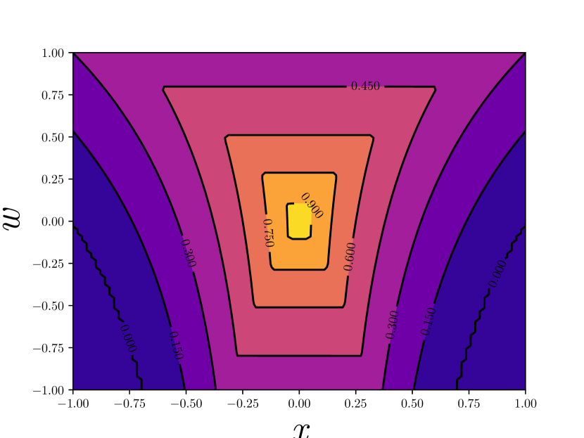
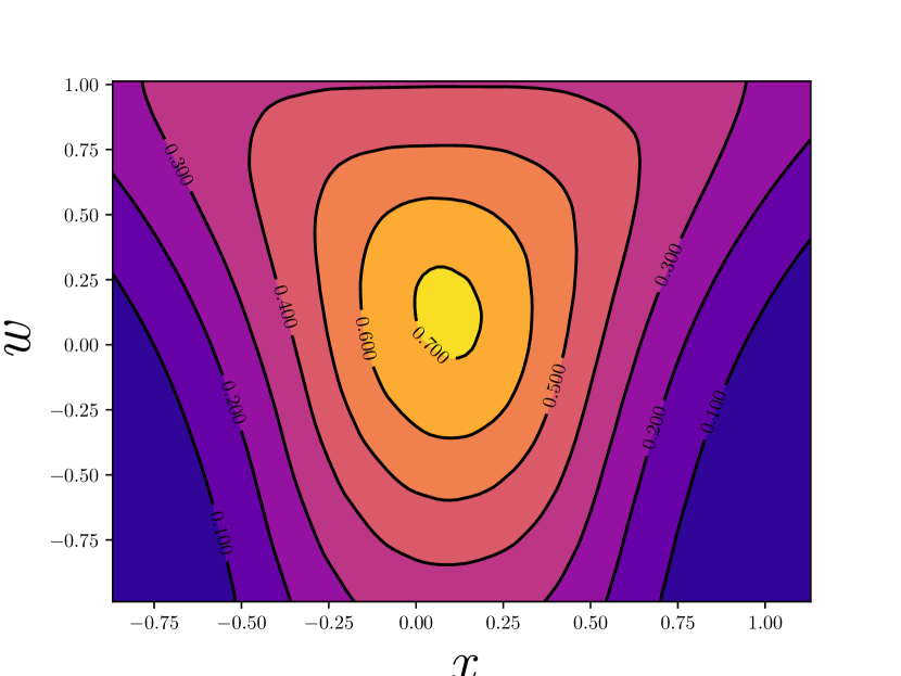
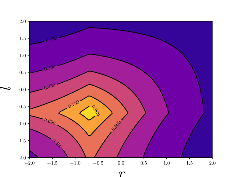
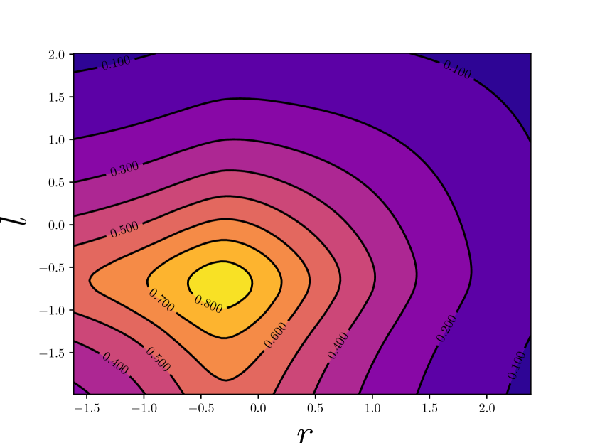
Although the form of positive likelihood is similar to that in [45], we replace the localization term with the IoU that is used in . This is due to three facts. First, the IoU loss has shown relatively better performance, as in UnitBox [38]. Second, IoU is hyperparameter-free and can be considered as a non-parametric localization likelihood. Third, from the perspective of optimization, the IoU loss is more compatible to our proposed method. In Figure 3 we show the variational effect on gradient from localization regression. By applying variational inference, we properly smooth the gradient at some angular points, making the learning process more stable. Experiments in section 4 also suggest that when IoU loss and variational detector are used together, our method achieves better results for crowded pedestrian detection.
Negative pseudo likelihood cannot be directly constructed by sampling ground truth boxes from the dataset. It is necessary to involve a probabilistic negative sample mining procedure for efficiency consideration.
We define , which corresponds to the precision likelihood in [45]. Hence, represents the probability of failing to suppress the negative proposal . The maximum likelihood method implies binary cross-entropy loss for dense proposal . However, recent studies [19, 3, 33, 43] show that single-stage detectors optimized by cross-entropy loss suffer from extreme foreground and background imbalance which results in poor performance. To handle this problem, Focal loss [19] remains one of the state-of-the-art methods.
In this paper, we reformulate Focal loss [19] as a probabilistic online hard example mining [33] method to obtain negative samples for computing the negative likelihood. Recall that not all boxes will be counted as negative samples in the final detection since (1) low-score boxes are usually ignored in practice; (2) ranking based metrics like average precision (AP) are more sensitive to high-score boxes. Formally, we introduce an independent auxiliary Bernoulli random variable with parameter . We choose to include as a negative sample if and only if . Thus, the negative likelihood is:
| (9) |
By designing the probability to keep the dense proposal as , the negative pseudo likelihood is reduced to the Focal Loss [19]. A detailed proof is provided in the Appendix.
The final pseudo detection log-likelihood is given by combining Equation 8 and Equation 9:
| (10) |
where the factors , and are kept the same as in [45].
4 Experiments
4.1 Implementation details
Backbone. We adopt the RetinaNet [19] architecture with ResNet-50-FPN [18, 13] backbone. Following ATSS [42], we define one anchor per pixel for simplicity. We present experimental results on FA [45] and FCOS [35]. FA is an anchor-based method of which the four regression variables for the center-point location, width and height are predicted to recover the box. FCOS is an anchor-free method and its regression targets are distances from the location to four sides of the bounding box.
Training details. We implement the AEVB algorithm in the mmdetection [2] framework. Pedestrian detection methods are compared on two widely used datasets including the CrowdHuman [32] and the CityPersons [41, 7] datasets. The Crowdhuman consists of 15,000 images with 339,565 human instances for training, and 4,370 images for validation. For CityPersons, we train our models on 2,112 images in the reasonable (R) and highly occluded (HO) subsets, and evaluate on 500 images in the validation set. All experiments are conducted on challenging full-body annotations.
We apply SGD optimizer with an initial learning rate , momentum , and weight decay . For the CrowdHuman dataset, we train our models on GTX 1080Ti GPUs with images per GPU for epochs and the learning rate is then reduced by an order at the and epochs. For fair comparison with the RetinaNet baseline on CrowdHuman, multi-scale training and testing are not applied. We resize the short edges of input images to 800 pixels while long edges are kept less than 1333. For CityPersons dataset, we follow the data augmentation setup in Pedestron [12], applying images per GPU on GTX 1080Ti GPUs. The training schedule and learning rate is doubled to that of CrowdHuman setup. The image size for testing is kept the same as the original i.e. .
We choose univariate normal distribution as the variational distribution family for the four localization variables. In total, nine variables are predicted for each anchor: one for classification, four for mean , and four for standard deviation . The standard deviation is necessary for training but not considered during the inference procedure since the final detection boxes take the maximum likelihood (as for normal distribution) at the means.
Evaluation metric. We apply log average miss rate (MR) proposed in [8], which is the average miss rate in log scale over false-positives per image ranging from . A lower miss rate indicates better detection performance.
4.2 Main result
Comparison to the state-of-the-art. On both the CrowdHuman [32] and CityPersons [41, 7] datasets, we compare the AEVB optimized single-stage detectors to (1) its plain maximum likelihood counterpart (i.e. FreeAnchor baseline); (2) state-of-the-art general-purpose single-stage object detector RetinaNet [19, 32] and RFB-Net [20] with offline anchor assignment; (3) representative two-stage methods: Faster R-CNN [29] and Adaptive-NMS [21].
We focus on the popular benchmark CrowdHuman for pedestrian detection and most of the comparisons and ablations are conducted on it. Several conclusions can be drawn from Table 1 (1) Our method is far in excess of the offline learning methods RFB Net and RetinaNet. (2) The average miss rate of FreeAnchor and FCOS drop from to and from to if optimized by our method. (3) Our optimized two-stage solution Faster R-CNN based on [21] obtains better miss rate compared to the state-of-the-art Adaptive-NMS method. (4) We execute our method on a new Faster R-CNN baseline implemented by [6] and improve the miss rate up to in comparison to OP-MP[6] with miss rate, which brings the state-of-the-art to a new bar.
We also extend our method to another widely used benchmark CityPersons. Accroding to Table 2, our method outperforms the plain single-stage method RetinaNet, RFB-Net and TLL in crowd detection on CityPersons. The average miss rate of FreeAnchor drops from to on the CityPersons reasonable subset and from to on the highly occluded subset by using our method. As for the two-stage detectors, we verify the superiority of our method over other two-stage methods including Repp Loss [36] and Adaptive-NMS [21]. These results indicate that learning-to-match with the AEVB algorithm outperforms plain maximum likelihood methods on both datasets.
| Method | MR | |
|---|---|---|
| Single-stage | RFB Net [20, 21] | 65.2 |
| RetinaNet [19, 32] | 63.3 | |
| FreeAnchor () | 52.8 | |
| FCOS () | 48.3 | |
| FreeAnchor () | 50.7 | |
| FCOS () | 47.7 | |
| Two-stage | Faster R-CNN () | 52.4 |
| Faster R-CNN () | 51.2 | |
| Adaptive NMS [21] | 49.7 | |
| Faster R-CNN () | 48.8 | |
| Faster R-CNN () | 42.9 | |
| Faster R-CNN () | 42.4 | |
| GossipNet [14] | 49.4 | |
| RelationNet [15] | 48.2 | |
| OP-MP [6] | 41.4 | |
| Faster R-CNN () | 40.7 |
| Method | R | HO | |
| Single-stage | RetinaNet [19, 12] | 15.6 | 49.9 |
| FreeAnchor | 14.8 | 42.8 | |
| TLL [34] | 14.4 | 52.0* | |
| RFB Net [20, 21] | 13.9 | - | |
| FreeAnchor() | 13.6 | 41.5 | |
| Two-stage | Faster R-CNN [36] | 14.6 | 60.6* |
| Rep Loss [36] | 13.2 | 56.9* | |
| Adaptive-NMS [21] | 12.9 | 56.4* | |
| Faster R-CNN () | 12.7 | 54.6* |
* denotes the detector is not trained on the HO subset.
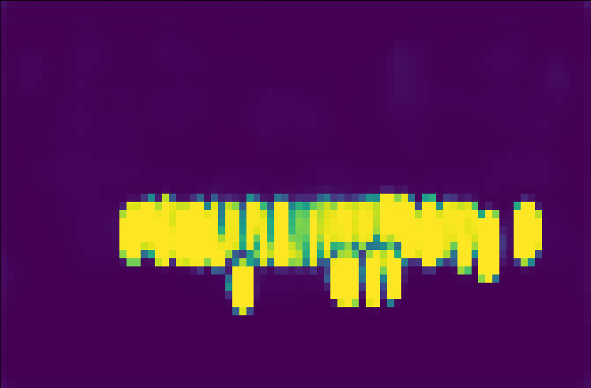
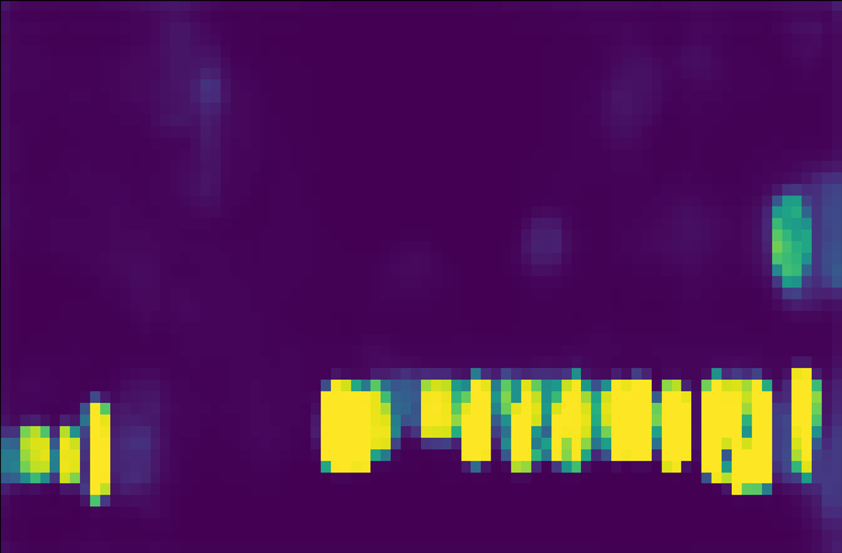
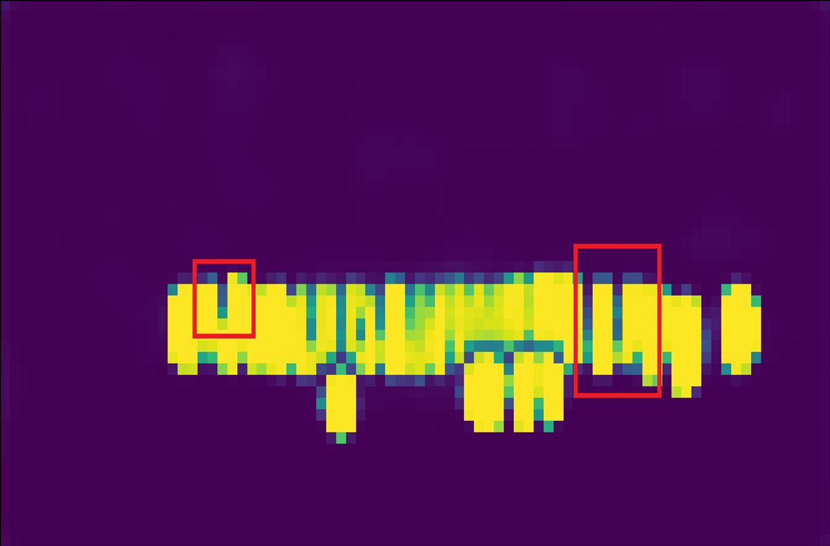
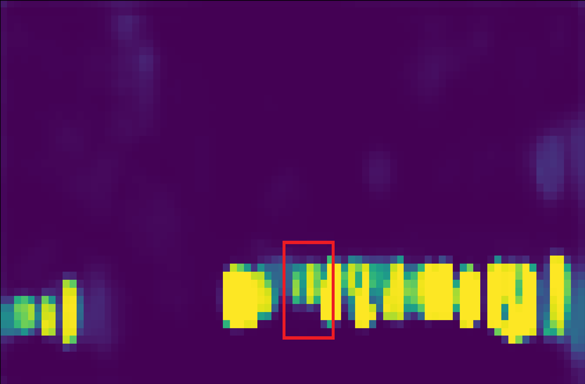
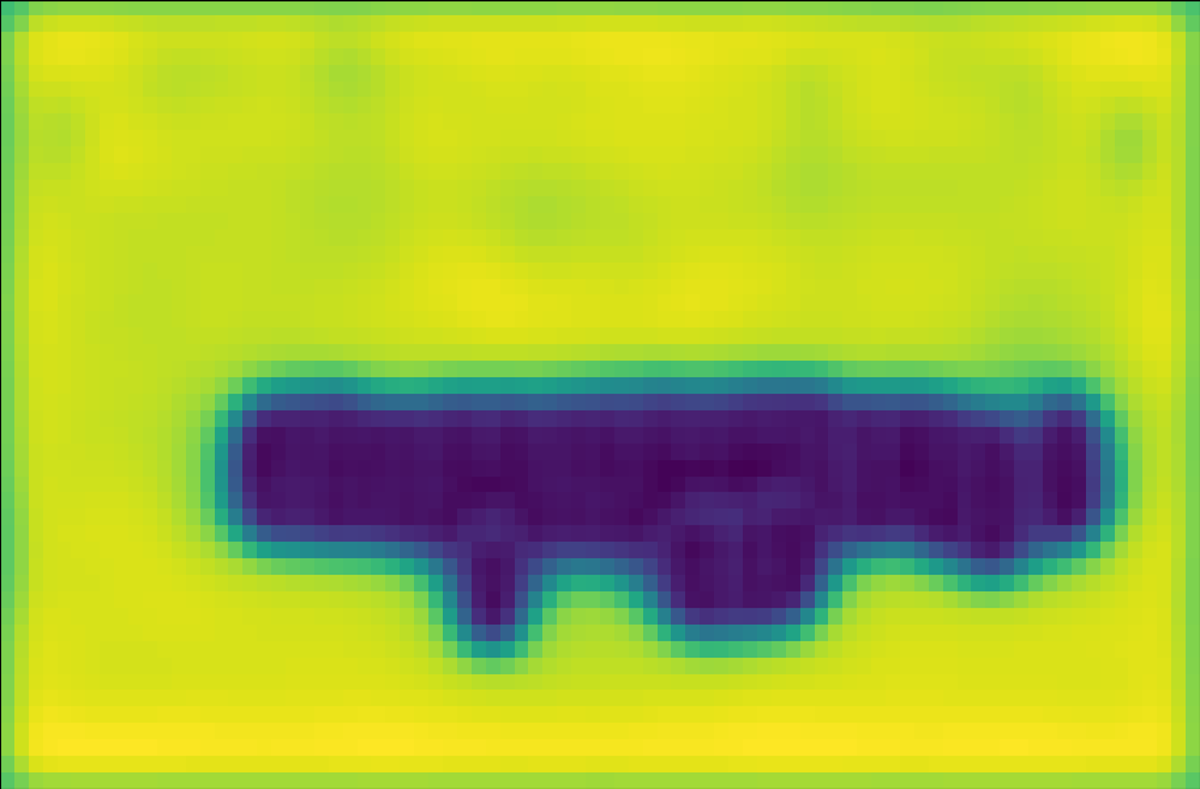
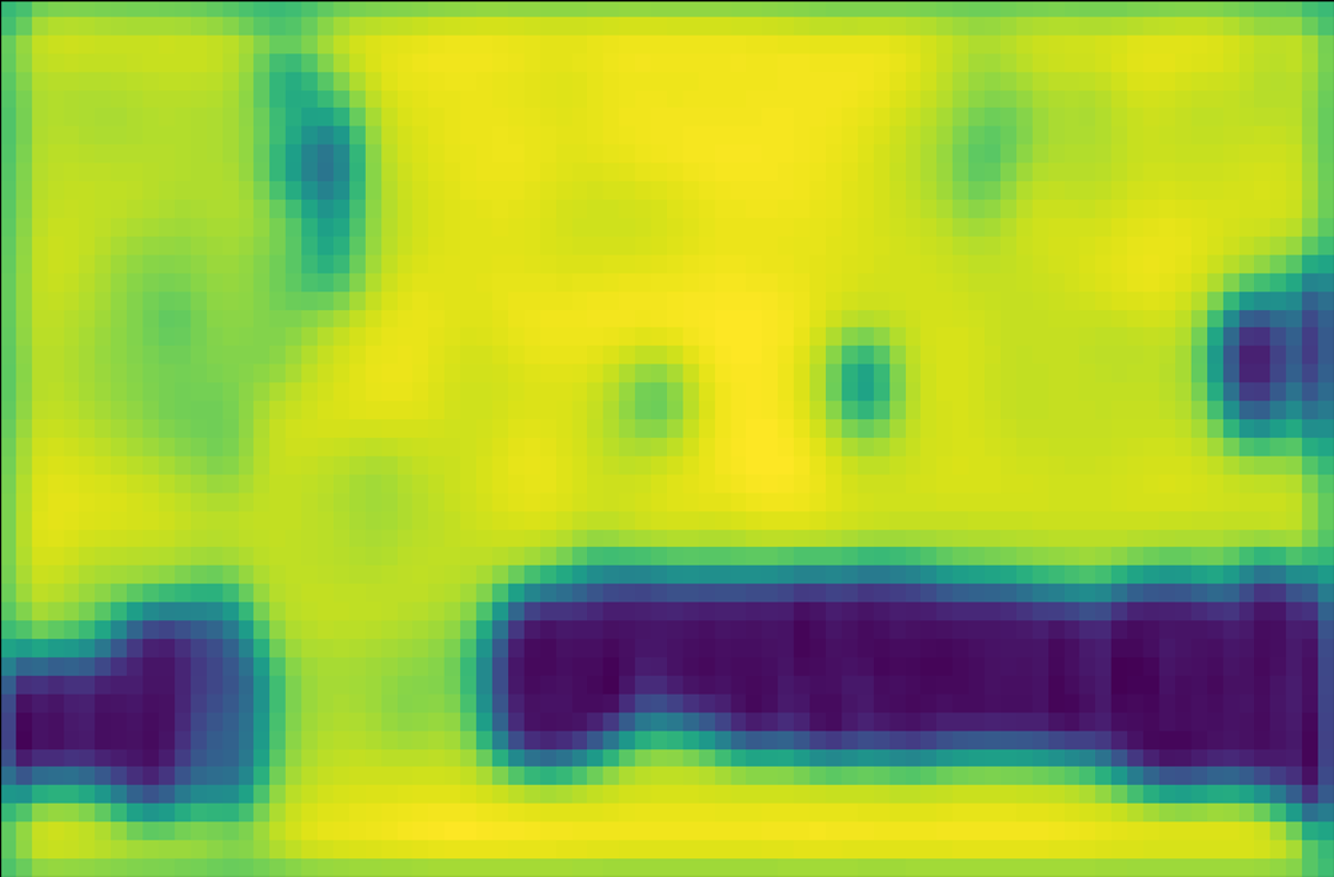
Relation between score and variance. We show the score map and variance map learned by the AEVB algorithm in comparison to the maximum likelihood method in Figure 4. For fairness, single anchor design and IoU likelihood are applied in both methods. The score map learned by AEVB (4(c)) shows a more compact assignment and a cleaner background compared to the score map optimized by ML (4(b)). Furthermore, we plot the variance map in 4(d) as the sum of log standard deviation, i.e., . Intuitively, the variance is closer to one for background pixels due to KL regularization (1st term in Equation 2) while it is significantly lower for foreground pixels due to the data term (2nd term in Equation 2).
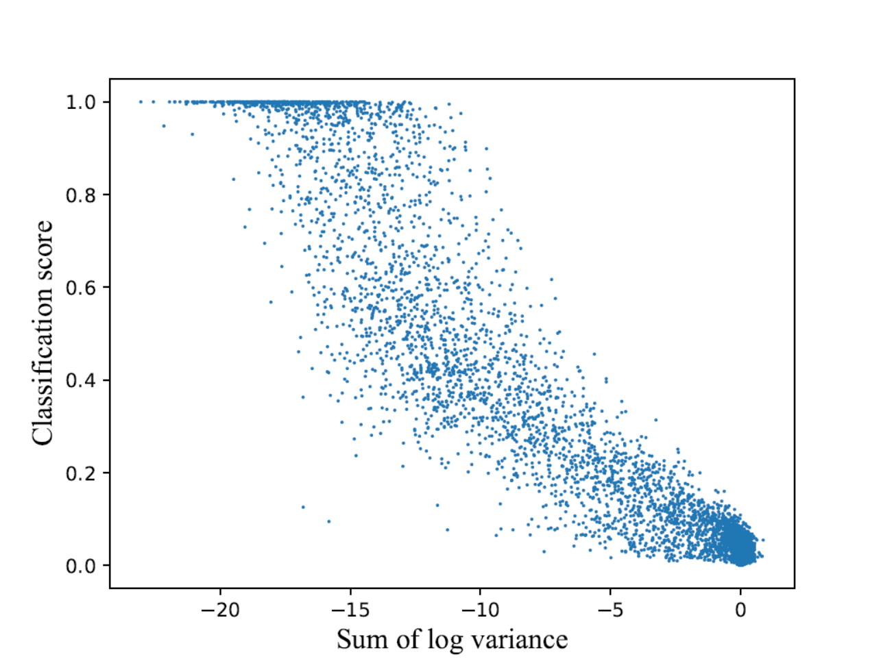
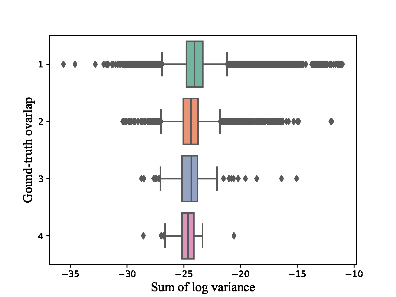
We also visualize the predicted variance of dense proposals versus their classification score and overlap with groundtruth respectively. In 5(a), proposals with low confidence ususally yield large variance to encourage a broader searching space for potential matched ground-truth boxes, while most confident proposals keep low variance to ensure stable regression. 5(b) shows that the median of proposal variance and the number of proposals with large variance outlier decrease as the number of matched ground-truth boxes increases. Thus, our method can be termed as occlusion-aware. These phenomenons not only help to stabilize the optimization in dense crowd region, but also improve the miss rate.
4.3 Ablation study
Detection pipelines. As analyzed in subsection 3.4, our method can smooth the IoU gradient map, facilitating a more feasible gradient descent. We verify our hypothesis in Table 3. It shows that the effect of using IoU loss is quite notable (1.22%) and adding AEVB to detectors based on IoU loss further enhances the detection performance (0.94%). Likewise, FCOS with our approach improves MR by 0.74% over its baseline. Based on these results, we can conclude that both the variational dense proposal and IOU-based detection extraction module jointly improve the performance over occluded scenes. Moreover, our method can generalize well to both anchor-based and anchor-free methods.
| Method | IoU loss | AEVB | MR |
|---|---|---|---|
| FA () | 52.83 | ||
| FA () | ✓ | 51.61 | |
| FA () | ✓ | ✓ | 50.67 |
| FCOS () | ✓ | 48.31 | |
| FCOS () | ✓ | ✓ | 47.57 |
The KL factor. The scaling factor can be tuned to match the pseudo detection likelihood . We tested our algorithm on the CrowdHuman [32] dataset with scaling factors ranging from to . Results in Table 4 indicate that yields the best performance with our algorithm outperforming the plain maximum likelihood method (FreeAnchor + IoU) on the CrowdHuman dataset by 0.94% MR. Note that this value is also a stable choice for the CityPerson dataset. The best values of KL factor for FCOS and Faster R-CNN are nearly the same () which implies that the optimal setting of is not sensitive to concrete box models.
| KL factor | |||
|---|---|---|---|
| FreeAnchor() | 51.96 | 51.27 | 50.67 |
| FCOS() | 47.78 | 47.57 | 48.69 |
| Faster R-CNN() | 40.93 | 40.69 | 41.19 |
The number of anchors. The results in Table 5 shows that the effect of increasing the number of anchors sample is non-negligible. FreeAnchor with two-anchor design can enhance the MR by 0.36% while four-anchor design further improve it by 0.38%. FCOS with four-anchor design can achieve a 0.08% improvement. The training time consumption of both methods increase by about 8% compared to the baselines. And their multiple-anchor designs only incur acceptable addition of training runtime. The testing runtime is not affected as we directly take the mean of each variable as the final localization results, following max-likelihood principle. Qualitatively, single-anchor design are sufficient for good performance while being more efficient with multiple-anchor design. However, considering simpler design and faster training, we keep to the single anchor design for all other reporting.
| Method | anchor(s) | MR | training time |
|---|---|---|---|
| FreeAnchor() | 52.83 | 8.06 h | |
| FreeAnchor() | 50.67 | 8.63 h | |
| 50.31 | 9.77 h | ||
| 49.93 | 11.91 h | ||
| FCOS() | 47.57 | 10.88 h | |
| 47.49 | 12.53 h |
Levels of occlusion. The human instances in CrowdHuman dataset are split into 3 subsets according to the level of occlusion, i.e., the maximum IoU to other human instances. Table 6 shows that the AEVB algorithm outperforms the offline method RetinaNet and online method FreeAnchor across all levels of occlusion especially on the Partial subset where the intra-class occlusion is still reasonably highThe overall detection performance on the Heavy occlusion subset is expectantly poorer than the other subsets, but improvements are noticeable as well with AEVB.
| Occlusion | Bare | Partial | Heavy | All |
|---|---|---|---|---|
| IoU | ||||
| # instances | 47469 | 49146 | 2866 | 99481 |
| RetinaNet | 54.50 | 59.39 | 65.69 | 59.97 |
| FA() | 49.32 | 57.15 | 66.48 | 52.83 |
| FA() | 47.83 | 52.97 | 65.15 | 51.61 |
| FA() | 46.91 | 52.19 | 64.32 | 50.67 |
4.4 Extension to two-stage methods
Although we mainly focus on single-stage pedestrian detection, the proposed optimization algorithm can be flexibly extended to two-stage methods. We applied the proposed AEVB algorithm to optimize the RPN in Faster R-CNN [29] while leaving the network structure and the second stage unchanged. Table 1 and Table 2 list the experimental results on both evaluated datasets, which show Faster R-CNN + AEVB clearly outperforms the original Faster R-CNN and its extensions [6, 14, 15, 21]. This verifies the generalization capability of the proposed AEVB algorithm.
5 Conclusion
We reformulate single-stage pedestrian detection as a variational inference problem and propose a customized Auto-Encoding Variational Bayes (AEVB) algorithm to optimize the problem. For the determination of intractable detection likelihood, we provide a relaxed solution which works well on both FreeAnchor and FCOS box models. We demonstrate the potential of this formulation to propel pedestrian detection performance of single-stage detectors to higher level, while showing that the proposed optimization can also be generalized to two-stage detectors.
Acknowledgement. The paper is supported in part by the following grants: China Major Project for New Generation of AI Grant (No.2018AAA0100400), National Natural Science Foundation of China (No. 61971277).
References
- [1] Florian Chabot, Mohamed Chaouch, and Quoc Cuong Pham. Lapnet : Automatic balanced loss and optimal assignment for real-time dense object detection. arXiv preprint arXiv:1911.01149, 2019.
- [2] Kai Chen, Jiaqi Wang, Jiangmiao Pang, Yuhang Cao, Yu Xiong, Xiaoxiao Li, Shuyang Sun, Wansen Feng, Ziwei Liu, Jiarui Xu, Zheng Zhang, Dazhi Cheng, Chenchen Zhu, Tianheng Cheng, Qijie Zhao, Buyu Li, Xin Lu, Rui Zhu, Yue Wu, Jifeng Dai, Jingdong Wang, Jianping Shi, Wanli Ouyang, Chen Change Loy, and Dahua Lin. Mmdetection: Open mmlab detection toolbox and benchmark. arXiv preprint arXiv:1906.07155, 2019.
- [3] Kean Chen, Jianguo Li, Weiyao Lin, John See, Ji Wang, Lingyu Duan, Zhibo Chen, Changwei He, and Junni Zou. Towards accurate one-stage object detection with ap-loss. In Proceedings of CVPR, pages 5119–5127, 2019.
- [4] Cheng Chi, Shifeng Zhang, Junliang Xing, Zhen Lei, Stan Li, and Xudong Zou. Pedhunter: Occlusion robust pedestrian detector in crowded scenes. In AAAI 2020 : The Thirty-Fourth AAAI Conference on Artificial Intelligence, 2020.
- [5] Cheng Chi, Shifeng Zhang, Junliang Xing, Zhen Lei, Stan Li, and Xudong Zou. Relational learning for joint head and human detection. In AAAI 2020 : The Thirty-Fourth AAAI Conference on Artificial Intelligence, 2020.
- [6] Xuangeng Chu, Anlin Zheng, Xiangyu Zhang, and Jian Sun. Detection in crowded scenes: One proposal, multiple predictions. arXiv preprint arXiv:2003.09163, 2020.
- [7] Marius Cordts, Mohamed Omran, Sebastian Ramos, Timo Rehfeld, Markus Enzweiler, Rodrigo Benenson, Uwe Franke, Stefan Roth, and Bernt Schiele. The cityscapes dataset for semantic urban scene understanding. In 2016 IEEE Conference on Computer Vision and Pattern Recognition (CVPR), pages 3213–3223, 2016.
- [8] P. Dollar, C. Wojek, B. Schiele, and P. Perona. Pedestrian detection: An evaluation of the state of the art. IEEE Transactions on Pattern Analysis and Machine Intelligence, 34(4):743–761, 2012.
- [9] Ross Girshick. Fast r-cnn. In 2015 IEEE International Conference on Computer Vision (ICCV), pages 1440–1448, 2015.
- [10] Ross Girshick, Jeff Donahue, Trevor Darrell, and Jitendra Malik. Rich feature hierarchies for accurate object detection and semantic segmentation. In CVPR ’14 Proceedings of the 2014 IEEE Conference on Computer Vision and Pattern Recognition, pages 580–587, 2014.
- [11] Peter W. Glynn. Likelihood ratio gradient estimation for stochastic systems. Communications of The ACM, 33(10):75–84, 1990.
- [12] Irtiza Hasan, Shengcai Liao, Jinpeng Li, Saad Ullah Akram, and Ling Shao. Pedestrian detection: The elephant in the room. arXiv preprint arXiv:2003.08799, 2020.
- [13] Kaiming He, Xiangyu Zhang, Shaoqing Ren, and Jian Sun. Deep residual learning for image recognition. In 2016 IEEE Conference on Computer Vision and Pattern Recognition (CVPR), pages 770–778, 2016.
- [14] Jan Hosang, Rodrigo Benenson, and Bernt Schiele. Learning non-maximum suppression. In 2017 IEEE Conference on Computer Vision and Pattern Recognition (CVPR), pages 6469–6477, 2017.
- [15] Han Hu, Jiayuan Gu, Zheng Zhang, Jifeng Dai, and Yichen Wei. Relation networks for object detection. In 2018 IEEE/CVF Conference on Computer Vision and Pattern Recognition, pages 3588–3597, 2018.
- [16] Diederik P Kingma and Max Welling. Auto-encoding variational bayes. In ICLR 2014 : International Conference on Learning Representations (ICLR) 2014, 2014.
- [17] Hei Law and Jia Deng. Cornernet: Detecting objects as paired keypoints. International Journal of Computer Vision, 128(3):642–656, 2020.
- [18] Tsung-Yi Lin, Piotr Dollar, Ross Girshick, Kaiming He, Bharath Hariharan, and Serge Belongie. Feature pyramid networks for object detection. In 2017 IEEE Conference on Computer Vision and Pattern Recognition (CVPR), pages 936–944, 2017.
- [19] Tsung-Yi Lin, Priya Goyal, Ross Girshick, Kaiming He, and Piotr Dollar. Focal loss for dense object detection. IEEE Transactions on Pattern Analysis and Machine Intelligence, 42(2):318–327, 2020.
- [20] Songtao Liu, Di Huang, and Yunhong Wang. Receptive field block net for accurate and fast object detection. In Proceedings of the European Conference on Computer Vision (ECCV), pages 404–419, 2018.
- [21] Songtao Liu, Di Huang, and Yunhong Wang. Adaptive nms: Refining pedestrian detection in a crowd. In 2019 IEEE/CVF Conference on Computer Vision and Pattern Recognition (CVPR), pages 6459–6468, 2019.
- [22] Wei Liu, Dragomir Anguelov, Dumitru Erhan, Christian Szegedy, Scott E. Reed, Cheng-Yang Fu, and Alexander C. Berg. Ssd: Single shot multibox detector. european conference on computer vision, pages 21–37, 2016.
- [23] Wei Liu, Shengcai Liao, Weidong Hu, Xuezhi Liang, and Xiao Chen. Learning efficient single-stage pedestrian detectors by asymptotic localization fitting. In Proceedings of the European Conference on Computer Vision (ECCV), pages 643–659, 2018.
- [24] Wei Liu, Shengcai Liao, Weiqiang Ren, Weidong Hu, and Yinan Yu. High-level semantic feature detection: A new perspective for pedestrian detection. In 2019 IEEE/CVF Conference on Computer Vision and Pattern Recognition (CVPR), pages 5187–5196, 2019.
- [25] Yang Liu, Xu Tang, Xiang Wu, Junyu Han, Jingtuo Liu, and Errui Ding. Hambox: Delving into online high-quality anchors mining for detecting outer faces. arXiv preprint arXiv:1912.09231, 2019.
- [26] Ruiqi Lu and Huimin Ma. Semantic head enhanced pedestrian detection in a crowd. arXiv preprint arXiv:1911.11985, 2019.
- [27] Joseph Redmon, Santosh Divvala, Ross Girshick, and Ali Farhadi. You only look once: Unified, real-time object detection. In 2016 IEEE Conference on Computer Vision and Pattern Recognition (CVPR), pages 779–788, 2016.
- [28] Joseph Redmon and Ali Farhadi. Yolov3: An incremental improvement. arXiv preprint arXiv:1804.02767, 2018.
- [29] Shaoqing Ren, Kaiming He, Ross Girshick, and Jian Sun. Faster r-cnn: Towards real-time object detection with region proposal networks. IEEE Transactions on Pattern Analysis and Machine Intelligence, 39(6):1137–1149, 2017.
- [30] Francisco J. R. Ruiz, Michalis K. Titsias, and David M. Blei. The generalized reparameterization gradient. In NIPS’16 Proceedings of the 30th International Conference on Neural Information Processing Systems, pages 460–468, 2016.
- [31] Tim Salimans and David A. Knowles. Fixed-form variational posterior approximation through stochastic linear regression. Bayesian Analysis, 8(4):837–882, 2013.
- [32] Shuai Shao, Zijian Zhao, Boxun Li, Tete Xiao, Gang Yu, Xiangyu Zhang, and Jian Sun. Crowdhuman: A benchmark for detecting human in a crowd. arXiv preprint arXiv:1805.00123, 2018.
- [33] Abhinav Shrivastava, Abhinav Gupta, and Ross Girshick. Training region-based object detectors with online hard example mining. In 2016 IEEE Conference on Computer Vision and Pattern Recognition (CVPR), pages 761–769, 2016.
- [34] Tao Song, Leiyu Sun, Di Xie, Haiming Sun, and Shiliang Pu. Small-scale pedestrian detection based on topological line localization and temporal feature aggregation. In Proceedings of the European Conference on Computer Vision (ECCV), pages 554–569, 2018.
- [35] Zhi Tian, Chunhua Shen, Hao Chen, and Tong He. Fcos: Fully convolutional one-stage object detection. In 2019 IEEE/CVF International Conference on Computer Vision (ICCV), pages 9626–9635, 2019.
- [36] Xinlong Wang, Tete Xiao, Yuning Jiang, Shuai Shao, Jian Sun, and Chunhua Shen. Repulsion loss: Detecting pedestrians in a crowd. arXiv preprint arXiv:1711.07752, 2017.
- [37] Ronald J. Williams. Simple statistical gradient-following algorithms for connectionist reinforcement learning. Machine Learning, 8(3):229–256, 1992.
- [38] Jiahui Yu, Yuning Jiang, Zhangyang Wang, Zhimin Cao, and Thomas Huang. Unitbox: An advanced object detection network. In Proceedings of the 24th ACM international conference on Multimedia, pages 516–520, 2016.
- [39] Kevin Zhang, Feng Xiong, Peize Sun, Li Hu, Boxun Li, and Gang Yu. Double anchor r-cnn for human detection in a crowd. arXiv preprint arXiv:1909.09998, 2019.
- [40] Liliang Zhang, Liang Lin, Xiaodan Liang, and Kaiming He. Is faster r-cnn doing well for pedestrian detection? In European Conference on Computer Vision, pages 443–457, 2016.
- [41] Shanshan Zhang, Rodrigo Benenson, and Bernt Schiele. Citypersons: A diverse dataset for pedestrian detection. In 2017 IEEE Conference on Computer Vision and Pattern Recognition (CVPR), pages 4457–4465, 2017.
- [42] Shifeng Zhang, Cheng Chi, Yongqiang Yao, Zhen Lei, and Stan Z. Li. Bridging the gap between anchor-based and anchor-free detection via adaptive training sample selection. arXiv preprint arXiv:1912.02424, 2019.
- [43] Shifeng Zhang, Longyin Wen, Xiao Bian, Zhen Lei, and Stan Z. Li. Single-shot refinement neural network for object detection. arXiv preprint arXiv:1711.06897, 2017.
- [44] Shifeng Zhang, Longyin Wen, Xiao Bian, Zhen Lei, and Stan Z. Li. Occlusion-aware r-cnn: Detecting pedestrians in a crowd. In Proceedings of the European Conference on Computer Vision (ECCV), pages 637–653, 2018.
- [45] Xiaosong Zhang, Fang Wan, Chang Liu, Rongrong Ji, and Qixiang Ye. Freeanchor: Learning to match anchors for visual object detection. In NeurIPS 2019 : Thirty-third Conference on Neural Information Processing Systems, pages 147–155, 2019.