11email: {anindyag,angshuman,nitin}@cse.iitk.ac.in
VDOO: A Short, Fast, Post-Quantum Multivariate Digital Signature Scheme
Abstract
Hard lattice problems are predominant in constructing post-quantum cryptosystems. However, we need to continue developing post-quantum cryptosystems based on other quantum hard problems to prevent a complete collapse of post-quantum cryptography due to a sudden breakthrough in solving hard lattice problems. Solving large multivariate quadratic systems is one such quantum hard problem.
Unbalanced Oil-Vinegar is a signature scheme based on the hardness of solving multivariate equations. In this work, we present a post-quantum digital signature algorithm VDOO (Vinegar-Diagonal-Oil-Oil) based on solving multivariate equations. We introduce a new layer called the diagonal layer over the oil-vinegar-based signature scheme Rainbow. This layer helps to improve the security of our scheme without increasing the parameters considerably. Due to this modification, the complexity of the main computational bottleneck of multivariate quadratic systems i.e. the Gaussian elimination reduces significantly. Thus making our scheme one of the fastest multivariate quadratic signature schemes. Further, we show that our carefully chosen parameters can resist all existing state-of-the-art attacks. The signature sizes of our scheme for the National Institute of Standards and Technology’s security level of I, III, and V are 96, 226, and 316 bytes, respectively. This is the smallest signature size among all known post-quantum signature schemes of similar security.
Keywords:
Post-quantum Digital signature Multivariate Cryptography Oil-Vinegar Multivariate root-finding1 Introduction
Cryptography is the study of different methods to safeguard our sensitive information in the ever-expanding digital world. The security assurances of cryptographic schemes especially public-key cryptographic schemes emanate from the computational intractability of some underlying hard problems. Currently, public-key cryptographic schemes such as Rivest-Shamir-Adleman [51], elliptic-curve discrete logarithm [44] are predominant in our public-key infrastructure. However, in the context of the rapid development of quantum computers, these schemes exhibit a significant drawback. The underlying hard problems of these schemes i.e. integer factorization and discrete logarithm problem can be solved easily due to the polynomial time quantum algorithms developed by Shor [54] and Proos-Zalka [50] respectively. Therefore, quantum-resistant hard problems have gained popularity among designers for designing public-key cryptosystems for the future. A landmark event in the development of such quantum-resistant or post-quantum cryptography (PQC) is the PQC standardization procedure [19] initiated by the National Institute of Standards and Technology (NIST) to select quantum-safe cryptographic primitives such as key encapsulation mechanisms (KEM), public-key encryption (PKE), and digital signature algorithm. In 2022, NIST standardized [3] one KEM (Crystals-Kyber [15]) and three signature schemes (SPHINCS+ [4], Crystals-Dilithium [26], and Falcon [32]) after rigorous scrutiny spanning multiple years. Among these only SPHINCS+ is based on the hardness of cryptographically secure hash functions, while Crystals-Kyber (KEM), Crystals-Dilithium, and Falcon are based on hard lattice problems. As the majority of these constructions are lattice-based, there is a lingering risk that a breakthrough in the cryptanalysis of lattice-based cryptography can reduce the security of these schemes drastically. Thus putting the whole plan to migrate to post-quantum cryptography in jeopardy. Such incidents are not uncommon. Recently, Decru et al. [18] proposed an attack to completely break the security of supersingular isogeny Diffie-Hellman [31] which was earlier considered quantum-safe and was also a finalist in the NIST’s standardization procedure. Therefore, it is prudent to diversify the portfolio of different quantum-safe problems for seamless migration to a post-quantum world. There exist other problems that are considered quantum-safe, such as multivariate quadratic (MQ) [46, 39], isogeny-based [22], and code-based [8]. Standardizing cryptographic primitives necessitates a rigorous and comprehensive investigation. NIST reissued a call [20] for quantum-safe signature schemes to standardize some more signature schemes to diversify the portfolio of quantum-resistant schemes. Due to its small signature size, multivariate oil-vinegar construction has gained significant attention during this standardization process.
Multivariate cryptography relies on the intractability of root findings of MQ equations. The goal of the MQ problem is to find a solution to a system of multivariate quadratic polynomials in the finite field . In other words, the hardness classification of this problem is NP-hard [38]. Numerous schemes, such as Matsumoto-Imai encryption scheme [43], Oil-Vinegar [46] signature, Rainbow [24] signature, Triangular [45, 53, 60] signature, Simple Matrix encryption [56], and Mayo [12], have been developed based on multivariate cryptography. Patarin first proposed the Oil-Vinegar signature [46]. A successful forgery attack was shown by Kipnis and Shamir [40] against this scheme. Further, Kipnis, Patarin, and Goubin upgraded the signature scheme by proposing Unbalanced Oil-Vinegar (UOV) [39].
Rainbow was a third-round NIST candidate [24], which is the first multi-layer construction based on unbalanced oil-vinegar. Therefore, the cryptanalysis of Rainbow has been a well-studied area for the last decade. This resulted in many new novel attacks such as direct attack [6, 27, 28], min-rank attack [14, 6, 7, 5], band-separation attack [25, 57, 55], rectangular min-rank and intersection attack [10]. In 2023, Beullens proposed a cryptanalysis and reduced the security of Rainbow significantly. Rainbow team suggested using the old SL-3 (high security) parameter set as new SL-1 (low security) parameters [36] to mitigate the attack. As Beullens’ attack only applies to the Rainbow structure, therefore building scheme on the top of the oil-vinegar layer is still believed to be secure.
In 2022, Cartor et al. internally perturbed the second layer of Rainbow by mixing oil variables quadratically [17]. However, this mixing significantly increased the signature generation time. Also, parameter sets proposed by designers are not practical in terms of efficiency. Therefore, designing a new signature scheme that can resist the simple attack while being practical, is an interesting open problem.
1.1 Our Contribution and Motivation
In the context of this endeavor, we summarize our contributions below.
-
•
We review related multivariate signature schemes and provide a comprehensive analysis of their design and performance in Section 2.
-
•
We present Vinegar-Diagonal-Oil-Oil (VDOO), a novel multivariate signature scheme based on unbalanced oil and vinegar in Section 3. Compared to other UOV schemes VDOO boasts three primary benefits: simplicity, efficiency, and security (see Sections 4 and 5). To the best of our knowledge, we are the first to introduce a diagonal layer within the UOV framework, demonstrating that it enhances efficiency without compromising security.
-
•
We establish that VDOO effectively withstands all current attacks and outline the EUF-CMA security of our scheme. Through meticulous parameter selection, our findings reveal that it achieves a remarkably compact smallest signature size of 96 bytes (see Sections 4 and 5), contrasting favorably with NIST-standardized post-quantum signatures (Crystals-dilithium [26], Falcon [32], and SPHINCS+ [4]).
1.1.1 Introduction of a new simple design element.
VDOO is a new layer-based construction, which has one diagonal layer and then two UOV layers. We are adding each new variable in the central polynomial one by one diagonally. This offers efficiency. This translates to a reduction of the Gaussian elimination ( 111: Gaussian elimination on a linear system with unknowns and linear equation over .) which is the major computational bottleneck in the signature generation process. Suppose are variables defined over . In our construction, we call first -variables as vinegar variables, next -variables as diagonal variables, then next variables are first-layer oil variables, and last variables are second-layer oil variables. Figure 1 illustrates the distribution of the variables in each layer of the VDOO central polynomial map.
Efficiency. To thwart Beullens’ simple attack [11], the authors of Rainbow increased the parameter set [36], which results in increasing the Gaussian elimination cost. The complexity of Gaussian elimination becomes approximately where and are number of oil variables of Rainbow [24]. In our scheme, we adapt , , and as the new parameters. This adjustment results in a Gaussian elimination complexity of around . To illustrate, consider the signature generation process for security level one (SL-1) parameters [19]: UOV requires , Rainbow requires and , while VDOO needs only and (for further details, refer to Table LABEL:tab:compmul). Consequently, this modification notably improves our scheme’s performance.
Resistance to existing attacks. We comprehensively analyze all possible attacks on multivariate cryptographic schemes against our scheme. In an attempt to recover diagonal variables, potential attackers begin by eliminating the uppermost oil layers. Beullens proposed method [11] facilitates the removal of these layers, aiding attackers. For instance, in order to compromise our round-one parameter set, a straightforward attack necessitates -field operations. Furthermore, Beullens combined this simple attack with the rectangular min-rank attack [10, 11]. In line with previous efforts, we execute this combined attack against our scheme, determining that it requires -field operations to break SL-1 parameter set. Additionally, we conduct the intersection attack and the direct attack on our scheme, both of which exhibit complexities exceeding -field operations. Consequently, these references collectively imply that VDOO appears to withstand all known attacks securely. We also outline the EUF-CMA security of the VDOO scheme.
Small signature size. We present multiple parameters that can withstand the aforementioned attacks. Specifically, our level-one parameters that can provide -bit classical and -bit post-quantum security has a signature size of 96 bytes and public-key size of 238KB (further elaborated in Table 1). This is the smallest signature size among the majority of all multivariate signature schemes (for additional insights, refer to Tables LABEL:tab:compmul and LABEL:tab:compsign).
Roadmap. In the upcoming Section 2 we present a generic construction of multivariate signatures, and some earlier results. Section 3 proposes a new post-quantum multivariate signature scheme called VDOO. The cryptanalysis of our scheme is presented in Section 4. In Section 5, we give the parameters for different security levels and we also compare our results with the state-of-the-art. Our section 6 presents conclusions and explores potential future directions for our work.
2 Prior Results
In this section, we introduce some essential mathematical notations and symbols. We then provide a generic construction for multivariate signatures. Following that, we outline the central polynomial for UOV and Rainbow [39, 13, 24]. Additionally, we describe the subspace representation of Rainbow [10], which is particularly valuable for cryptanalysis purposes. Next, we cover recent multivariate signature schemes [12, 34, 29, 23, 33] that were submitted as part of the NIST additional round for post-quantum signature standardization [20]. Finally, we present the required hardness assumptions for these multivariate signatures to understand their cryptanalysis.
Notations. Let, be the finite field with elements. We define two invertible affine maps and , and one quadratic map . We denote for the set and denotes . We use lowercase and bold lowercase alphabets to denote field elements and vectors respectively. The notation is used to interpret is a random element in the set .
2.1 Generic Multivariate Signature Schemes
Here we briefly describe a generic construction for multivariate signature schemes. Due to the NP-hardness of inverting a randomly generated quadratic system [38]. However, signers can leverage a specially structured quadratic system to efficiently perform the inversion. This specialized system is commonly referred to as the central map and is typically denoted as , where each represents a specifically structured multivariate quadratic polynomial. Signers must conceal this unique structure from third parties to prevent forgery attacks. To achieve this objective, signers employ one or two random invertible linear maps: and . Consequently, the public key is constructed by composing these linear maps along with the central map, denoted as .
The secret key comprises and . A hash function, denoted as , is employed to generate a vector from a message . The signature generation process unfolds as follows: first, compute , then , and finally . The signer sends the signature for the message to the verifier. The verifier simply evaluates the polynomial map on and checks whether it matches the hash of the message, i.e., whether holds or not.
2.2 Unbalanced Oil-Vinegar (UOV)
The Oil-Vinegar (OV) signature scheme was initially introduced by Patarin [46]. However, due to the Kipnis-Shamir’s [40] invariant subspace attack, this scheme was modified by increasing the number of vinegar variables. This is known as the Unbalanced Oil-Vinegar (UOV) signature scheme [39].
Consider the OV central map, denoted as . Split all variables of into two buckets: the first bucket has first variables representing vinegar, and the second bucket contains next variables representing oil, where and . To create a multivariate quadratic homogeneous polynomial, combine variables involving vinegar vinegar and vinegar oil, while excluding all oil oil terms.
Definition 1 (OV Central Polynomial Map)
A central map is known as OV central polynomial map when each is of the form where , , and .
Notably, if anyone randomly fixes vinegar variables, then the remaining part would be linear in the oil variables. Therefore, the quadratic system reduces to a linear system of linear equations with unknowns.
2.3 Rainbow
Rainbow is a multi-layer variant of UOV [24]. For simplicity consider a two-layer Rainbow. Suppose , where the first variables are vinegar and the next and variables are the first and second layer of oil variables respectively. This can be viewed as a UOV map with variables and oil variables and the next layer variables and oil variables.
Definition 2 (Rainbow Central Polynomial Map)
The mathematical expression for -layer Rainbow central polynomial is as follows.
where for each , elements ,and are taken from ; denotes the layer, and where is the total number of layers in Rainbow.
2.4 Beullens Subspace Description
For a better view of cryptanalysis on Rainbow, Beullens explained the construction of Rainbow via subspaces [10]. Using this description, he derived the simple attack [11]. To elaborate this idea, initially, we define a differential polar form of a polynomial map.
The differential polar map of a polynomial map is denoted by and defined as Note that, we only consider homogeneous quadratic polynomials, so throughout this paper, .
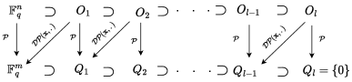
Trapdoor information. This part describes the trapdoor information of -layer Rainbow. At first, signer chooses a secret chain of nested subspaces: input subspaces and output subspaces . Using this secret, one can construct a public polynomial map as follows.
-
•
maps each to and
-
•
for any , is a linear map (see Figure 2)
Inversion. In this methodology, the goal is to compute from given such that . The knowledge of nested sequences of input and output subspaces is used in this computation. At first glance, for -layer Rainbow, the value of the unknown can be represented as where all of the . Fix . Then is used in conjunction with the th-layer’s output subspace to calculate . For the sake of clarity, let’s define the quotient space .
Using the knowledge of sequences of subspaces, the goal is to find for all . This will lead to computing the preimage of any element from . For computing , use the following relation (note that, from definition, ),
Earlier v is fixed, so the quadratic system reduces to a linear system. The number of constraints and variables are the same for the linear system. This implies that a unique solution can be obtained with probability . Repeatedly running this procedure, one can compute all , which implies that preimage will be computed.
In 2022, Beullens [11] reduced the security level of Rainbow. He showed for small , recovering all subspaces is significantly efficient. Also, the small finite field size accelerates the attack.
2.5 Concurrent Proposals
The NIST additional signature submission call [20] received a total of eleven multivariate signature schemes e.g. Mayo [12], QR-UOV [34], TUOV [23], etc. Most of them are based on the old unbalanced Oil-Vinegar structure. For example, Mayo [12] employed a UOV structure along with a new whipped-up MQ (WMQ) approach. QR-UOV is another variant of UOV where the public key is represented by block matrices, with each element corresponding to an element in a quotient ring [34]. Also, in 2022, a new proposal, called IPRainbow [17] was made by perturbing the central polynomials of the second layer by variables. This change although decreases the attack probability by , the running time significantly increases due to the usage of Gröbner basis technique for inversion.
2.6 Hardness of Multivariate Cryptography
Here, we describe other approaches used in the cryptanalysis of multivariate signatures apart from the direct solution of MQ equations.
-
1.
Min-rank. Let be the given matrices and , find a non-trivial linear combination (with ) so that This problem is called the min-rank problem and has been shown to be NP-hard [16]. The min-rank problem appeared as a cryptanalytic tool in multivariate cryptography [41, 30, 6, 10]. This attack helps to find a linear combination of public matrices which sums up to a low-rank matrix.
-
2.
EIP. Find an equivalent composition of , where are equivalent affine maps, and is an equivalent central map. The above problem is the Extended Isomorphism of Polynomials (EIP) problem. No such hardness classification is known (though it subsumes graph isomorphism problem [1, 2]), but for some instances, polynomial time algorithms exist [40].
3 Our Proposal: VDOO Signature Scheme
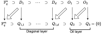
In our scheme, we introduce a new design element called diagonals into the Oil-Vinegar scheme. Let, , we pick the first variables as vinegar variables. We denote the next variables as diagonal variables. In this layer, we introduce quadratic equations. In any -th () equation, only -th variable is unknown among variables. In the following layers, we apply the Oil-Vinegar technique. This means we can generate OV polynomials using -vinegar variables and newly added -oil variables. Further, we construct OV polynomials using -vinegar variables and newly added -oil variables. Finally, we have a quadratic system with variables and homogeneous quadratic equations.
3.1 VDOOSetUp: Generate Parameters
To construct polynomial maps we need to define parameters associated with this. In this phase algorithm takes input the security parameter and output the parameter tuple, that is . Here,
-
•
Finite field which has elements.
-
•
Positive integers and , where denotes the number of vinegar variables, is the number of diagonal variables, and stands for the number of first and second layer oil variables respectively. Therefore, total number of variables is , and number of equations is .
3.2 VDOO Central Polynomial Map and Inversion.
Construction of central polynomial map plays an important role in the multivariate signature schemes. To the best of our knowledge, we are the first to propose a central polynomial map that involves vinegar, diagonal, and oil variables in a three-layer construction.
-
•
Diagonal Layer. Here, we explain the structure of any central polynomial for the diagonal layer . Each is defined as follows.
Each coefficient , and . The subroutine is used to generate such central polynomial in the diagonal layer.
-
•
First Oil Layer. In this oil layer, we use variables as vinegar variables and next variables as oil variables. All these variables help us to construct homogeneous quadratic polynomials of the following form.
where , , and .
-
•
Second Oil Layer. The topmost oil layer has vinegar and oil variables. That means, it has quadratic equations. Those equations are of the form
where and , and . We denote this as to generate a oil-vinegar central polynomial (according to 2.2) which has vinegar variables and oil variables.
Here, Algorithm 1, uses and to generate a VDOO central map .
Inversion. The main computational bottleneck of UOV-based constructions is the inversion of the central polynomial. It requires Gaussian elimination which runs in . However, in our scenario inversion of the diagonal polynomials is straightforward as there is only one unknown variable. Nevertheless, the inversion of OV polynomials in the remaining two layers each needs a Gaussian elimination. Therefore, inverting VDOO central polynomial map needs two Gaussian elimination only. This is shown in Algorithm 2. Following two algorithms help to compute the inverse of the VDOO central polynomial.
-
The subroutine Substitution or converts a bunch of oil-vinegar polynomials to a bunch of linear polynomials consists of oil variables by fixing the vinegar variables. That means, substitutes vinegar variables by random values (in ) in the bunch of oil-vinegar polynomials and converts it to a bunch of linear polynomials of oil variables .
-
The denotes Gaussian elimination for unknowns over the linear system of equations over . It returns a failure when the rank of the matrix representing the linear system is less than .
3.3 VDOOKeyGen: VDOO Key Generation
The in Algorithm 3 generates two random invertible affine maps and along with the VDOO-central map . Here, secret/signing key is , and and public/verification key is the composition map , where . Note that, the individual information of secret maps allows user to compute the inverse of efficiently. We denote to generate a random matrix over from a , helps to compute the inverse of a matrix over , and computes
-
•
Public key: .
-
•
Secret key: , , and .
3.4 VDOOSign: VDOO Signature Generation
Similar to the other OV based constructions [12, 23, 39, 24], we use the hash-and-sign paradigm for our signature algorithm as shown in Algorithm 4. We use a hash function . Signer knows each polynomial map, so it can compute the inverse of each map i.e. , , and . If reports a failure during the computation of , we restart the process by regenerating the salt and repeating the entire procedure. Finally, the signature is computed as .
Efficiency analysis. As mentioned earlier, the major computational overhead of OV-based schemes is the Gaussian elimination procedure. In VDOO, during signing, we have to compute only one Gaussian elimination i.e. computation of . The computation of and can be done during the key-generation procedure. In VDOO the computation of is also very efficient compared to other OV-based schemes as the number of unknowns is smaller in VDOO as shown in Table LABEL:tab:compmul.
3.5 VDOOVerif: VDOO Verification
Our verification procedure is simple. It needs a polynomial evaluation of , requiring just field operations. Compute from public key and signature The signatures is accepted if holds, else rejected.
3.6 Key Size Computation
Our VDOO contains one diagonal layer and two UOV layers. The size of the private key is determined first, followed by the size of the public key.
-
•
Size of the central map for a diagonal layer having -diagonal polynomials is field elements. The first diagonal layer has vinegar variables. In any diagonal layer, a central polynomial has vinegar variables and -th polynomial has vinegar variables.
-
•
Size of the central map for a UOV layer is around field elements. Such UOV layer has vinegar variables and oil variables.
The sizes of the two affine transformations are as follows: for we need , while for we need , field elements. These maps can be generated using a random seed.
3.7 Subspace Description of VDOO Central Polynomial
Our scheme can be explained through Beullens’s subspace descriptions [10]. This description is useful to understand the cryptanalysis of VDOO. In this case, we have input and output subspaces. These sequences of nested subspaces are as follows.
-
•
Input subspaces
-
•
Output subspaces
In the Figure 3 (single arrow denotes and bold arrow denotes ), these following relations will hold: and for . Also, , for . In addition, , .
The signer first fixes . Since , so for diagonal layer computing is very easy. Once these vectors are found, then update . Now, signer needs to solve for , so that the following relation holds. Note that, .
We know that the above equation is a linear system of variables and equations. With the probability , the signer will able to compute . Then signer again updates and follow a similar strategy to find . Thus the signer can finally compute the pre-image of .
4 Security Analysis of VDOO
Cryptanalysis that targets solving the MQ problem directly, is known as the direct attack in multivariate cryptography [6, 27, 28, 9]. Later researchers have used the special structure of the quadratic system and improved the state-of-the-art, like, band-separation attack [25, 57, 55], intersection attack [10], and simple attack [11].
To determine the complexity of the attacks described below by the number of field multiplications required to perform the attack. One -field multiplication needs gates. Here, each -bit stands for one -bit multiplication (represented as AND gates) and the same number of additions (represented as XOR gates) during one -multiplication. Additionally, bits are needed for -bit additions involved in one -addition, which is required for each field multiplication that occurs during an attack. For example, the cost one -multiplication requires 36 gates. Such a strategy to determine the complexity is standard and has been also followed in other MQ-based signature schemes [34, 12, 29].
Henceforth, in this document, we use the parameter set as an example to demonstrate the complexity of the following attacks. Incidentally, this is also our SL-1 parameter. Our full parameter set is given in Table. 1.
4.1 Direct Attack on VDOO
The direct attack is the fundamental methodology for forging any multivariate signature scheme. To counterfeit a VDOO signature, an attacker aims to solve an underdetermined system with variables and homogeneous equations (), to find such that . The basic approach involves converting this underdetermined system into a determined one by fixing variables. Subsequently, quadratic system-solving techniques like the Wiedemann XL algorithm [58, 21] or Gröbner basis methods such as F4 or F5 [27, 28] are applied. Another approach named hybrid approach [9] involves guessing variables prior to solving the system. The time complexity of this attack, using the approach outlined in [9], is expressed in terms of field multiplications as:
Here, denotes the number of variables fixed during the algorithm, and represents the smallest integer for which the coefficient of in the series is non-positive.
Example for SL-1 parameters. Our level one parameter set has 160 variables and 100 constraints. According to [9], we fix 60 variables. Now in the algorithm, if we fix twelve variables, then the value of is 28. The total complexity is around .
4.2 Simple Attack on VDOO
In 2022, Beullens proposed the simple attack against Rainbow [24]. For Rainbow, this highly effective attack reduces -unknown and -constraints in the quadratic system to -unknown and -constraints. Now an attacker can apply the same methodology on VDOO to recover the secret key. Recall from Figure. 3, is the public polynomial map, and sequences of nested input and output subspaces are,
-
•
Input subspaces
-
•
Output subspaces
The main crux of the simple attack lies in finding a vector within (as depicted in Figure. 3). To achieve this, the attacker must solve a quadratic system with unknowns and constraints using the XL algorithm. This computational step constitutes the most significant component of the entire attack. Here is a step-by-step outline detailing the cryptanalysis of our scheme using the simple attack.
- Input:
-
Public polynomial map .
- Output:
-
Recover sequences of subspaces.
- Find a vector :
-
Choose . Then from Figure. 3, is a linear map, in particular it maps to . The attacker uses this linear relation to reduce the number of unknowns present in the quadratic system. Therefore, to find a vector, an attacker should solve the following system.
With probability , the attacker successfully guesses a vector in . Later, the attacker deploys the XL algorithm to solve the quadratic system of -unknowns and -constraints. Thus attacker recovers .
- Recover :
-
Attacker will retrieve using the information . Note that, is a linear map. Therefore,
for some linearly independent vectors . For enough such ’s equality will hold.
- Recover :
-
To recover , solve the following system of linear equations. Because with high probability kernel of matches with .
- Recover a vector :
-
Now the quadratic system reduces to equations and variables. To recover , the goal of the attacker is to find a vector in . Again attacker will guess a vector . Like above, a similar argument shows that is a linear map and the attacker tries to solve the following systems mod .
The attacker runs the XL algorithm to solve the quadratic system of -unknowns and -constraints.
- Recover :
-
Attacks follows same approach as recovering to recover . Here, an attacker solves a system for
- Recovering vectors from diagonal layer:
-
The only task that remains is to find all the diagonal vectors. The attacker can apply Wolf et al.’s [59] trick to find all the diagonal vectors in the layer. Here observe that the computation of finding a vector in , dominates the computation of finding a vector in .
Attack Complexity. The complexity of the first steps dominates the complexity of other steps involved in this algorithm. Basically, a system of variables and non-linear equations reduces to a system of homogeneous equations with variables. This computation can be performed via XL algorithm and it requires
field operations, where is the operating degree of the algorithm. It means, -is the smallest positive integer so that the coefficient of in the power series is non-positive.
Example for SL-1 parameters. Apply Beullens’ trick to guess a vector in , which happens with probability . Finding one vector on asks to solve a quadratic system of -variables 60-unknowns. This computation is the most costly in the entire algorithm. Solving this quadratic system needs field operations. The guessing needs search and cost of one - multiplication needs 36 gates. Therefore, this parameter set provides approximately at-least 128-bit security.
4.3 Rectangular Min-rank Attack on VDOO
Rectangular min-rank attack is proposed by Beullens [10]. We first describe the attack against VDOO and then compute the required attack complexity to perform this attack against VDOO. Attacker starts with -rectangular matrices over where each is defined as
where is a basis of .
Let . The bi-linearity of implies
Hence, the maximum rank of is , since . This observation provides attacker a min-rank instance to find ’s in .
To enhance the performance of the simple attack, Beullens combined the rectangular min-rank attack with the simple attack [11]. Like earlier, the attacker fixes to get a linear map . This helps to find using .
This system of linear equations reduces the number of matrices by in the rectangular min-rank instance. Thus, the basis of Ker( is . Hence, the new min-rank instance has matrices , where
If is a solution of the new min-rank problem having matrices then is a solution of the old min-rank problem. Hence, the attack needs to be repeated approximately times, until it finds .
Attack Complexity. The number of field multiplications required to perform this attack is
where is the operating degree for the algorithm [7].
Example for SL-1 parameters. The attacker needs to guess a good . After then the attacker gets a min-rank instance of 60 matrices which has 159 rows and 100 columns and the span of these matrices has a matrix of rank 36. Bardet et al.’s [7] algorithm provides an efficient way to solve this min-rank instance. This computation needs -field operations.
4.4 Kipnis-Shamir Attack on VDOO
The attacker targeting VDOO can employ a technique similar to the one devised by Kipnis and Shamir [40] to retrieve the subspace . This approach effectively aids in the separation of oil and vinegar variables, ultimately leading to the recovery of the private key. The complexity of this attack can be roughly estimated as field multiplications. To expedite this assault, the attacker leverages Grover’s algorithm, which serves to reduce the complexity to .
Example for SL-1 parameters. Attacker needs to perform approximately -field operations in classical settings and -field operations in quantum computer.
4.5 Intersection Attack on VDOO
Beullens introduced the intersection attack [10], which effectively reduced the claimed security level of the Rainbow signature scheme by approximately 20 bits compared to the original design. In this attack, Beullens improved upon the Rainbow band separation attack [25] using the analysis proposed by Perlner [47]. The intersection attack helps to identify -vectors simultaneously within the oil-space by solving a system of quadratic equations for a vector within the intersection , where ’s are invertible matrices. This attack performs well when the intersection is non-empty, which occurs when . The computational cost of this attack involves solving a quadratic system with equations in variables.
However, in the case of VDOO where , there is no guarantee that the subspace (for more details, see [10]) namely will exist. Consequently, the attack becomes probabilistic for VDOO and will succeed with a probability of .
Example for SL-1 parameters. The complexity to break SL-1 parameters, attacker needs -field multiplications.
4.6 Quantum Attacks
The attacker can accelerate certain aspects of the classical attacks using a quantum computer. For MQ- or OV-based schemes the only quantum algorithm that can help in cryptanalysis is Grover’s search [37]. This algorithm reduces the search space, thereby reducing the number of field multiplications by a factor of . This specifically does not threaten the post-quantum security of our scheme [19].
4.7 Provable security: EUF-CMA Security
Our VDOO scheme, similar to UOV, Rainbow, and other UOV-based signature schemes, offers universal unforgeability [24]. Like these other schemes, we incorporate a salt in the signature generation process to demonstrate the EUF-CMA security of our scheme. We have followed the established methodology for this purpose, as seen in prior work such as [52, 12]. Here, we have only provided an outline of the proof. The full proof can be done using similar strategies as Mayo [12], QR-UOV [34], PROV [29], etc. Our security proof relies on the well-understood hardness of the UOV problem. We begin by defining the UOV problem and then introduce the VDOO problem.
For security reasons, we recommend that each salt value should be used for no more than one signature. Consequently, we fix the salt length at 16 bytes, assuming up to signature generations within the system [19].
Definition 3 (UOV Problem)
Suppose denotes a family of UOV public polynomial maps where is the number variables, is number of equations and is the size of the finite field, and denotes a family of random quadratic systems with unknowns and constraints over . The UOV problem asks to distinguish from and . Suppose be the adversary solves the distinguishing problem and it has a distinguishing advantage as:
It is widely believed that there is no probabilistic polynomial-time adversary, including quantum adversaries, denoted as , that can efficiently solve the UOV problem.
Definition 4 (VDOO Problem)
Suppose be a family of VDOO public polynomial map. Now given a random VDOO problem asks to find such that . If is such an adversary to compute the inverse of the VDOO public map then the advantage of this computation is
Now we are going to state our main theorem which establishes the EUF-CMA security of the VDOO. To understand the security notion, we refer to [12, 52, 42].
Theorem 4.1
Suppose the adversary runs in time to solve the EUF-CMA game of VDOO in the random oracle model. This adversary makes signing queries and random oracle queries. Then there exists and running in time with
Proof idea. Here, we informally sketch the proof. We can adopt the proof methodology used in Mayo (see theorem from [12]). In the first step, we can establish a reduction from the EUF-CMA security of the VDOO signature scheme to EUF-KOA (Existential unforgeability against key-only attack) security by simulating the signing oracle. Note that, the adversary does not have access to the signing oracle in the EUF-KOA game. Once this reduction is established, we can easily show a reduction from the UOV problem and VDOO problem to the EUF-KOA security game in the second step. Like the security proof of Mayo [12], we can use the hybrid proof system to establish both reductions. This proof style has also been adopted by many state-of-the-art OV-based constructions [34, 35, 29, 23]. Finally, we can combine both of these two steps to establish the above theorem.
5 Parameters and Performance
This section describes our chosen parameters based on the security analysis described in Section. 4. We assess the practicality of the VDOO signature scheme, which involves a finely tuned trade-off among computation time, security, and communication costs. For most multivariate schemes, computation time is dominated by either the Gaussian elimination (solving linear system 222: Gaussian elimination on a linear system with unknowns and linear equation over . This computation needs -field operations.) or the Gröbner basis method (solving quadratic system 333: eXtended Linearization or Gröbner basis method to solve a quadratic system of variables and constraints over . This computation needs -field operations.). Communication cost is proportional to signature size public key size.
5.1 Parameter Selection
Table. 1, shows the signature, public-key, and private-key sizes of VDOO for different security levels as determined by the parameter tuple . We follow the NIST classification [19] to categorize the parameters. We consider the complexity of two primary attacks: the simple attack [11] (SA) and the rectangular min-rank attack [10] (RA). From the attacker’s point of view, these two attacks exhibit the most optimistic complexity among all other known attacks. Here, the complexity represents the number of field multiplications required for their execution.
|
|
|
|
|
|
||||||||||||
|---|---|---|---|---|---|---|---|---|---|---|---|---|---|---|---|---|---|
| SL-I | 96 | 243 | 236 | ||||||||||||||
| SL-III | 226 | 1056 | 2437 | ||||||||||||||
| SL-V | 316 | 3524 | 8127 |
5.2 Comparison with other post-quantum schemes
In response to the NIST’s last [19] and the latest [20] standardization call multiple post-quantum signatures schemes have been proposed based on MQ problem or its derivatives. For our comparative analysis, we focus on schemes with small signature sizes and well-established hardness assumptions only in Table. LABEL:tab:compmul. For fairness, we compare with the parameters which provide at least 128-bit of classical security [19]. For details about the parameters of a scheme and their role in security and key sizes we kindly request interested readers to the original publications.
|
|
|
|
||||||||
|---|---|---|---|---|---|---|---|---|---|---|---|
|
, | 96 | 238 | ||||||||
|
, | 164 | 258 | ||||||||
|
|
120 | 342.784 | ||||||||
|
387 | 1 | |||||||||
|
331 | 20.657 | |||||||||
|
160 | 68.326 | |||||||||
|
+ | 80 | 65.552 | ||||||||
|
102 | 9.1 | |||||||||
|
96 | 66.576 |
In Table. LABEL:tab:compsign, we compare VDOO with recently standardized Crystals Dilithium [26], Falcon [32], SPHINICS+ [4] and recently submitted some signature schemes (see [20]) which are not based on MQ problem.
|
VDOO |
|
Falcon | Sphincs+ | FuLeeca | LESS | ||||
|---|---|---|---|---|---|---|---|---|---|---|
|
96 | 2420 | 666 | 7856 | 1100 | 8400 | ||||
|
23813 | 1312 | 897 | 32 | 1318 | 13700 | ||||
|
SQISign | Hawk | ASCON-Sign | MIRA | MiRitH | RYDE | ||||
|
177 | 555 | 7856 | 7376 | 7661 | 7446 | ||||
|
64 | 1024 | 32 | 84 | 129 | 86 |
From the above tables, it is evident that VDOO outperforms the majority of existing multivariate signature schemes. This superiority stems from the smaller number of variables involved in Gaussian eliminations in VDOO. Furthermore, the signature generation process in VDOO does not rely on the Gröbner basis technique, which further confirms its practicality. Further Table. LABEL:tab:compsign illustrates that VDOO has one of the smallest signature sizes with respect to other quantum-safe signature schemes.
6 Conclusion
We have introduced a post-quantum signature algorithm, leveraging well established cryptanalysis techniques to devise a parameter set for VDOO. In order to ensure a minimum of 128-bit security, our scheme achieves a compact 96-byte signature size, which outperforms numerous existing signature schemes. Nonetheless, it does grapple with a sizable public key size, a challenge that is prevalent in a significant number of multivariate signature schemes.
Our immediate future endeavors will be centered around further compressing the public key size within the VDOO scheme. Additionally, we intend to delve into the exploration of VDOO’s security within the quantum random oracle model (QROM). Subsequently, our focus will shift towards realizing hardware implementations and assessing potential physical attacks against our scheme.
7 Acknowledgements
Authors thanks to anonymous reviewers for their valuable feedback. AG wish thanks the Tata Consultancy Service for funding. N.S. thanks the funding support from DST-SERB (CRG/2020/000045) and N.Rama Rao Chair (CSE-IITK).
References
- [1] Agrawal, M., Saxena, N.: Automorphisms of finite rings and applications to complexity of problems. In: Annual Symposium on Theoretical Aspects of Computer Science. pp. 1–17. Springer (2005)
- [2] Agrawal, M., Saxena, N.: Equivalence of -algebras and cubic forms. In: Annual Symposium on Theoretical Aspects of Computer Science. pp. 115–126. Springer (2006)
- [3] Alagic, G., Apon, D., Cooper, D., Dang, Q., Dang, T., Kelsey, J., Lichtinger, J., Liu, Y.K., Miller, C., Moody, D., Peralta, R., Perlner, R., Robinson, A., Smith-Tone, D.: Status Report on the Third Round of the NIST Post-Quantum Cryptography Standardization Process. Online. Accessed 26th June, 2023 (2022), https://nvlpubs.nist.gov/nistpubs/ir/2022/NIST.IR.8413-upd1.pdf
- [4] Aumasson, J.P., Bernstein, D.J., Beullens, W., Dobraunig, C., Eichlseder, M., Fluhrer, S., Gazdag, S.L., H ulsing, A., Kampanakis, P., Kölbl, S., Lange, T., Martin M. Lauridsen, F.M., Niederhagen, R., Rechberger, C., Rijneveld, J., Schwabe, P., Westerbaan, B.: Sphincs+ submission to the nist post-quantum project, v.3.1 (2018), https://sphincs.org/data/sphincs+-r3.1-specification.pdf, [Online; accessed 10-June-2023]
- [5] Baena, J., Briaud, P., Cabarcas, D., Perlner, R., Smith-Tone, D., Verbel, J.: Improving support-minors rank attacks: Applications to GeMSS and Rainbow. In: Annual International Cryptology Conference. pp. 376–405. Springer (2022)
- [6] Bardet, M., Bros, M., Cabarcas, D., Gaborit, P., Perlner, R., Smith-Tone, D., Tillich, J.P., Verbel, J.: Algebraic attacks for solving the rank decoding and min-rank problems without Gröbner basis (2020). Preprint available on https://arxiv. org/pdf/2002.08322. pdf 3, 22–30
- [7] Bardet, M., Bros, M., Cabarcas, D., Gaborit, P., Perlner, R., Smith-Tone, D., Tillich, J.P., Verbel, J.: Improvements of algebraic attacks for solving the rank decoding and MinRank problems. In: International Conference on the Theory and Application of Cryptology and Information Security. pp. 507–536. Springer (2020)
- [8] Bernstein, D.J., Chou, T., Lange, T., von Maurich, I., Misoczki, R., Niederhagen, R., Persichetti, E., Peters, C., Schwabe, P., Sendrier, N., et al.: Classic McEliece: Conservative Code-based Cryptography. NIST submissions (2017)
- [9] Bettale, L., Faugere, J.C., Perret, L.: Hybrid approach for solving multivariate systems over finite fields. Journal of Mathematical Cryptology 3(3), 177–197 (2009)
- [10] Beullens, W.: Improved cryptanalysis of UOV and Rainbow. In: Annual International Conference on the Theory and Applications of Cryptographic Techniques. pp. 348–373. Springer (2021)
- [11] Beullens, W.: Breaking Rainbow takes a weekend on a laptop. Cryptology ePrint Archive (2022)
- [12] Beullens, W.: Mayo: practical post-quantum signatures from oil-and-vinegar maps. In: Selected Areas in Cryptography: 28th International Conference, Virtual Event, September 29–October 1, 2021, Revised Selected Papers. pp. 355–376. Springer (2022)
- [13] Beullens, W., Chen, M.S., Ding, J., Gong, B., Kannwischer, M.J., Patarin, J., Peng, B.Y., Schmidt, D., Shih, C.J., Tao, C., Yang, B.Y.: UOV: Unbalanced Oil and Vinegar Algorithm Specifications and Supporting Documentation Version 1.0 (2018), https://csrc.nist.gov/csrc/media/Projects/pqc-dig-sig/documents/round-1/spec-files/UOV-spec-web.pdf, [Online; accessed 5-September-2023]
- [14] Billet, O., Gilbert, H.: Cryptanalysis of Rainbow. In: International Conference on Security and Cryptography for Networks. pp. 336–347. Springer (2006)
- [15] Bos, J., Ducas, L., Kiltz, E., Lepoint, T., Lyubashevsky, V., Schanck, J.M., Schwabe, P., Seiler, G., Stehlé, D.: CRYSTALS – Kyber: a CCA-secure module-lattice-based KEM. Cryptology ePrint Archive, Report 2017/634 (2017), https://ia.cr/2017/634
- [16] Buss, J.F., Frandsen, G.S., Shallit, J.O.: The computational complexity of some problems of linear algebra. Journal of Computer and System Sciences 58(3), 572–596 (1999)
- [17] Cartor, R., Cartor, M., Lewis, M., Smith-Tone, D.: IPRainbow. In: International Conference on Post-Quantum Cryptography. pp. 170–184. Springer (2022)
- [18] Castryck, W., Decru, T.: An efficient key recovery attack on SIDH. In: Hazay, C., Stam, M. (eds.) Advances in Cryptology - EUROCRYPT 2023 - 42nd Annual International Conference on the Theory and Applications of Cryptographic Techniques, Lyon, France, April 23-27, 2023, Proceedings, Part V. Lecture Notes in Computer Science, vol. 14008, pp. 423–447. Springer (2023). https://doi.org/10.1007/978-3-031-30589-4_15, https://doi.org/10.1007/978-3-031-30589-4_15
- [19] Chen, L., Moody, D., Liu, Y.: NIST post-quantum cryptography standardization. Transition 800, 131A (2017)
- [20] Chen, L., Moody, D., Liu, Y.K.: Post-quantum cryptography: Digital signature schemes. round 1 additional signatures, https://csrc.nist.gov/Projects/pqc-dig-sig/round-1-additional-signatures
- [21] Courtois, N., Klimov, A., Patarin, J., Shamir, A.: Efficient algorithms for solving overdefined systems of multivariate polynomial equations. In: International Conference on the Theory and Applications of Cryptographic Techniques. pp. 392–407. Springer (2000)
- [22] De Feo, L., Kohel, D., Leroux, A., Petit, C., Wesolowski, B.: SQISign: Compact Post-quantum Signatures from Quaternions and Isogenies. In: Advances in Cryptology–ASIACRYPT 2020: 26th International Conference on the Theory and Application of Cryptology and Information Security, Daejeon, South Korea, December 7–11, 2020, Proceedings, Part I 26. pp. 64–93. Springer (2020)
- [23] Ding, J.: Tuov: Triangular unbalanced oil and vinegar (2023)
- [24] Ding, J., Schmidt, D.: Rainbow, a new multivariable polynomial signature scheme. In: International conference on applied cryptography and network security. pp. 164–175. Springer (2005)
- [25] Ding, J., Yang, B.Y., Chen, C.H.O., Chen, M.S., Cheng, C.M.: New differential-algebraic attacks and reparametrization of Rainbow. In: International Conference on Applied Cryptography and Network Security. pp. 242–257. Springer (2008)
- [26] Ducas, L., Kiltz, E., Lepoint, T., Lyubashevsky, V., Schwabe, P., Seiler, G., Stehlé, D.: Crystals-dilithium: A lattice-based digital signature scheme. IACR Transactions on Cryptographic Hardware and Embedded Systems 2018(1), 238–268 (Feb 2018). https://doi.org/10.13154/tches.v2018.i1.238-268, https://tches.iacr.org/index.php/TCHES/article/view/839
- [27] Faugere, J.C.: A new efficient algorithm for computing Gröbner bases (F4). Journal of pure and applied algebra 139(1-3), 61–88 (1999)
- [28] Faugere, J.C.: A new efficient algorithm for computing Gröbner bases without reduction to zero (F5). In: Proceedings of the 2002 International Symposium on Symbolic and Algebraic Computation. pp. 75–83 (2002)
- [29] Faugere, J.C., Fouque, P.A., Macario-Rat, G., Minaud, B., Patarin, J.: PROV: PRovable unbalanced Oil and Vinegar specification v1. 0–06/01/2023
- [30] Faugere, J.C., Levy-dit Vehel, F., Perret, L.: Cryptanalysis of Min-Rank. In: Annual International Cryptology Conference. pp. 280–296. Springer (2008)
- [31] Feo, L.D., Jao, D., Plût, J.: Towards quantum-resistant cryptosystems from supersingular elliptic curve isogenies. J. Math. Cryptol. 8(3), 209–247 (2014). https://doi.org/10.1515/jmc-2012-0015, https://doi.org/10.1515/jmc-2012-0015
- [32] Fouque, P.A., Hoffstein, J., Kirchner, P., Lyubashevsky, V., Pornin, T., Prest, T., Ricosset, T., Seiler, G., Whyte, W., Zhang, Z.: Falcon: Fast-fourier lattice-based compact signatures over ntru (2018), https://falcon-sign.info/, [Online; accessed 10-June-2023]
- [33] France, T.D., Faugère, J.C., Fouque, P.A., Goubin, L., Larrieu, R., Macario-Rat, G., Minaud, B.: Principal submitter: Jacques patarin
- [34] Furue, H., Ikematsu, Y., Hoshino, F., Kiyomura, Y., Saito, T., Takagi, T.: Qr-uov (2023)
- [35] Furue, H., Ikematsu, Y., Kiyomura, Y., Takagi, T.: A new variant of unbalanced oil and vinegar using quotient ring: QR-UOV. In: Advances in Cryptology–ASIACRYPT 2021: 27th International Conference on the Theory and Application of Cryptology and Information Security, Singapore, December 6–10, 2021, Proceedings, Part IV 27. pp. 187–217. Springer (2021)
- [36] Groups, G.: Rainbow round3 official comment (2022)
- [37] Grover, L.K.: A fast quantum mechanical algorithm for database search. In: Proceedings of the twenty-eighth annual ACM Symposium on Theory of Computing. pp. 212–219 (1996)
- [38] Johnson, D.S., Garey, M.R.: Computers and Intractability: A Guide to the Theory of NP-completeness. WH Freeman (1979)
- [39] Kipnis, A., Patarin, J., Goubin, L.: Unbalanced oil and vinegar signature schemes. In: International Conference on the Theory and Applications of Cryptographic Techniques. pp. 206–222. Springer (1999)
- [40] Kipnis, A., Shamir, A.: Cryptanalysis of the Oil and Vinegar signature scheme. In: Annual international cryptology conference. pp. 257–266. Springer (1998)
- [41] Kipnis, A., Shamir, A.: Cryptanalysis of the HFE public key cryptosystem by relinearization. In: Annual International Cryptology Conference. pp. 19–30. Springer (1999)
- [42] Kosuge, H., Xagawa, K.: Probabilistic hash-and-sign with retry in the quantum random oracle model. Cryptology ePrint Archive (2022)
- [43] Matsumoto, T., Imai, H.: Public quadratic polynomial-tuples for efficient signature-verification and message-encryption. In: Workshop on the Theory and Application of Cryptographic Techniques. pp. 419–453. Springer (1988)
- [44] Miller, V.S.: Use of elliptic curves in cryptography. In: Conference on the theory and application of cryptographic techniques. pp. 417–426. Springer (1985)
- [45] Moh, T.: A public key system with signature and master key functions. Communications in Algebra 27(5), 2207–2222 (1999)
- [46] Patarin, J.: The Oil and Vinegar signature scheme. In: Dagstuhl Workshop on Cryptography September 1997 (1997)
- [47] Perlner, R., Smith-Tone, D.: Rainbow band separation is better than we thought. Cryptology ePrint Archive (2020)
- [48] Petzoldt, A., Bulygin, S., Buchmann, J.: CyclicRainbow–a multivariate signature scheme with a partially cyclic public key. In: International Conference on Cryptology in India. pp. 33–48. Springer (2010)
- [49] Petzoldt, A., Bulygin, S., Buchmann, J.: Selecting parameters for the Rainbow signature scheme. In: International Workshop on Post-Quantum Cryptography. pp. 218–240. Springer (2010)
- [50] Proos, J., Zalka, C.: Shor’s discrete logarithm quantum algorithm for elliptic curves. Quantum Inf. Comput. 3(4), 317–344 (2003). https://doi.org/10.26421/QIC3.4-3, https://doi.org/10.26421/QIC3.4-3
- [51] Rivest, R.L., Shamir, A., Adleman, L.: A method for obtaining digital signatures and public-key cryptosystems. Communications of the ACM 21(2), 120–126 (1978)
- [52] Sakumoto, K., Shirai, T., Hiwatari, H.: On provable security of UOV and HFE signature schemes against chosen-message attack. In: International Workshop on Post-Quantum Cryptography. pp. 68–82. Springer (2011)
- [53] Shamir, A.: Efficient signature schemes based on birational permutations. In: Annual International Cryptology Conference. pp. 1–12. Springer (1994)
- [54] Shor, P.W.: Algorithms for quantum computation: Discrete logarithms and factoring. In: Proceedings 35th annual Symposium on Foundations of Computer Science. pp. 124–134. Ieee (1994)
- [55] Smith-Tone, D., Perlner, R., et al.: Rainbow band separation is better than we thought (2020)
- [56] Tao, C., Diene, A., Tang, S., Ding, J.: Simple matrix scheme for encryption. In: International Workshop on Post-Quantum Cryptography. pp. 231–242. Springer (2013)
- [57] Thomae, E.: A generalization of the rainbow band separation attack and its applications to multivariate schemes. Cryptology ePrint Archive (2012)
- [58] Wiedemann, D.: Solving sparse linear equations over finite fields. IEEE transactions on information theory 32(1), 54–62 (1986)
- [59] Wolf, C., Braeken, A., Preneel, B.: On the security of stepwise triangular systems. Designs, Codes and Cryptography 40(3), 285–302 (2006)
- [60] Yang, B.Y., Chen, J.M.: Building secure tame-like multivariate public-key cryptosystems: The new TTS. In: Australasian Conference on Information Security and Privacy. pp. 518–531. Springer (2005)