Vector meson spectral function in a dynamical AdS/QCD model
Abstract
By using gauge/gravity duality, we calculate the spectral function of the heavy vector mesons with the presence of an intense magnetic field in a hot and dense medium. The results show that, a general conclusion, as the increases of magnetic field, chemical potential and temperature, the height of the peak of the spectral function decreases and the width increases. A nontrivial result is the change from the peak position of spectral function. We explain this non-trivial behavior by the interplay of the interaction between the two heavy quarks and the interaction between the medium with each of the heavy quarks.
I Introduction
A new matter state, quark-gluon plasma, has been generated at the Relativistic Heavy-Ion Collider (RHIC) in Brookhaven. These substances are interconnected by strong interactions which can be elaborated by quantum chromodynamics (QCD). So this new state of matter is also extensively called the strongly-correlated quark-gluon plasma (sQGP) Gyulassy and McLerran (2005). The strength of the coupling between them is related to the energy. At high energy, the coupling is very small, and quarks have the property of asymptotic freedom, which can be studied by perturbation theory. At low energy, the coupling is very large, and quarks have the property of color confinement, so the perturbation theory is no longer applicable and a non-perturbation method needs to be employed. Fortunately, gauge/gravity correspondence or the bulk/boundary correspondence Maldacena (1998); Witten (1998); de Haro et al. (2001); Rey and Yee (2001); Klebanov and Witten (1999); Karch and Katz (2002); Erlich et al. (2005); Freedman et al. (1999); Policastro et al. (2002); Casalderrey-Solana et al. (2014); Gopakumar and Vafa (1999); Emparan et al. (1999); Caldarelli et al. (2000); Hawking et al. (1999), a new approach, provides a powerful tool to study the non-perturbative regime of the physic system. The most attractive achievement of the gauge/gravity correspondence is that one can also perform an analytical calculation by this technique.
The suppression of and peaks in the dilepton spectrum plays an important role in many signals of phase transition. Heavy quarkonium may survive, due to Coulomb attraction between quark and antiquark, as bound states when the quark matter encounters phase transitions. The seminal paper of quarkonium suppression is from Matsui and Satz Matsui and Satz (1986) where the estimate for the dissociation temperature was first made, . By analyzing the spectral function in the Nambu-Jona-Lasinio model, Ref. Hatsuda and Kunihiro (1985) points out that quark-antiquark excitations, small mass and narrow width in the channels, still exist at where is the phase transition temperature. However, Ref. Asakawa and Hatsuda (2004) studies and , by discussing the correlation function of at finite temperature on anisotropic lattices using the maximum entropy method (MEM) , in the deconfined plasma from lattice QCD, the results show that and can survive in the plasma with obvious resonance state up to and dissociate at . Next, Ref. Datta et al. (2004) considers the with quark masses close to the charm mass on very fine isotropic lattices, the results show that the and can survive up to and vanish at .
RHIC experiments show that sQGP not only has the properties of high temperature and density, but also a very intense magnetic field engendered in noncentral relativistic heavy-ion collision and exists long enough to also affect the produced quark-gluon plasma Skokov et al. (2009); Bzdak and Skokov (2012); Zhu et al. (2020, 2021); Voronyuk et al. (2011); Roy et al. (2017); Tuchin (2013); Seiberg (1995); Gusynin et al. (1996). In recent years, a lot of work has revealed the dependence of thermal QGP properties on the magnetic field and chemical potential Kharzeev and Yee (2011); Cao et al. (2020); Preis et al. (2011); Albash et al. (2008); Kalaydzhyan and Kirsch (2011); Cao et al. (2021); Finazzo et al. (2016); Preis et al. (2013); Rougemont et al. (2016); Bu et al. (2013); Hoyos et al. (2011); Gorsky et al. (2011); Cai et al. (2013); Mamo (2015); Jensen et al. (2010); Dudal et al. (2016); Jokela et al. (2012); Callebaut et al. (2013); Filev and Raskov (2010); Gürsoy et al. (2017); Evans et al. (2016); Braga and Ferreira (2018); Colangelo et al. (2013); Gursoy et al. (2018); Braga and Ferreira (2019); Zhu et al. (2019); Li et al. (2017); Zhou et al. (2020); Feng et al. (2020). Ref. Fujita et al. (2009) deliberates the finite-temperature influences on the spectral function in the vector channel and pointed out that the dissociation of the heavy vector meson tower onto the AdS black hole results in the in-medium mass shift and the width broadening. The lattice QCD studies, for the spectral function at finite temperature, show that mesons can survive beyond where devotes to the phase transition temperature Umeda et al. (2001); Asakawa and Hatsuda (2004); Datta et al. (2004). Ref.Ghoroku et al. (2006) calculates low-lying (axial-)vector meson mass spectra in a five-dimensional deformed holographic QCD by a bulk scalar field, which is a kind of soft-wall model. They pointed out that such deformation effects are important to reproduce the experimental data for vector mesons and the axial-vector mesons. The paper Ávila and Patiño (2020), by introducing the probe D7-branes to the 10d gravitational backgrounds to add flavor degrees of freedom, indicates that the magnetic field decreases the mass gap of the meson spectrum along with their masses. Ref. Braga and Ferreira (2018) displays the heavy meson dissociation in a plasma with magnetic fields and states clearly the dissociation effect increases with the magnetic field for magnetic fields parallel and perpendicular, respectively, to the polarization. The case of finite density is studied in Braga et al. (2017), which gives that increasing temperature and chemical potential decrease the peak of spectral function showing the thermal dissociation process. Ref. Hou and Ren (2008) calculates the dissociation temperature of and state by solving the Schrödinger equation of the potential model. They find the ratios of the dissociation temperatures for quarkonium with the -ansatz of the potential to the deconfinement temperature to agree with the lattice results within a factor of two.
Inspired by Braga et al. (2017); Braga and Ferreira (2018), the main objective of this manuscript is to investigate the spectral function for and state by considering a more general situation, including chemical potential and magnetic field in gravity background, which could better simulate the sQGP environment produced by RHIC experiments. The introduced magnetic field breaks the invariance into invariance, that is, the magnetic field only changes the geometry perpendicular to it which is different from other models. The manuscript is organized as follows. In section II, we review the magnetized holographic QCD model with running dilaton and chemical potential. In section III, we give the specific derivation process for calculating the spectral function of and states. In section IV, we show and discuss the figure results.
II Holographic QCD model
We consider a 5d EMD gravity system with two Maxwell fields and a neutral dilatonic scalar field as a thermal background for the corresponding hot, dense and magnetized QCD, where the finite temperature effects are introduced by black hole thermodynamics, the finite density effects are related to the charge of the black hole, and the real physical magnetic fields are related to the five-dimensional magnetic field. The 5-d Lagrangian is given by
F_(i)μνi=1,2g_i(ϕ_0)i=1,2ϕ_0V(ϕ_0)ϕ_0x_1SO(3)SO(2)f_μν(ϕ_0,A_μ)RS(z)f(z)μz=0z=z_hf(z_h)=0g_1B=0BGeVeB∼constR×BR=1GeV^-1const=1.6BS(z)=e^2A(z)R_gg=1.16GeV^2J/ψA(z)=-az^2a=0.15GeV^2B=0GeVϕ_0B≤B_c≃0.61GeVT_c=0.268GeV
III Spectral function
In this section, we will calculate the spectral function for the state and state by a phenomenological model proposed in Ref. Braga et al. (2017). The vector field is used to represent the heavy quarkonium, which is dual to the gauge theory current . The standard Maxwell action takes the following form
| (3) |
where . The scalar field , including three energy parameters, is used to parameterize different mesons,
| (4) |
where labels the quark mass, is the string tension of the quark pair and denotes a large mass related to the heavy quarkonium non-hadronic decay. There is a matrix element ( shows the heavy mesons or , is the hadronic vacuum, is the hadronic current and indicates the decay constant)when the heavy vector mesons decay into leptons. The value of three energy parameters for charmonium and bottomonium in the scalar field, determined by fitting the spectrum of masses Braga and Ferreira (2018), are respectively:
| (5) |
The spectral function for state and state will be calculated with the help of the membrane paradigm Iqbal and Liu (2009). The equation of motion obtained from Eq. (3) are as follows
| (6) |
For the z-foliation, the conjugate momentum of the gauge field is given by the following formula:
| (7) |
Supposing plane wave solutions for have nothing to do with the coordinates and -in other words, the plane wave propagates in the direction. The equation of motion (6) can be split into two parts: longitudinal-the fluctuations along ; transverse-fluctuations along (). Combined with Eq.(7), the longitudinal components of Eq.(6) can be expressed respectively as
| (8) | ||||
| (9) | ||||
| (10) |
| State | model1(MeV) | model2(MeV) | ||
| 1 | 3037.1 | 3510.7 | ||
| 2 | 4126.0 | 4082.2 | ||
| 3 | 4971.9 | 4523.2 | ||
| 4 | 5679.0 | 4890.8 |
| State | model1(MeV) | model2(MeV) | ||
| 1 | 7073.7 | 9196.0 | ||
| 2 | 9040.4 | 10276.6 | ||
| 3 | 10620.0 | 10645.9 | ||
| 4 | 11963.0 | 10951.9 |
By using the Bianchi identity, one can get
| (31) |
The longitudinal ”conductivity” and its derivative are defined as
| (32) | ||||
| (33) |
The transverse channel is decided by following the dynamical equation
| (34) | ||||
| (35) | ||||
| (36) |
The latter two equations from the Bianchi identity are constraint equations. Now, the transverse ”conductivity” and its derivative are defined as
| (37) | ||||
| (38) |
The Kubo’s formula shows that the five-dimensional ”conductivity” at the boundary is related to the retarded Green’s function:
| (39) | ||||
| (40) |
where is interpreted as the longitudinal AC conductivity and denotes the transverse AC conductivity; Here and are longitudinal and transverse retarded two-point Green’s function of the currents, which can be calculated from the solutions of equations of motion from AdS/CFT Iqbal and Liu (2009); Son and Starinets (2002). To obtain flow equations (33) and (38), we assume , where is the quasinormal modes. Therefore, we have , for Eq. (33) and , , for Eq.(38) . By combining Eq.(9), Eq.(10), Eq.(31) for longitudinal case and Eq.(34), Eq.(35), Eq.(36) for the transverse case and the momentum with metric(II), the Eq.(33) and Eq.(38) can be written as
| (41) | ||||
| (42) |
The initial condition for solving the equation can be obtained by requiring regularity at the horizon . It is not difficult to find that the metric Eq.(II) restores the SO(3) invariance and the flow equations Eq.(41) and Eq.(42) have the same form when magnetic field . The spectral function is defined by the retarded Green’s function
| (43) |
IV Conclusion and discussion
In this paper, By making use of a general magnetic field dependent dynamical AdS/QCD model we investigate the spectral function of heavy mesons( and ). Here, the heavy vector mesons are represented by a phenomenological model proposed in Ref. Braga et al. (2017). The spectral function are calculated by using the membrane paradigm Iqbal and Liu (2009). First, we show the holographic quarkonium masses in zero temperature case (see Karch et al. (2006) for the detailed calculation process), in tables 1 and 2, for the states in two different dilatons, quadratic dilaton(model1)-, nonquadratic dilaton(model2) Martin Contreras et al. (2021)-, for the values of parameters in model2, see Ref. Martin Contreras et al. (2021). Further, we compare the theoretical values with the experimental valuesTanabashi et al. (2018) for heavy mesons mass.
IV.1 The Result For
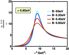
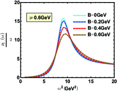
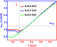
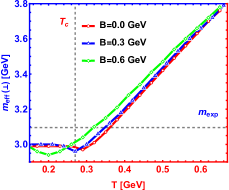
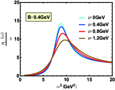
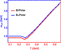
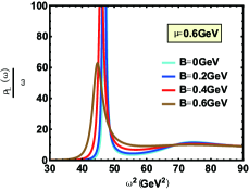
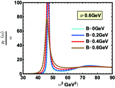
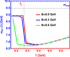
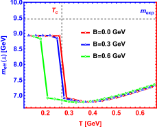
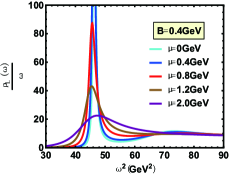
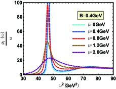
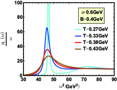
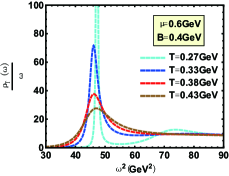
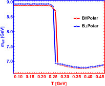
In Fig.1, the spectral function of the state for different magnetic fields parallel and perpendicular to the polarization are shown. The bell shape represents the resonance state and peak position is related to the resonant mass. The width corresponding to half the peak height is the resonant decay width. One can find that increasing magnetic field reduces the height of the peak and enlarges its width of that. This phenomenon indicates that the appearance of magnetic field speeds the dissociation which is consistent with Ref.Braga and Ferreira (2018) where the authors use an Einstein-Maxwell theory. In addition, an interesting phenomenon about effective mass is shown in Fig.2. When magnetic field is parallel to the polarization, the magnetic field reduces the effective mass, reminiscent of the inverse magnetic catalysis at lower temperature, while that is from inverse magnetic catalysis to magnetic catalysis in ref.Braga and Ferreira (2019) where the authors use an Einstein-Maxwell theory. It is worth noting that, after phase transition temperature, our results show the effective mass is almost independent of magnetic field with only slight suppresion, however, the magnetic field presents a magnetic catalysis effect in ref.Braga and Ferreira (2019). When magnetic field is perpendicular to the polarization, our conclusions give that the magnetic field effect on the effective mass is from magnetic catalysis to inverse magnetic catalysis at lower temperature and behaves as magnetic catalysis after phase transition temperature, however, an inverse magnetic catalysis effect is obtained for all temperature in Ref.Braga and Ferreira (2019). Here, we need to point out that in this paper, the effective mass is determined by the energy corresponding to the position of the spectral function peak, while in Ref.Braga and Ferreira (2019), it is determined by the real part of the quasinormal modes.
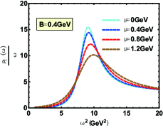
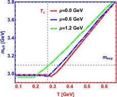
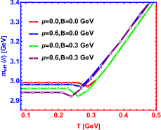
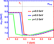
We present the spectral function of the state for different chemical potentials in Fig.3. It can be found that chemical potential has a similar effect as the magnetic field. Increasing chemical potential reduces the height of the peak and increases the width which is consistent with Ref.Braga et al. (2017) where the authors use a generalized soft-wall model. However, attention must be paid to the influence of chemical potential on the peak position, which is plotted in the left picture of Fig.4. The result suggests that the chemical potential gives a suppression effect at lower temperature and presents a enhancement effect at higher temperature on the effective mass, the same conclusion is obtained in Ref.Braga and Da Mata (2020) where the authors use a generalized soft-wall model. However we find that chemical potential effect is more prominent at higher temperature in this paper, while the results from Ref.Braga and Da Mata (2020) shows that the chemical potential effect mainly acts at lower temperature. Besides, the simultaneous effects of and is depicted in the right picture of Fig.4. The superposition of chemical potential and magnetic field effects causes non-trivial behaviors of the effective mass : At lower temperature, there appears constructive interplay on the effective mass between the effects of chemical potential and magnetic field , while at higher temperature, the chemical potential and magnetic field lead to destructive interplay on the effective mass.
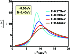
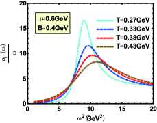
In Fig.5, the behavior of spectral function is extraordinarily sensitive to the temperature of the current physical system. With the increase of the medium temperature, the height of the peak decreases rapidly which is in line with Ref.Braga et al. (2016). The effect of temperature on the width and the position of the peak (see Fig.2 and 4) is similar to that of chemical potential, which is consistent with Ref.Martin Contreras et al. (2021) and the lattice results in Ref.Ding et al. (2019).
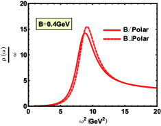
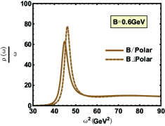
Besides, in Fig.6, we compare the magnetic field parallel to polarization with perpendicular to that. The comparison shows that the melting effect produced by the magnetic field is stronger and the effective mass is smaller in the parallel direction than that in the perpendicular direction, which is diametrically opposite to that found in Ref.Braga and Ferreira (2018) in the EM model. Our result agrees qualitatively with the lattice result of string tension in Ref. Bonati et al. (2016), where it is found that the transverse magnetic field increases the string tension , while the longitudinal magnetic field suppresses the string tension. This difference comes from two aspects: One is this result can be well explained by comparing Eq.(41) and Eq.(42) in terms of appearance, the appearance of the magnetic field in the denominator of the first term on the right of Eq. (41) and the numerator inside the bracket both decrease the value of numerically. In contrast, Eq.(42) does not have a magnetic field, formally. The second is the dilaton introduced in the action, in other words, that is the difference between the EM model and the EMD model. In this paper, we consider the EMD model. The advantages of EMD model can be found in Ref. Zhou et al. (2020). The dilaton will deform the space and influence the magnetic field in different directions. Further, we find EMD model can realize the linear part of Cornell potential extracted from lattice simulation and show the magnetic field in a parallel direction has a large influence on potential. The EM action without the dilaton field cannot get a proper free energy behavior of single quark. The result from lattice Bonati et al. (2016) also favors the EMD model with a dilaton than the EM model.
IV.2 The Result For
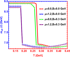
The spectral function for the state with various cases are shown in Fig. 7-Fig. 12. Compared with in this paper and in Ref.Braga and Ferreira (2019), one can find the only difference is from the influence of magnetic field on the peak position of spectral function (effective mass). Whether the magnetic field is perpendicular to or parallel to polarization, Fig.8 reports an inverse magnetic catalysis Thakur and Hirono (2021); Morita and Lee (2010) at lower temperature and a magnetic catalysis Ding et al. (2019); Rothkopf (2017) at higher temperature, which is in line with Ref.Braga and Ferreira (2019). The only difference is that the effective mass mutates at for zero magnetic field and the mutation occurs in a smaller temperature with the increasing magnetic field in our model. The reason for this mutation is that the confinement-deconfinement phase transition here is a first-order phase transition. However, the change of effective mass with temperature is smooth from Ref.Braga and Ferreira (2019), which is because the transition from hadron phase to quark phase is crossover.
For both and , the superposition of chemical potential and magnetic field effects causes non-trivial behaviors of the effective mass : At lower temperature, there appears constructive interplay on the effective mass between the effects of chemical potential and magnetic field , while at higher temperature, the chemical potential and magnetic field lead to destructive interplay on the effective mass. Due to the superposition of two distinct effects between chemical potential and magnetic field, some non-trivial non monotonic behaviors of effective mass appears in the middle temperature region. Of course, the inflection point of this non-trivial behavior strictly depends on the strength of chemical potential, temperature, magnetic field and the interaction between quarkonium. We explain this non-trivial behavior by the interplay of the interaction between the two heavy quarks and the interaction between the medium with each of the heavy quarks. Finally, combined with the behavior of spectral function and the influence of superposition effect of and on effective mass, a general conclusion is obtained, in the strong coupling system, the effective mass is dominated by the depression effect at a lower temperature, smaller chemical potential, weaker magnetic field and shorter distance of interaction; however, the effective mass is dominated by the enhancement effect at a higher temperature, higher chemical potential, stronger magnetic field and longer distance of the heavy quarks. In other words, the effective mass is closely related to the coupling strength and the distance of interaction between the pair.
V acknowledgments
This work is supported by the National Natural Science Foundation of China by Grant Nos. 11735007,11890711, and 11890710. In addition, the first author wants to thank Hai-cang Ren and Zhou-Run Zhu for helpful discussions.
Reference
References
- Gyulassy and McLerran (2005) M. Gyulassy and L. McLerran, Nucl. Phys. A 750, 30 (2005), eprint nucl-th/0405013.
- Maldacena (1998) J. M. Maldacena, Adv. Theor. Math. Phys. 2, 231 (1998), eprint hep-th/9711200.
- Witten (1998) E. Witten, Adv. Theor. Math. Phys. 2, 253 (1998), eprint hep-th/9802150.
- de Haro et al. (2001) S. de Haro, S. N. Solodukhin, and K. Skenderis, Commun. Math. Phys. 217, 595 (2001), eprint hep-th/0002230.
- Rey and Yee (2001) S.-J. Rey and J.-T. Yee, Eur. Phys. J. C 22, 379 (2001), eprint hep-th/9803001.
- Klebanov and Witten (1999) I. R. Klebanov and E. Witten, Nucl. Phys. B 556, 89 (1999), eprint hep-th/9905104.
- Karch and Katz (2002) A. Karch and E. Katz, JHEP 06, 043 (2002), eprint hep-th/0205236.
- Erlich et al. (2005) J. Erlich, E. Katz, D. T. Son, and M. A. Stephanov, Phys. Rev. Lett. 95, 261602 (2005), eprint hep-ph/0501128.
- Freedman et al. (1999) D. Z. Freedman, S. D. Mathur, A. Matusis, and L. Rastelli, Nucl. Phys. B 546, 96 (1999), eprint hep-th/9804058.
- Policastro et al. (2002) G. Policastro, D. T. Son, and A. O. Starinets, JHEP 09, 043 (2002), eprint hep-th/0205052.
- Casalderrey-Solana et al. (2014) J. Casalderrey-Solana, H. Liu, D. Mateos, K. Rajagopal, and U. A. Wiedemann, Gauge/String Duality, Hot QCD and Heavy Ion Collisions (Cambridge University Press, 2014), ISBN 978-1-139-13674-7, eprint 1101.0618.
- Gopakumar and Vafa (1999) R. Gopakumar and C. Vafa, Adv. Theor. Math. Phys. 3, 1415 (1999), eprint hep-th/9811131.
- Emparan et al. (1999) R. Emparan, C. V. Johnson, and R. C. Myers, Phys. Rev. D 60, 104001 (1999), eprint hep-th/9903238.
- Caldarelli et al. (2000) M. M. Caldarelli, G. Cognola, and D. Klemm, Class. Quant. Grav. 17, 399 (2000), eprint hep-th/9908022.
- Hawking et al. (1999) S. W. Hawking, C. J. Hunter, and M. Taylor, Phys. Rev. D 59, 064005 (1999), eprint hep-th/9811056.
- Matsui and Satz (1986) T. Matsui and H. Satz, Phys. Lett. B 178, 416 (1986).
- Hatsuda and Kunihiro (1985) T. Hatsuda and T. Kunihiro, Phys. Rev. Lett. 55, 158 (1985).
- Asakawa and Hatsuda (2004) M. Asakawa and T. Hatsuda, Phys. Rev. Lett. 92, 012001 (2004), eprint hep-lat/0308034.
- Datta et al. (2004) S. Datta, F. Karsch, P. Petreczky, and I. Wetzorke, Phys. Rev. D 69, 094507 (2004), eprint hep-lat/0312037.
- Skokov et al. (2009) V. Skokov, A. Y. Illarionov, and V. Toneev, Int. J. Mod. Phys. A 24, 5925 (2009), eprint 0907.1396.
- Bzdak and Skokov (2012) A. Bzdak and V. Skokov, Phys. Lett. B 710, 171 (2012), eprint 1111.1949.
- Zhu et al. (2020) Z.-R. Zhu, D.-f. Hou, and X. Chen, Eur. Phys. J. C 80, 550 (2020), eprint 1912.05806.
- Zhu et al. (2021) Z.-R. Zhu, Y.-K. Liu, and D. Hou (2021), eprint 2108.05148.
- Voronyuk et al. (2011) V. Voronyuk, V. D. Toneev, W. Cassing, E. L. Bratkovskaya, V. P. Konchakovski, and S. A. Voloshin, Phys. Rev. C 83, 054911 (2011), eprint 1103.4239.
- Roy et al. (2017) V. Roy, S. Pu, L. Rezzolla, and D. H. Rischke, Phys. Rev. C 96, 054909 (2017), eprint 1706.05326.
- Tuchin (2013) K. Tuchin, Adv. High Energy Phys. 2013, 490495 (2013), eprint 1301.0099.
- Seiberg (1995) N. Seiberg, Nucl. Phys. B 435, 129 (1995), eprint hep-th/9411149.
- Gusynin et al. (1996) V. P. Gusynin, V. A. Miransky, and I. A. Shovkovy, Nucl. Phys. B 462, 249 (1996), eprint hep-ph/9509320.
- Kharzeev and Yee (2011) D. E. Kharzeev and H.-U. Yee, Phys. Rev. D 83, 085007 (2011), eprint 1012.6026.
- Cao et al. (2020) X. Cao, H. Liu, and D. Li, Phys. Rev. D 102, 126014 (2020), eprint 2009.00289.
- Preis et al. (2011) F. Preis, A. Rebhan, and A. Schmitt, JHEP 03, 033 (2011), eprint 1012.4785.
- Albash et al. (2008) T. Albash, V. G. Filev, C. V. Johnson, and A. Kundu, JHEP 07, 080 (2008), eprint 0709.1547.
- Kalaydzhyan and Kirsch (2011) T. Kalaydzhyan and I. Kirsch, Phys. Rev. Lett. 106, 211601 (2011), eprint 1102.4334.
- Cao et al. (2021) X. Cao, S. Qiu, H. Liu, and D. Li, JHEP 08, 005 (2021), eprint 2102.10946.
- Finazzo et al. (2016) S. I. Finazzo, R. Critelli, R. Rougemont, and J. Noronha, Phys. Rev. D 94, 054020 (2016), [Erratum: Phys.Rev.D 96, 019903 (2017)], eprint 1605.06061.
- Preis et al. (2013) F. Preis, A. Rebhan, and A. Schmitt, Lect. Notes Phys. 871, 51 (2013), eprint 1208.0536.
- Rougemont et al. (2016) R. Rougemont, R. Critelli, and J. Noronha, Phys. Rev. D 93, 045013 (2016), eprint 1505.07894.
- Bu et al. (2013) Y.-Y. Bu, J. Erdmenger, J. P. Shock, and M. Strydom, JHEP 03, 165 (2013), eprint 1210.6669.
- Hoyos et al. (2011) C. Hoyos, T. Nishioka, and A. O’Bannon, JHEP 10, 084 (2011), eprint 1106.4030.
- Gorsky et al. (2011) A. Gorsky, P. N. Kopnin, and A. V. Zayakin, Phys. Rev. D 83, 014023 (2011), eprint 1003.2293.
- Cai et al. (2013) R.-G. Cai, S. He, L. Li, and L.-F. Li, JHEP 12, 036 (2013), eprint 1309.2098.
- Mamo (2015) K. A. Mamo, JHEP 05, 121 (2015), eprint 1501.03262.
- Jensen et al. (2010) K. Jensen, A. Karch, and E. G. Thompson, JHEP 05, 015 (2010), eprint 1002.2447.
- Dudal et al. (2016) D. Dudal, D. R. Granado, and T. G. Mertens, Phys. Rev. D 93, 125004 (2016), eprint 1511.04042.
- Jokela et al. (2012) N. Jokela, G. Lifschytz, and M. Lippert, JHEP 05, 105 (2012), eprint 1204.3914.
- Callebaut et al. (2013) N. Callebaut, D. Dudal, and H. Verschelde, JHEP 03, 033 (2013), eprint 1105.2217.
- Filev and Raskov (2010) V. G. Filev and R. C. Raskov, Adv. High Energy Phys. 2010, 473206 (2010), eprint 1010.0444.
- Gürsoy et al. (2017) U. Gürsoy, I. Iatrakis, M. Järvinen, and G. Nijs, JHEP 03, 053 (2017), eprint 1611.06339.
- Evans et al. (2016) N. Evans, C. Miller, and M. Scott, Phys. Rev. D 94, 074034 (2016), eprint 1604.06307.
- Braga and Ferreira (2018) N. R. F. Braga and L. F. Ferreira, Phys. Lett. B 783, 186 (2018), eprint 1802.02084.
- Colangelo et al. (2013) P. Colangelo, F. Giannuzzi, S. Nicotri, and F. Zuo, Phys. Rev. D 88, 115011 (2013), eprint 1308.0489.
- Gursoy et al. (2018) U. Gursoy, M. Jarvinen, and G. Nijs, Phys. Rev. Lett. 120, 242002 (2018), eprint 1707.00872.
- Braga and Ferreira (2019) N. R. F. Braga and L. F. Ferreira, Phys. Lett. B 795, 462 (2019), eprint 1905.11309.
- Zhu et al. (2019) Z.-R. Zhu, S.-Q. Feng, Y.-F. Shi, and Y. Zhong, Phys. Rev. D 99, 126001 (2019), eprint 1901.09304.
- Li et al. (2017) D. Li, M. Huang, Y. Yang, and P.-H. Yuan, JHEP 02, 030 (2017), eprint 1610.04618.
- Zhou et al. (2020) J. Zhou, X. Chen, Y.-Q. Zhao, and J. Ping, Phys. Rev. D 102, 086020 (2020), eprint 2006.09062.
- Feng et al. (2020) S.-Q. Feng, Y.-Q. Zhao, and X. Chen, Phys. Rev. D 101, 026023 (2020), eprint 1910.05668.
- Fujita et al. (2009) M. Fujita, K. Fukushima, T. Misumi, and M. Murata, Phys. Rev. D 80, 035001 (2009), eprint 0903.2316.
- Umeda et al. (2001) T. Umeda, R. Katayama, O. Miyamura, and H. Matsufuru, Int. J. Mod. Phys. A 16, 2215 (2001), eprint hep-lat/0011085.
- Ghoroku et al. (2006) K. Ghoroku, N. Maru, M. Tachibana, and M. Yahiro, Phys. Lett. B 633, 602 (2006), eprint hep-ph/0510334.
- Ávila and Patiño (2020) D. Ávila and L. Patiño, JHEP 06, 010 (2020), eprint 2002.02470.
- Braga et al. (2017) N. R. F. Braga, L. F. Ferreira, and A. Vega, Phys. Lett. B 774, 476 (2017), eprint 1709.05326.
- Hou and Ren (2008) D. Hou and H.-c. Ren, JHEP 01, 029 (2008), eprint 0710.2639.
- Bohra et al. (2020) H. Bohra, D. Dudal, A. Hajilou, and S. Mahapatra, Phys. Lett. B 801, 135184 (2020), eprint 1907.01852.
- Dudal and Mahapatra (2017) D. Dudal and S. Mahapatra, Phys. Rev. D 96, 126010 (2017), eprint 1708.06995.
- Iqbal and Liu (2009) N. Iqbal and H. Liu, Phys. Rev. D 79, 025023 (2009), eprint 0809.3808.
- Tanabashi et al. (2018) M. Tanabashi et al. (Particle Data Group), Phys. Rev. D 98, 030001 (2018).
- Son and Starinets (2002) D. T. Son and A. O. Starinets, JHEP 09, 042 (2002), eprint hep-th/0205051.
- Karch et al. (2006) A. Karch, E. Katz, D. T. Son, and M. A. Stephanov, Phys. Rev. D 74, 015005 (2006), eprint hep-ph/0602229.
- Martin Contreras et al. (2021) M. A. Martin Contreras, S. Diles, and A. Vega, Phys. Rev. D 103, 086008 (2021), eprint 2101.06212.
- Braga and Da Mata (2020) N. R. F. Braga and R. Da Mata, Phys. Lett. B 804, 135381 (2020), eprint 1910.13498.
- Braga et al. (2016) N. R. F. Braga, M. A. Martin Contreras, and S. Diles, Eur. Phys. J. C 76, 598 (2016), eprint 1604.08296.
- Ding et al. (2019) H.-T. Ding, O. Kaczmarek, A.-L. Kruse, R. Larsen, L. Mazur, S. Mukherjee, H. Ohno, H. Sandmeyer, and H.-T. Shu, Nucl. Phys. A 982, 715 (2019), eprint 1807.06315.
- Bonati et al. (2016) C. Bonati, M. D’Elia, M. Mariti, M. Mesiti, F. Negro, A. Rucci, and F. Sanfilippo, Phys. Rev. D 94, 094007 (2016), eprint 1607.08160.
- Thakur and Hirono (2021) L. Thakur and Y. Hirono (2021), eprint 2111.08225.
- Morita and Lee (2010) K. Morita and S. H. Lee, Phys. Rev. D 82, 054008 (2010), eprint 0908.2856.
- Rothkopf (2017) A. Rothkopf, EPJ Web Conf. 137, 07018 (2017), eprint 1611.06518.