Albert Lin \Emailalbert.k.lin@usc.edu
\NameSomil Bansal \Emailsomilban@usc.edu
\addrDepartment of Electrical and Computer Engineering, University of Southern California, CA, USA
Verification of Neural Reachable Tubes via Scenario Optimization and Conformal Prediction
Abstract
Learning-based approaches for controlling safety-critical autonomous systems are rapidly growing in popularity; thus, it is important to provide rigorous and robust assurances on their performance and safety. Hamilton-Jacobi (HJ) reachability analysis is a popular formal verification tool for providing such guarantees, since it can handle general nonlinear system dynamics, bounded adversarial system disturbances, and state and input constraints. However, it involves solving a Partial Differential Equation (PDE), whose computational and memory complexity scales exponentially with respect to the state dimension, making its direct use on large-scale systems intractable. To overcome this challenge, neural approaches, such as DeepReach, have been used to synthesize reachable tubes and safety controllers for high-dimensional systems. However, verifying these neural reachable tubes remains challenging. In this work, we propose two different verification methods, based on robust scenario optimization and conformal prediction, to provide probabilistic safety guarantees for neural reachable tubes. Our methods allow a direct trade-off between resilience to outlier errors in the neural tube, which are inevitable in a learning-based approach, and the strength of the probabilistic safety guarantee. Furthermore, we show that split conformal prediction, a widely used method in the machine learning community for uncertainty quantification, reduces to a scenario-based approach, making the two methods equivalent not only for verification of neural reachable tubes but also more generally. To our knowledge, our proof is the first in the literature to show a strong relationship between the highly related but disparate fields of conformal prediction and scenario optimization. Finally, we propose an outlier-adjusted verification approach that harnesses information about the error distribution in neural reachable tubes to recover greater safe volumes. We demonstrate the efficacy of the proposed approaches for the high-dimensional problems of multi-vehicle collision avoidance and rocket landing with no-go zones.
keywords:
Probabilistic Safety Guarantees, Safety-Critical Learning, Neural Certificates, Hamilton-Jacobi Reachability Analysis, Scenario Optimization, Conformal Prediction1 Introduction
It is important to design provably safe controllers for autonomous systems. Hamilton-Jacobi (HJ) reachability analysis provides a powerful framework to design such controllers for general nonlinear dynamical systems (Lygeros, 2004; Mitchell et al., 2005). In reachability analysis, safety is characterized by the system’s Backward Reachable Tube (BRT). This is the set of states from which trajectories will eventually reach a given target set despite the best control effort. Thus, if the target set represents undesirable states, the BRT represents unsafe states and should be avoided. Along with the BRT, reachability analysis provides a safety controller to keep the system outside the BRT.
Traditionally, the BRT computation in HJ reachability is formulated as an optimal control problem. The BRT can then be obtained as a sub-zero level solution of the corresponding value function. Obtaining the value function requires solving a partial differential equation (PDE) over a state-space grid, resulting in an exponentially scaling computation complexity with the number of states (Bansal et al., 2017). To overcome this challenge, a variety of solutions have been proposed that trade off between the class of dynamics they can handle, the approximation quality of the BRT, and the required computation. These include specialized methods for linear and affine dynamics (Greenstreet and Mitchell, 1998; Frehse et al., 2011; Kurzhanski and Varaiya, 2000, 2002; Maidens et al., 2013; Girard, 2005; Althoff et al., 2010; Bak et al., 2019; Nilsson and Ozay, 2016), polynomial dynamics (Majumdar et al., 2014; Majumdar and Tedrake, 2017; Dreossi et al., 2016; Henrion and Korda, 2014), monotonic dynamics (Coogan and Arcak, 2015), and convex dynamics (Chow et al., 2017) (see Bansal et al. (2017); Bansal and Tomlin (2021) for a survey).
Owing to the success of deep learning, there has also been a surge of interest in approximating high-dimensional BRTs (Rubies-Royo et al., 2019; Fisac et al., 2019; Djeridane and Lygeros, 2006; Niarchos and Lygeros, 2006; Darbon et al., 2020) and optimal controllers (Onken et al., 2022) through deep neural networks (DNNs). Building upon this line of work, Bansal and Tomlin (2021) have proposed DeepReach – a toolbox that leverages recent advances in neural implicit representations and neural PDE solvers to compute a value function and a safety controller for high-dimensional systems. Compared to the aforementioned methods, DeepReach can handle general nonlinear dynamics, the presence of exogenous disturbances, as well as state and input constraints during the BRT computation. Consequently, methods for verifying neural reachable tubes have been proposed. For example, Lin and Bansal (2023) propose an iterative scenario-based method (Campi et al., 2009) to recover probabilistically safe reachable tubes from DeepReach solutions up to a desired confidence level and bound on violation rate. Unfortunately, the method does not allow an after-the-fact risk-return trade-off, and as a result, it is highly sensitive to outlier errors in the learned solutions. This can lead to highly conservative reachable tubes and a severe loss of recovery in the case of stringent safety requirements, as we demonstrate in our case studies.
In this work, we propose two different verification methods, one based on robust scenario optimization and the other based on conformal prediction, to provide probabilistic safety guarantees for neural reachable tubes. Both methods are resilient to the outlier errors in neural reachable tubes and automatically trade-off the strength of the probabilistic safety guarantees based on the outlier rate. The proposed methods can evaluate any candidate tube and are not restricted to a specific class of system dynamics or value functions. We further prove that these seemingly different verification methods naturally reduce to one another, providing a unifying viewpoint for uncertainty quantification (typical use case of conformal prediction) and error optimization (typical use case of scenario optimization) in neural reachable tubes. Based on these insights, we propose an outlier-adjusted verification approach that can recover a greater safe volume from a neural reachable tube by harnessing information about the distribution of error in the learned solution. To summarize, the key contributions of this paper are:
-
•
probabilistic safety verification methods for neural reachable tubes that enable a direct trade-off between resilience and the probabilistic strength of safety,
-
•
a proof that split conformal prediction reduces to a scenario-based approach in general, demonstrating a strong relationship between the two highly related but disparate fields,
-
•
an outlier-adjusted verification approach that recovers greater safe volumes from tubes, and
-
•
a demonstration of the proposed approaches for the high-dimensional problems of multi-vehicle collision avoidance and rocket landing with no-go zones.
2 Problem Setup
Consider a dynamical system with state , control , and dynamics governing how evolves over time until a final time . Let denote the state achieved at time by starting at initial state and time and applying control over . Let represent a target set that the agent wants to either reach (e.g. goal states) or avoid (e.g. obstacles).
Running example: Multi-Vehicle Collision Avoidance. Consider a 9D multi-vehicle collision avoidance system with 3 independent Dubins3D cars: . has position , heading , constant velocity , and steering control . The dynamics of are: . is the set of states where any of the vehicle pairs is in collision: , where is the distance between and . We set: .
In this setting, we are interested in computing the system’s initial-time Backward Reachable Tube, which we denote as BRT. We define BRT as the set of all initial states in from which the agent will eventually reach within the time horizon , despite best control efforts: . When represents unsafe states for the system, as it does in our running example, staying outside of BRT is desirable. When instead represents the states that the agent wants to reach, BRT is defined as the set of all initial states in from which the agent, acting optimally, can eventually reach within . Thus, staying within BRT is desirable.
The above 9D system is intractable for traditional grid-based methods, motivating the use of DeepReach to learn a neural BRT. Our goal in this work is to recover an approximation of the safe set with probabilistic guarantees. Specifically, we want to find such that for some violation parameter . When represents goal states, we want .
3 Background: Hamilton-Jacobi Reachability, DeepReach, and Safety Verification
Here, we provide a quick overview of Hamilton-Jacobi reachability analysis, a specific toolbox, DeepReach, to compute high-dimensional neural reachable tubes, and an iterative scenario-based method for recovering probabilistically safe tubes from learning-based methods like DeepReach.
3.1 Hamilton-Jacobi (HJ) Reachability
In HJ reachability, computing BRT is formulated as an optimal control problem. We will explain it in the context of being a set of undesirable states. In the end, we will comment on when is a set of desirable states and refer interested readers to Bansal et al. (2017) for other cases.
We first define a target function such that the sub-zero level of yields : . is commonly a signed distance function to . For example, we can choose for our running example in \sectionrefsec:problem_setup. Next, we define the cost function of a state corresponding to some policy to be the minimum of over its trajectory: . Since the system wants to avoid , our goal is to maximize . Thus, the value function corresponding to this optimal control problem is:
| (1) |
By defining our optimal control problem in this way, we can recover BRT using the value function. In particular, the value function being sub-zero implies that the target function is sub-zero somewhere along the optimal trajectory, or in other words, that the system has reached . Thus, BRT is given as the sub-zero level set of the value function at the initial time: . The value function in Equation (1) can be computed using dynamic programming, resulting in the following final value Hamilton-Jacobi-Bellman Variational Inequality (HJB-VI): , with the terminal value function . and represent the time and spatial gradients of . is the Hamiltonian that encodes the role of dynamics and the optimal control: . The value function in Equation (1) induces the optimal safety controller: . Intuitively, the safety controller aligns the system dynamics in the direction of the value function’s gradient, thus steering the system towards higher-value states, i.e., away from .
We have just explained the case where represents a set of undesirable states. When the system instead wants to reach , an infimum is used instead of a supremum in Equation . The control wants to reach , hence there is a minimum instead of a maximum in the Hamiltonian and optimal safety controller equations. See Bansal et al. (2017) for details on other reachability cases.
Traditionally, the value function is computed by solving the HJB-VI over a discretized grid in the state space. Unfortunately, doing so involves computation whose memory and time complexity scales exponentially with respect to the system dimension, making these methods practically intractable for high-dimensional systems, such as those beyond 5D. Fortunately, a deep learning approach, DeepReach, has been proposed to enable HJ reachability for high-dimensional systems.
3.2 DeepReach and an Iterative Scenario-Based Probabilistic Safety Verification Method
Instead of solving the HJB-VI over a grid, DeepReach (Bansal and Tomlin, 2021) learns a parameterized approximation of the value function using a sinusoidal deep neural network (DNN). Thus, memory and complexity requirements for training scale with the value function complexity rather than the grid resolution, allowing it to obtain BRTs for high-dimensional systems. DeepReach trains the DNN via self-supervision on the HJB-VI itself. Ultimately, it takes as input a state and time , and it outputs a learned value function . also induces a corresponding safe policy , as well as a BRT (referred to as the neural reachable tube from hereon).
However, the neural reachable tube will only be as accurate as . To obtain a provably safe BRT, Lin and Bansal (2023) propose a uniform value correction bound which is defined, for the avoid case, as the maximum learned value of an unsafe state under the induced policy: . The authors show that the super- level set of is provably safe under the policy . They also propose an iterative scenario-based probabilistic verification method for computing an approximation of from finite random samples that satisfies a desired confidence level and violation rate. However, the method is sensitive to outlier errors in the neural reachable tube and can result in very conservative safe sets. Specifically, it does not provide safety assurances for safe sets with nonzero empirical safety violations.
In this work, we propose probabilistic safety verification methods that allow nonzero empirical safety violations at the cost of the probabilistic strength of safety. This enables a direct trade-off between resilience to outlier errors and the strength of the safety guarantee.
Remark 3.1.
Although we work with DeepReach solutions in particular for our problem setup, our proposed approaches can verify any general and , regardless of whether DeepReach, a numerical PDE solver, or some other tool is used to obtain them.
4 Robust Scenario-Based Probabilistic Safety Verification Method
Here, we propose a robust scenario-based probabilistic safety verification method for neural reachable tubes. The new method is a straightforward application of a scenario-based sampling-and-discarding approach to chance-constrained optimization problems, which quantifies the trade-off between feasibility and performance of the optimal solution based on finite samples (Campi and Garatti, 2011). First, we explain the method when represents undesirable states. In the end, we comment on when represents desirable states.
Procedures: Let be a neural safe set that is, in the avoid case, the complement of the neural reachable tube being verified. In our case, is typically a super- level set of the learned value function . Ideally, any super- level set of for should be a valid safe set; however, due to learning errors, that might not be true in practice. To provide a probabilistic safety assurance for , we first sample independent and identically distributed (i.i.d.) states from according to some probability distribution over . Since is defined implicitly by , we use rejection sampling. We next compute the costs for by rolling out the system trajectory from under . Let refer to the number of “outliers” - samples that are empirically unsafe, i.e., . Then the following theorem provides a probabilistic guarantee on the safety of the neural reachable tube and its complement, the neural safe set :
Theorem 4.1 (Robust Scenario-Based Probabilistic Safety Verification).
Select a safety violation parameter and a confidence parameter such that
| (2) |
where and are as defined above. Then, with probability at least , the following holds:
| (3) |
All proofs can be found in the Appendix of the extended version of this article111See \urlhttps://sia-lab-git.github.io/Verification_of_Neural_Reachable_Tubes.pdf. Disregarding the confidence parameter for a moment, \theoremreftheorem:scenario-based_method states that the fraction of that is unsafe is bounded above by the violation parameter , where is computed empirically using Equation (2) based on the outlier rate encountered within samples. is thus a reflection of the safety quality of , which degrades with the increase in the number of outliers , as expected. This can also be seen for the running example in \figurereffig:fixed_N (the red curve). Overall, \theoremreftheorem:scenario-based_method allows us to compute probabilistic safety guarantees for any neural set based on a finite number of samples. Subsequently, this result can be used to find some for which is smaller than a desired threshold, as we discuss later in this section.
To interpret , note that is a random variable that depends on the randomly sampled . It may be the case that we just happen to draw an unrepresentative sample, in which case the bound does not hold. controls the probability of this adverse event happening, which regards the correctness of the probabilistic safety guarantee in Equation (3). Fortunately, goes to exponentially with , so can be chosen to be an extremely small value, such as , when we sample large . will then be so close to that it does not have any practical importance.
We have just explained the robust scenario-based probabilistic safety verification method in the case where represents undesirable states. When the system instead wants to reach , will be a sublevel set instead of a superlevel set of the learned value function. The cost inequality should be flipped when computing , and the value inequality should be flipped in Equation (3).
4.1 Comparison of Robust and Iterative Scenario-Based Probabilistic Safety Verification
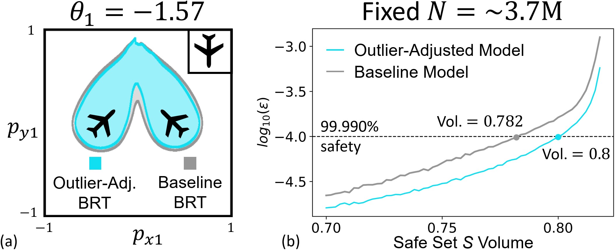
The key difference between the proposed robust scenario-based method and the iterative scenario-based method discussed in \sectionrefsec:deepreach_iterative_verification is that the former can handle nonzero empirical safety violations . This enables several crucial advantages that we demonstrate in \figurereffig:fixed_N,fig:diff_N for a solution learned by DeepReach on the multi-vehicle collision avoidance running example in \sectionrefsec:problem_setup. We have fixed the confidence parameter to be so close to that it has no practical significance ( plays the same role in both methods).
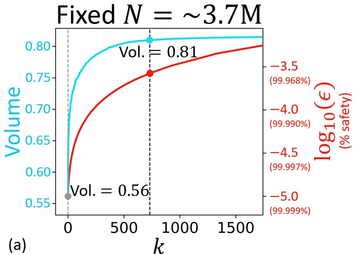
Firstly, for a fixed simulation budget , the robust method allows one to trade off the probabilistic strength of safety (increasing ) for resilience (increasing ). In other words, the method can verify any given neural safe set in an outlier-robust fashion by automatically attenuating the level of safety assurance based on the number of empirical outliers (i.e., safety violations). The iterative method, in contrast, can only verify a region that is outlier-free. Consequently, the robust method enables one to engage in a trade-off if a large increase in safe set volume can be attained by a tolerable decrease in safety, as illustrated in \figurereffig:fixed_N.
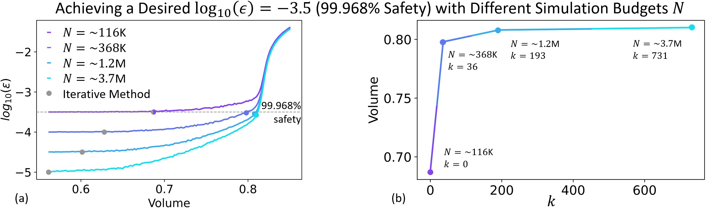
Secondly, by allowing nonzero safety violations , the robust method provides stronger safety assurances for a fixed volume with increment in the simulation budget , as long as the outlier rate does not grow substantially with . Thus, with more simulation effort, significantly larger volumes can be attained for a desired safety strength as shown in \figurereffig:diff_N. Incrementing in the iterative method, on the other hand, will only correspond to verifying smaller volumes at a stronger . It cannot verify larger volumes for a fixed , because empirical safety violations will be introduced. \figurereffig:diff_N shows how the robust method (curves) adds a new degree of freedom for computing safety assurances compared to the iterative method (grey points).
5 Conformal Probabilistic Safety Verification Method
We now propose a conformal probabilistic safety verification method for neural reachable tubes which is intended to be the direct analogue of the robust scenario-based method in \sectionrefsec:scenario-based_method. The method is a straightforward application of split conformal prediction, a widely used method in the machine learning community for uncertainty quantification (Angelopoulos and Bates, 2023).
Using the same procedures as described in \sectionrefsec:scenario-based_method, split conformal prediction can be used instead of robust scenario optimization to provide a probabilistic guarantee on the safety of the neural reachable tube and its complement, the neural safe set :
Theorem 5.1 (Conformal Probabilistic Safety Verification).
Let the number of outliers and the number of samples be as defined in the procedures in \sectionrefsec:scenario-based_method, then:
| (4) |
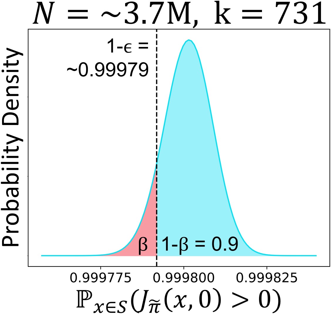
theorem:conformal_method can be established via a straightforward application of conformal prediction with as the scoring function. The proof is in the Appendix of the extended version of this article1. The above theorem states that the fraction of that is safe is distributed according to the Beta distribution with shape parameters and . Intuitively, the mass in the distribution shifts towards as increases for a fixed , implying that it is more likely that a smaller fraction of is safe, as expected. For a fixed ratio , controls how concentrated the mass is around the mean; i.e., for larger sample sizes , we can more confidently determine the fraction of that is safe.
To better understand \theoremreftheorem:conformal_method, we show in \figurereffig:beta the Beta distribution of for a solution learned by DeepReach on the multi-vehicle collision avoidance running example in \sectionrefsec:problem_setup, for which outliers are found from samples.
Remark 5.2.
The mean of the Beta distribution in Equation (4) is given as , which is roughly the fraction of the empirically safe samples. One can immediately derive that the safety probability of , marginalized over the sampled “calibration” states, is given as: , which precisely resembles the most commonly used coverage property of split conformal prediction.
Even though \theoremreftheorem:conformal_method provides the distribution of the safety level, when we compute safety assurances in practice, it is often desirable to know a lower-bound on the safety level with at least some desired confidence. This corresponds to choosing a lower-bound whose accumulated probability mass is smaller than some confidence parameter (shaded red in \figurereffig:beta). The following lemma formalizes this by using the CDF of the Beta distribution in \theoremreftheorem:conformal_method.
Lemma 5.3 (Conformal Probabilistic Safety Verification).
Select a safety violation parameter and a confidence parameter such that
| (5) |
where and are as defined above. Then, with probability at least , the following holds:
| (6) |
lemma:conformal_method is, in fact, precisely the same result as obtained by \theoremreftheorem:scenario-based_method using robust scenario optimization. This is no coincidence, as one can show that split conform prediction more generally reduces to a robust scenario-optimization problem.
Remark 5.4.
In general, a split conformal prediction problem can be reduced to a robust scenario-optimization problem. This is proven in the Appendix of the extended version of this article.1
Due to the equivalence between conformal method and robust scenario-based methods, the analysis in \sectionrefsec:scenario-based_method holds here as well. More generally, we hope that this insight will lead to future research into further investigating the close relationship between the two methods.
6 Outlier-Adjusted Probabilistic Safety Verification Approach
The verification methods in \sectionrefsec:scenario-based_method,sec:conformal_method are limited by the quality of the neural reachable tube. Although they can account for outliers, the computed safety level can be low if the outlier rate is high. This can lead to significant losses in the safe volume, as demonstrated in \sectionrefsec:rocketlanding,sec:reachavoidrocketlanding.
To address this issue, we propose an outlier-adjusted approach that can recover a larger safe volume for any desired . Note that in the verification methods, the key quantity which determines is the number of safety violations . This corresponds to the number of samples which are marked safe by membership in , i.e., , but are not guaranteed to be safe, i.e., . It is easy to see that the best we can do to simultaneously minimize and maximize volume is to compute as the super- level set of the induced cost function . For example, the largest possible that is guaranteed to be violation-free is precisely the super-zero level set of . Thus, our overall approach will be to refine so that it more accurately reflects .
Modeling can be formulated as a supervised learning problem, since we can sample a state and compute its cost in simulation. We learn an approximation by retraining on a training dataset of samples, . Specifically, we use the weighted MSE loss , where if the error is conservative , otherwise . We introduce as a hyperparameter to underweight conservative errors because in the end, we are concerned with recovering larger safe volumes. Thus, selecting a small allows us to focus on reducing optimistic errors which are more safety-critical and correspond to outlier safety violations.
To avoid overfitting, we select the training checkpoint that performs best on a validation dataset . The validation metric we use is the maximum learned cost of an empirically unsafe state: , which one can think of as a proxy for the recoverable safe volume. We demonstrate the efficacy of the proposed outlier-adjusted approach for the high-dimensional systems of multi-vehicle collision avoidance and rocket landing with no-go zones. For all case studies, we set during retraining, fix the confidence parameter and find a safe volume that satisfies ( safety) using the robust method in \sectionrefsec:scenario-based_method.
6.1 Multi-Vehicle Collision Avoidance
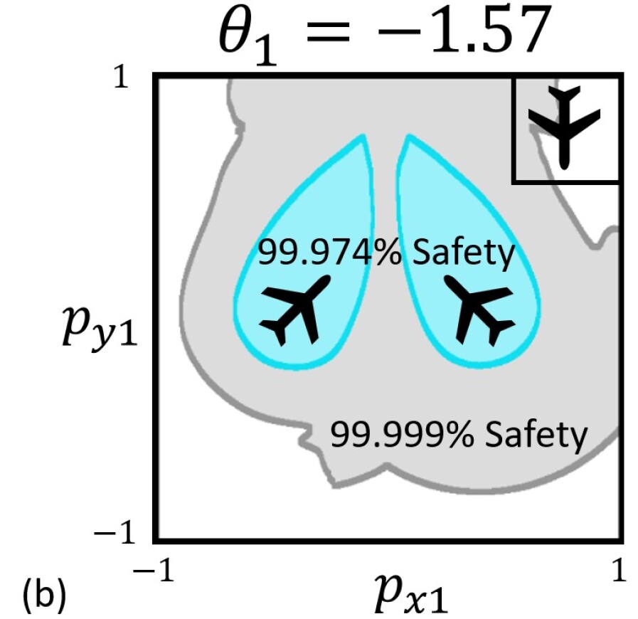
In \figurereffig:multivehicle, we compare our outlier-adjusted approach (blue) to the baseline (grey) for a DeepReach solution trained on the multi-vehicle collision avoidance running example in \sectionrefsec:problem_setup. A increase in the safe volume is attained, shown by the tightened BRT. Note that the largest visual difference in the BRT is where the third vehicle is between the two others; intuitively, the safety in this region is likely more difficult to model by the baseline approach.
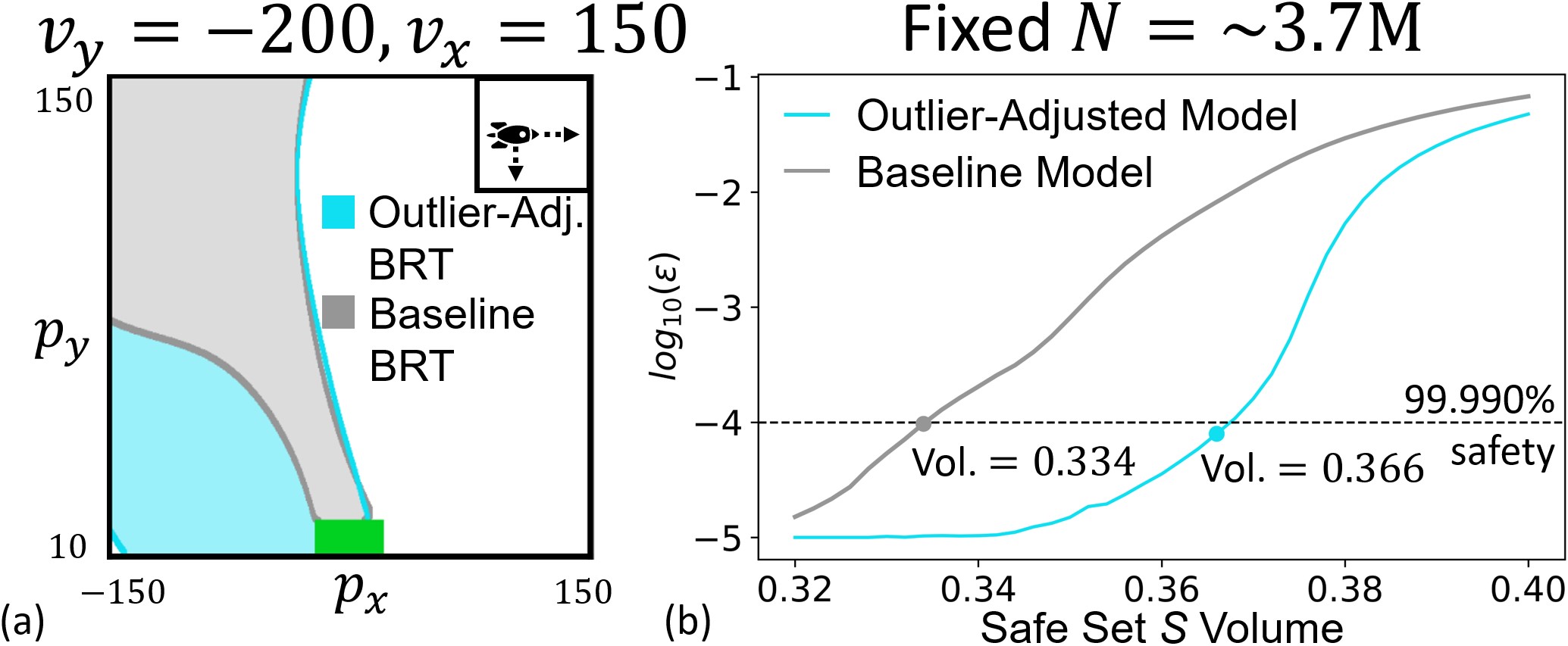
6.2 Rocket Landing
We now apply our approach to a 6D rocket landing system with position , heading , velocity , angular velocity , and torque controls . The dynamics are: , where is acceleration due to gravity. The target set is the set of states where the rocket reaches a rectangular landing zone of side length 20m centered at the origin: . Note that we want to reach , so the BRT now represents the safe set. Results are shown in \figurereffig:rocketlanding. Interestingly, a large increase in the volume of the safe set is recovered using the proposed approach, particularly near the lower-left part of the state space. Further investigation reveals that the trajectories starting from these states exit the training regime south. This highlights a general limitation of computing the value function over a constrained state space where information is propagated via dynamic programming, which affects both learning-based methods and traditional grid-based methods. Nevertheless, in this case, the relative order of the value function levels is still preserved, leading to a high quality safe policy and recovery of a larger safe volume.
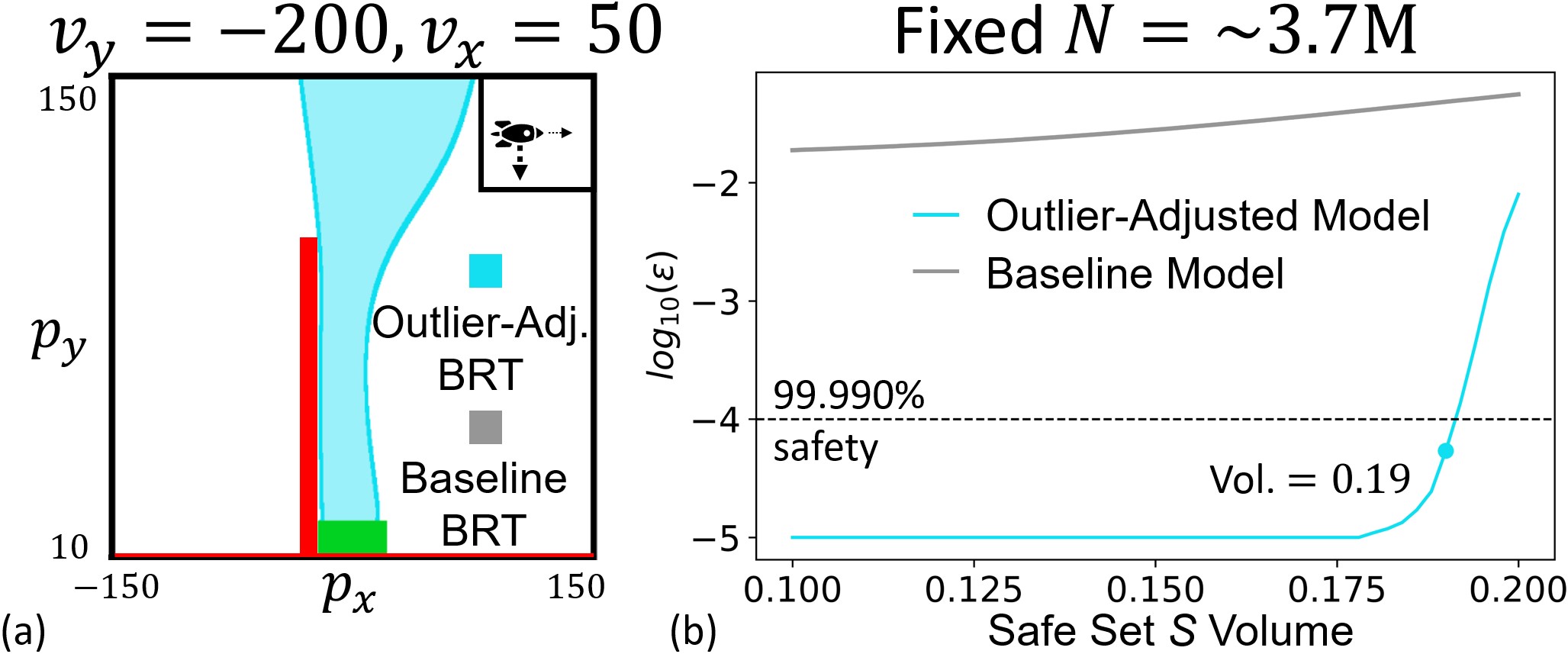
6.3 Rocket Landing with No-Go Zones
We now consider the rocket landing problem in a constrained airspace where we have no-go zones of height 100m and width 10m to the left of the landing zone and where altitude is below the landing zone. Safety in this case takes the form of a reach-avoid set - the rocket needs to reach the landing zone while avoiding the no-go zones. An analogous HJI-VI to the one in \sectionrefsec:background_reachability can be derived for this case, whose solution can be computed using DeepReach. However, since reach-avoid problems are more complex than just the reach or avoid problem, the DeepReach solution results in a poor safety volume. In fact, no safe volume can be recovered with the desired safety level of . In contrast, we can recover a sizable safe volume using the outlier-adjusted approach, as shown in \figurereffig:reachavoidrocketlanding. These examples highlight the utility of the proposed approach.
7 Discussion and Future Work
In this work, we propose two different verification methods, based on robust scenario optimization and conformal prediction, to provide probabilistic safety guarantees for neural reachable tubes. Our methods allow a direct trade-off between resilience to outlier errors in the neural tube, which are inevitable in a learning-based approach, and the strength of the probabilistic safety guarantee. Furthermore, we show that split conformal prediction, a widely used method in the machine learning community for uncertainty quantification, reduces to a scenario-based approach, making the two methods equivalent not only for verification of neural reachable tubes but also more generally. We hope that our proof will lead to future insights into the close relationship between the highly related but disparate fields of conformal prediction and scenario optimization. Finally, we propose an outlier-adjusted verification approach that harnesses information about the error distribution in neural reachable tubes to recover greater safe volumes. We demonstrate the efficacy of the proposed approaches for the high-dimensional problems of multi-vehicle collision avoidance and rocket landing with no-go zones. Altogether, these are important steps toward using learning-based reachability methods to compute safety assurances for high-dimensional systems in the real world.
In the future, we will explore how the key idea of the outlier-adjusted verification approach, using cost labels as a supervised learning signal, can be used to enhance the accuracy of learning-based reachability methods like DeepReach. Other directions include providing safety assurances in the presence of worst-case disturbances and in real-time for tubes that are generated online.
This work is supported in part by a NASA Space Technology Graduate Research Opportunity, the NVIDIA Academic Hardware Grant Program, the NSF CAREER Program under award 2240163, and the DARPA ANSR program.
References
- Althoff et al. (2010) Matthias Althoff, Olaf Stursberg, and Martin Buss. Computing reachable sets of hybrid systems using a combination of zonotopes and polytopes. Nonlinear analysis: hybrid systems, 4(2):233–249, 2010.
- Angelopoulos and Bates (2023) Anastasios N. Angelopoulos and Stephen Bates. Conformal prediction: A gentle introduction. Foundations and Trends® in Machine Learning, 16(4):494–591, 2023. ISSN 1935-8237. 10.1561/2200000101. URL \urlhttp://dx.doi.org/10.1561/2200000101.
- Bak et al. (2019) Stanley Bak, Hoang-Dung Tran, and Taylor T Johnson. Numerical verification of affine systems with up to a billion dimensions. In International Conference on Hybrid Systems: Computation and Control, pages 23–32, 2019.
- Bansal and Tomlin (2021) Somil Bansal and Claire J Tomlin. DeepReach: A deep learning approach to high-dimensional reachability. In IEEE International Conference on Robotics and Automation (ICRA), 2021.
- Bansal et al. (2017) Somil Bansal, Mo Chen, Sylvia Herbert, and Claire J Tomlin. Hamilton-Jacobi Reachability: A brief overview and recent advances. In IEEE Conference on Decision and Control (CDC), 2017.
- Campi and Garatti (2011) M. C. Campi and S. Garatti. A sampling-and-discarding approach to chance-constrained optimization: feasibility and optimality. Journal of Optimization Theory and Applications, 2011.
- Campi et al. (2009) M. C. Campi, S. Garatti, and M. Prandini. The scenario approach for systems and control design. Annual Reviews in Control, 2009.
- Chow et al. (2017) Yat Tin Chow, Jérôme Darbon, Stanley Osher, and Wotao Yin. Algorithm for overcoming the curse of dimensionality for time-dependent non-convex hamilton–jacobi equations arising from optimal control and differential games problems. Journal of Scientific Computing, 73(2-3):617–643, 2017.
- Coogan and Arcak (2015) Samuel Coogan and Murat Arcak. Efficient finite abstraction of mixed monotone systems. In Proceedings of the 18th International Conference on Hybrid Systems: Computation and Control, pages 58–67, 2015.
- Darbon et al. (2020) Jerome Darbon, Gabriel P Langlois, and Tingwei Meng. Overcoming the curse of dimensionality for some hamilton–jacobi partial differential equations via neural network architectures. Research in the Mathematical Sciences, 7(3):1–50, 2020.
- Djeridane and Lygeros (2006) Badis Djeridane and John Lygeros. Neural approximation of pde solutions: An application to reachability computations. In Conference on Decision and Control, pages 3034–3039, 2006.
- (12) DLMF. NIST Digital Library of Mathematical Functions. \urlhttps://dlmf.nist.gov/, Release 1.1.11 of 2023-09-15, 2023. URL \urlhttps://dlmf.nist.gov/. F. W. J. Olver, A. B. Olde Daalhuis, D. W. Lozier, B. I. Schneider, R. F. Boisvert, C. W. Clark, B. R. Miller, B. V. Saunders, H. S. Cohl, and M. A. McClain, eds.
- Dreossi et al. (2016) Tommaso Dreossi, Thao Dang, and Carla Piazza. Parallelotope bundles for polynomial reachability. In International Conference on Hybrid Systems: Computation and Control, 2016.
- Fisac et al. (2019) Jaime F. Fisac, Neil F. Lugovoy, Vicenç Rubies-Royo, Shromona Ghosh, and Claire J. Tomlin. Bridging Hamilton-Jacobi Safety Analysis and Reinforcement Learning. International Conference on Robotics and Automation, 2019.
- Frehse et al. (2011) G. Frehse, C. Le Guernic, A. Donzé, S. Cotton, R. Ray, O. Lebeltel, R. Ripado, A. Girard, T. Dang, and O. Maler. SpaceEx: Scalable verification of hybrid systems. In International Conference Computer Aided Verification, 2011.
- Girard (2005) Antoine Girard. Reachability of uncertain linear systems using zonotopes. In International Workshop on Hybrid Systems: Computation and Control, pages 291–305, 2005.
- Greenstreet and Mitchell (1998) Mark R. Greenstreet and Ian Mitchell. Integrating projections. In Thomas A. Henzinger and Shankar Sastry, editors, Hybrid Systems: Computation and Control, pages 159–174, Berlin, Heidelberg, 1998. Springer Berlin Heidelberg. ISBN 978-3-540-69754-1.
- Henrion and Korda (2014) D. Henrion and M. Korda. Convex computation of the region of attraction of polynomial control systems. IEEE Transactions on Automatic Control, 59(2):297–312, 2014.
- Kurzhanski and Varaiya (2002) Alexander Kurzhanski and Pravin Varaiya. On ellipsoidal techniques for reachability analysis. part ii: Internal approximations box-valued constraints. Optimization Methods and Software, 17:207–237, 01 2002. 10.1080/1055678021000012435.
- Kurzhanski and Varaiya (2000) Alexander B Kurzhanski and Pravin Varaiya. Ellipsoidal techniques for reachability analysis: internal approximation. Systems & Control Letters, 2000.
- Lin and Bansal (2023) Albert Lin and Somil Bansal. Generating formal safety assurances for high-dimensional reachability. In 2023 IEEE International Conference on Robotics and Automation (ICRA), pages 10525–10531. IEEE, 2023.
- Lygeros (2004) John Lygeros. On reachability and minimum cost optimal control. Automatica, 40(6):917–927, 2004.
- Maidens et al. (2013) John N Maidens, Shahab Kaynama, Ian M Mitchell, Meeko MK Oishi, and Guy A Dumont. Lagrangian methods for approximating the viability kernel in high-dimensional systems. Automatica, 2013.
- Majumdar and Tedrake (2017) A. Majumdar and R. Tedrake. Funnel libraries for real-time robust feedback motion planning. The International Journal of Robotics Research, 36(8):947–982, 2017.
- Majumdar et al. (2014) Anirudha Majumdar, Ram Vasudevan, Mark M. Tobenkin, and Russ Tedrake. Convex optimization of nonlinear feedback controllers via occupation measures. The International Journal of Robotics Research, 33(9):1209–1230, 2014. 10.1177/0278364914528059. URL \urlhttps://doi.org/10.1177/0278364914528059.
- Mitchell et al. (2005) Ian Mitchell, Alex Bayen, and Claire J. Tomlin. A time-dependent Hamilton-Jacobi formulation of reachable sets for continuous dynamic games. IEEE Transactions on Automatic Control (TAC), 50(7):947–957, 2005.
- Niarchos and Lygeros (2006) KN Niarchos and John Lygeros. A neural approximation to continuous time reachability computations. In Conference on Decision and Control, pages 6313–6318, 2006.
- Nilsson and Ozay (2016) Petter Nilsson and Necmiye Ozay. Synthesis of separable controlled invariant sets for modular local control design. In American Control Conference, pages 5656–5663, 2016.
- Onken et al. (2022) Derek Onken, Levon Nurbekyan, Xingjian Li, Samy Wu Fung, Stanley Osher, and Lars Ruthotto. A neural network approach for high-dimensional optimal control applied to multiagent path finding. IEEE Transactions on Control Systems Technology, 2022.
- Rubies-Royo et al. (2019) Vicenç Rubies-Royo, David Fridovich-Keil, Sylvia Herbert, and Claire J Tomlin. A classification-based approach for approximate reachability. In International Conference on Robotics and Automation, pages 7697–7704. IEEE, 2019.
- Vovk (2012) Vladimir Vovk. Conditional validity of inductive conformal predictors. In Steven C. H. Hoi and Wray Buntine, editors, Proceedings of the Asian Conference on Machine Learning, volume 25 of Proceedings of Machine Learning Research, pages 475–490, Singapore Management University, Singapore, 04–06 Nov 2012. PMLR. URL \urlhttps://proceedings.mlr.press/v25/vovk12.html.
Appendix A Robust Scenario-Based Proofs
First, we introduce and prove the following lemma regarding a generic 1-dimensional chance-constrained optimization problem (CCP), which will be useful for subsequent proofs.
Lemma A.1 (Solution Feasibility for a 1-D CCP).
Consider the following 1-dimensional CCP:
| (7) | ||||
where is the 1-dimensional optimization variable, is the uncertain parameter that describes different instances of an uncertain optimization scenario, and is some function of .
The corresponding sample counterpart (SP) of this CCP is:
| (8) | ||||
where constraints are sampled but constraints are discarded according to some constraint elimination algorithm . Let denote the solution to the above SP. Select a violation parameter and a confidence parameter such that
| (9) |
Then, with probability at least , the following holds:
| (10) |
Proof A.2.
lemma:CCP is a straightforward application of a scenario-based sampling-and-discarding approach to a CCP as detailed in Campi and Garatti (2011). CCP (7) satisfies the assumptions of Campi and Garatti (2011), since both the domain of optimization and the constraint sets parameterized by , , are convex and closed in . Thus, \lemmareflemma:CCP follows as a special case of Theorem 2.1 in Campi and Garatti (2011), where , , , , , , and .
A.1 Proof of \texorpdfstring\theoremreftheorem:scenario-based_methodRobust Scenario-Based Probabilistic Safety Verification Theorem
Proof A.3.
Consider the chance-constrained optimization problem (CCP) (7) in \lemmareflemma:CCP directly above, where , , and . The proposed robust scenario-based probabilistic safety verification method deals with the corresponding sample counterpart (SP) (8) in \lemmareflemma:CCP where the constraint elimination algorithm is to remove all constraints where . Thus, the only constraints remaining are where . Since we are minimizing , the solution to the SP must be ; i.e., . Therefore, . Equation (10) of \lemmareflemma:CCP then yields: , where from Equation (1), so Equation (3) of \theoremreftheorem:scenario-based_method directly follows.
Appendix B Conformal Proofs
B.1 Proof of \texorpdfstring\theoremreftheorem:conformal_methodConformal Probabilistic Safety Verification Theorem
Proof B.1.
theorem:conformal_method is a straightforward application of the split conformal prediction method detailed in Angelopoulos and Bates (2023), where we set the conformal “input” , “output” , “score function” , “size of the calibration set” , and “user-chosen error rate” . The conformal is then computed as the quantile of the calibration scores . The quantile is , where we have defined in the procedures in \sectionrefsec:scenario-based_method as the number of scores . Thus, this quantile corresponds precisely to the largest negative score, so we know that . Theorem 1 in Angelopoulos and Bates (2023) then yields:
| (11) |
where Equation (11) follows from the line preceding it because if , then certainly . This coverage property result is precisely the same as described in \remarkrefremark:CP_coverage. Furthermore, Section 3.2 in Angelopoulos and Bates (2023) yields:
| (12) |
which is precisely the result of \theoremreftheorem:conformal_method.
B.2 Proof that Split Conformal Prediction Reduces to Robust Scenario Optimization
Here, we show that split conformal prediction, in full generality, reduces to a robust scenario optimization problem. We hope that this insight will encourage future research on the close relationship between the highly related but disparate fields of conformal prediction and scenario optimization. In split conformal prediction, we first define a score function which is meant to reflect the uncertainty for a model input and corresponding model output . Then, we sample an i.i.d. calibration set and compute as the quantile of the calibration scores , where is a user-chosen error rate. For a new i.i.d. sample , we construct a prediction set . Theorem 1 in Angelopoulos and Bates (2023) provides the following coverage property: . This follows from the more powerful property, first introduced in Vovk (2012), which we prove reduces to a robust scenario-based result after:
| (13) |
Proof B.2.
To show that split conformal prediction reduces to a scenario-based approach, consider the CCP (7) in \lemmareflemma:CCP in \appendixrefapd:SO, where and . That is, we want to find a probabilistic upper-bound on samples of the score function. Then, consider the corresponding SP (8) in \lemmareflemma:CCP where the sampled calibration scores forms our set of constraints. Remove the largest scores, where is the user-chosen error rate in split conformal prediction. The largest remaining score will be the quantile. , which is precisely the same quantile as in split conformal prediction. Thus, the solution to the SP is . \lemmareflemma:CCP tells us that for a violation parameter and a confidence parameter that satisfies the relationship in Equation (9), with probability at least , the following holds:
| (14) |
This is equivalent to Equation (13). To see why, note that the cumulative distribution function of the Beta distribution in Equation (13) is given in terms of by the incomplete beta function ratio from DLMF (, \hrefhttps://dlmf.nist.gov/8.17.E5(8.17.5)). Changing the index yields . Thus, Equation (13) is equivalent to the claim that for any violation parameter and confidence parameter , (Equation (14)) holds with probability at least as long as (Equation (9)).
B.3 Proof of \texorpdfstring\lemmareflemma:conformal_methodConformal Probabilistic Safety Verification Lemma
Proof B.3.
The conformal probabilistic safety verification method in \sectionrefsec:conformal_method is nothing more than a specific formulation of the general split conformal prediction method in \appendixrefapd:reduction_proof, which we have proven provides a result that is equivalent to the robust scenario optimization result in \lemmareflemma:CCP. The result in \lemmareflemma:CCP, when formulated in the context of the conformal probabilistic safety verification method in \sectionrefsec:conformal_method and noting that from Equation (1), is precisely \lemmareflemma:conformal_method.