Verifying Attention Robustness of Deep Neural Networks against Semantic Perturbations
Abstract
It is known that deep neural networks (DNNs) classify an input image by paying particular attention to certain specific pixels; a graphical representation of the magnitude of attention to each pixel is called a saliency-map. Saliency-maps are used to check the validity of the classification decision basis, e.g., it is not a valid basis for classification if a DNN pays more attention to the background rather than the subject of an image. Semantic perturbations can significantly change the saliency-map. In this work, we propose the first verification method for attention robustness, i.e., the local robustness of the changes in the saliency-map against combinations of semantic perturbations. Specifically, our method determines the range of the perturbation parameters (e.g., the brightness change) that maintains the difference between the actual saliency-map change and the expected saliency-map change below a given threshold value. Our method is based on activation region traversals, focusing on the outermost robust boundary for scalability on larger DNNs. Experimental results demonstrate that our method can show the extent to which DNNs can classify with the same basis regardless of semantic perturbations and report on performance and performance factors of activation region traversals.
Keywords:
feed-forward ReLU neural networks, robustness certification, semantic perturbations, saliency-map consistency, traversing1 Introduction
Classification Robustness. Deep neural networks (DNN) are dominant solutions in image classification [13]. However, quality assurance is essential when DNNs are used in safety-critical systems, for example, cyber-physical systems such as self-driving cars and medical diagnosis [1]. From an assurance point of view, the robustness of the classification against input perturbations is one of the key properties, and thus, it has been studied extensively [11]. [4, 6] reported that despite input images can be perturbed in the real world by various mechanisms, such as brightness change and translation; even small semantic perturbations can change the classification labels for DNNs. Therefore, it is essential to verify classification robustness against semantic perturbations. Several methods have already been proposed to compute the range of perturbation parameters (e.g., the amount of brightness change and translation) that do not change classification labels [2, 16].
Classification Validity. It is known that DNNs classify an input image by paying particular attention to certain specific pixels in the image; a graphical representation of the magnitude of attention to each pixel, like a heatmap, is called saliency-map [21, 27]. A saliency-map can be obtained from the gradients of DNN outputs with respect to an input image, and it is used to check the validity of the classification decision basis. For instance, if a DNN classifies the subject type by paying attention to a background rather than the subject to be classified in an input image (as in the case of “Husky vs. Wolf [19]”), it is not a valid basis for classification. We believe that such low validity classification should not be accepted in safety-critical situations, even if the classification labels are correct. Semantic perturbations can significantly change the saliency-maps [17, 7, 8]. However, existing robustness verification methods only target changes in the classification labels and not the saliency-maps.
Our Approach: Verifying Attention Robustness. In this work, we propose the first verification method for attention robustness, i.e., the local robustness of the changes in the saliency-map against combinations of semantic perturbations. Specifically, our method determines the range of the perturbation parameters (e.g., the brightness change) that maintains the difference between (a) the actual saliency-map change and (b) the expected saliency-map change below a given threshold value. Regarding the latter (b), brightness change keeps the saliency-map unchanged, whereas translation moves one along with the image. Although the concept of such difference is the same as saliency-map consistency used in semi-supervised learning [7, 8], for the sake of verification, it is necessary to calculate the minimum and maximum values of the difference within each perturbation parameter sub-space. Therefore, we focus on the fact that DNN output is linear with respect to DNN input within an activation region [9]. That is, the actual saliency-map calculated from the gradient is constant within each region; thus, we can compute the range of the difference by sampling a single point within each region if the saliency-map is expected to keep, while by convex optimization if the saliency map is expected to move. Our method is based on traversing activation regions on a DNN with layers for classification and semantic perturbations; it is also possible to traverse (i.e., verify) all activation regions in a small DNN or traverse only activation regions near the outermost robust boundary in a larger DNN. Experimental results demonstrate that our method can show the extent to which DNNs can classify with the same basis regardless of semantic perturbations and report on performance and performance factors of activation region traversals.
Contributions. Our main contributions are:
-
•
We formulate the problem of attention robustness verification; we then propose a method for verifying attention robustness for the first time. Using our method, it is also possible to traverse and verify all activation regions or only ones near the outermost decision boundary.
-
•
We implement our method in a python tool and evaluate it on DNNs trained with popular datasets; we then show the specific performance and factors of verifying attention robustness. In the context of traversal verification methods, we use the largest DNNs for performance evaluation.
2 Overview
![[Uncaptioned image]](https://cdn.awesomepapers.org/papers/3594e465-0818-47fe-bb4a-2f3787aff9a7/motivating_example_a.png)
|
![[Uncaptioned image]](https://cdn.awesomepapers.org/papers/3594e465-0818-47fe-bb4a-2f3787aff9a7/motivating_example_b.png)
|
![[Uncaptioned image]](https://cdn.awesomepapers.org/papers/3594e465-0818-47fe-bb4a-2f3787aff9a7/motivating_example_c.png)
|
![[Uncaptioned image]](https://cdn.awesomepapers.org/papers/3594e465-0818-47fe-bb4a-2f3787aff9a7/motivating_example_d.png)
|
Situation. Suppose a situation where we have to evaluate the weaknesses of a DNN for image classification against combinations of semantic perturbations caused by differences in shooting conditions, such as lighting and subject position. For example, as shown in Figure 4, the original label of the handwritten text image is “0”; however, the DNN often misclassifies it as the other labels, with changes in brightness, patch, and translations. Therefore, we want to know in advance the ranges of semantic perturbation parameters that are likely to cause such misclassification as a weakness of the DNN for each typical image. However, classification robustness is not sufficient for capturing such weaknesses in the following cases.
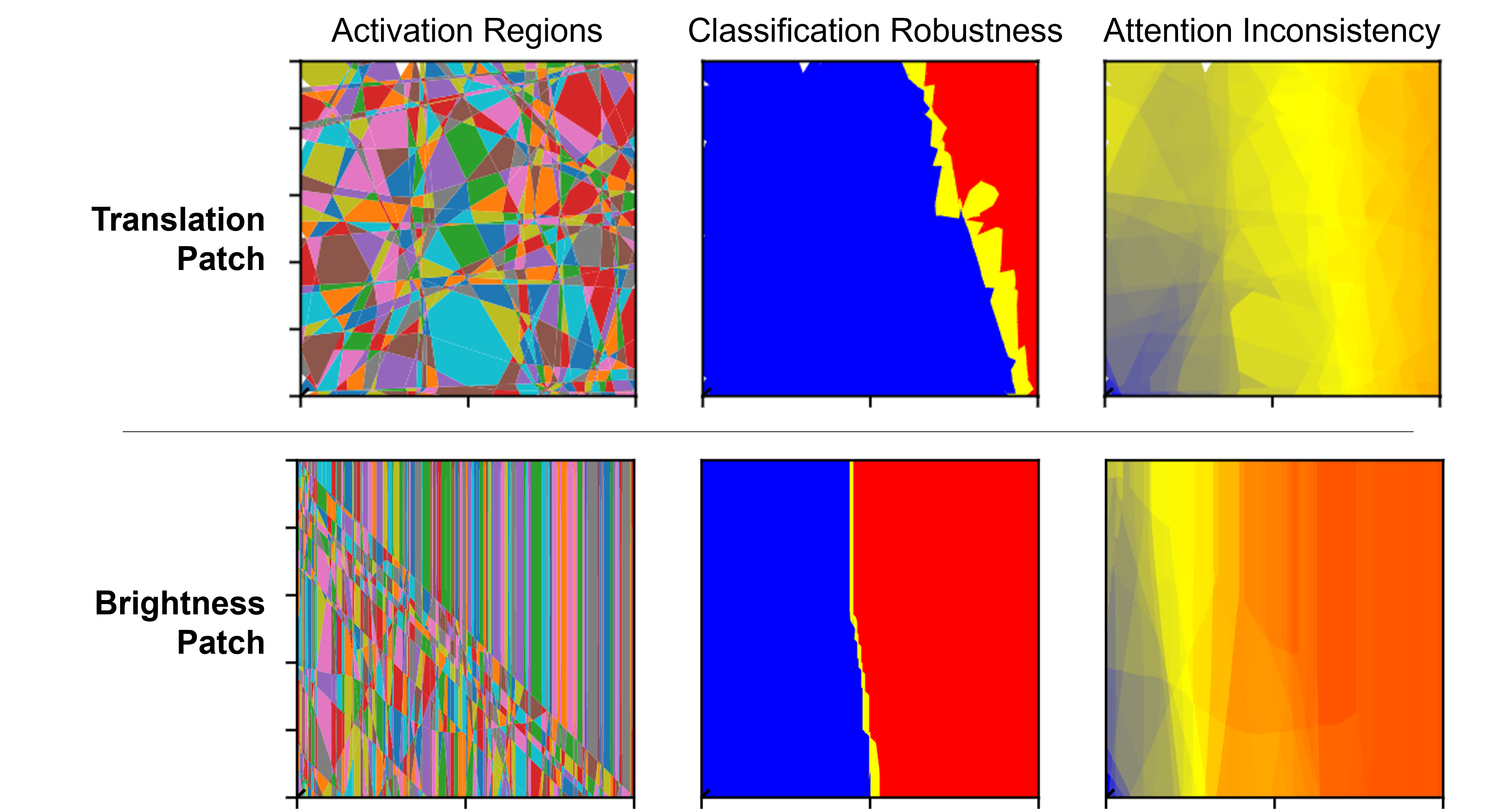
Case 1. Even if the brightness changes so much that the image is not visible to humans, the classification label of the perturbed image may happen to match the original label. Then vast ranges of the perturbation parameters are evaluated as robust for classification; however, such overestimated ranges are naturally invalid and unsafe. For instance, Figure 4 shows the changes in MNIST image “8” and the actual saliency-map when the brightness is gradually changed; although the classification seems robust because the labels of each image are the same, the collapsed saliency-maps indicate that the DNN does not pay proper attention to text “8” in each image. Therefore, our approach uses the metric attention inconsistency, which quantifies the degree of collapse of a saliency-map, to further evaluate the range of the perturbation parameter as satisfying the property attention robustness; i.e., the DNN is paying proper attention as well as the original image. Attention inconsistency is a kind of distance (cf. Figure 4) between an actual saliency-map (second row) and an expected one (third row); e.g., the saliency-map of DNN-1 for translation perturbation (column (T)) is expected to follow image translation; however, if it is not, then attention inconsistency is high. In addition, Figure 4 shows an example of determining that attention robustness is satisfied if each attention inconsistency value (third row) is less than or equal to threshold value .
Case 2. The classification label often changes by combining semantic perturbations, such as brightness change and patch, even for the perturbation parameter ranges that each perturbation alone could be robust. It is important to understand what combinations are weak for the DNN; however, it is difficult to verify all combinations as there are many semantic perturbations assumed in an operational environment. In our observations, a perturbation that significantly collapses the saliency-map is more likely to cause misclassification when combined with another perturbation because another perturbation can change the intensity of pixels to which the DNN should not pay attention. Therefore, to understand the weakness of combining perturbations, our approach visualizes the outermost boundary at which the sufficiency of robustness switches on the perturbation parameter space. For instance, Figure 4 shows connected regions that contain the outermost boundary for classification robustness (left side) or attention robustness (right side). The classification boundary indicates that the DNN can misclassify the image with a thin patch and middle brightness. In contrast, the attention boundary further indicates that the brightness change can collapse the saliency-map more than patching, so we can see that any combinations with the brightness change pose a greater risk. Even when the same perturbations are given, the values of attention inconsistency for different DNNs are usually different (cf. Figure 4); thus, it is better to evaluate what semantic perturbation poses a greater risk for each DNN.
3 Problem Formulation
Our method targets feed-forward ReLU-activated neural networks (ReLU-FNNs) for image classification. A ReLU-FNN image classifier is a function mapping an -dimensional (pixels color-depth) image to a classification label in the -class label space , where is the confidence function for the j-th class.
The ReLU activation function occurs in between the linear maps performed by the ReLU-FNN layers and applies the function to each neuron in a layer (where is the number of layers of ReLU-FNN ). When , we say that is active; otherwise, we say that is inactive. We write for the activation pattern of an image given as input to a ReLU-FNN , i.e., the sequence of neuron activation statuses in when is taken as input. We write for the entire set of activation patterns of a ReLU-FNN .
Given an activation pattern , we write for the corresponding activation region, i.e., the subset of the input space containing all images that share the same activation pattern: . Note that, neuron activation statuses in an activation pattern yield half-space constraints in the input space [9, 12]. Thus, an activation region can equivalently be represented as a convex polytope described by the conjunction of the half-space constraints resulting from the activation pattern .
3.0.1 Classification Robustness.
A semantic perturbation is a function applying a perturbation with parameters to an image to yield a perturbed image , where performs the -th atomic semantic perturbation with parameter (with for any image ). For instance, a brightness decrease perturbation is a(n atomic) semantic perturbation function with a single brightness adjustment parameter : .
Definition 1 (Classification Robustness)
A perturbation region satisfies classification robustness — written — if and only if the classification label is the same as when the perturbation parameter is within : .
Vice versa, we define misclassification robustness when is always different from when is within : .
The classification robustness verification problem consists in enumerating, for a given input image , the perturbation parameter regions respectively satisfying and .
3.0.2 Attention Robustness.
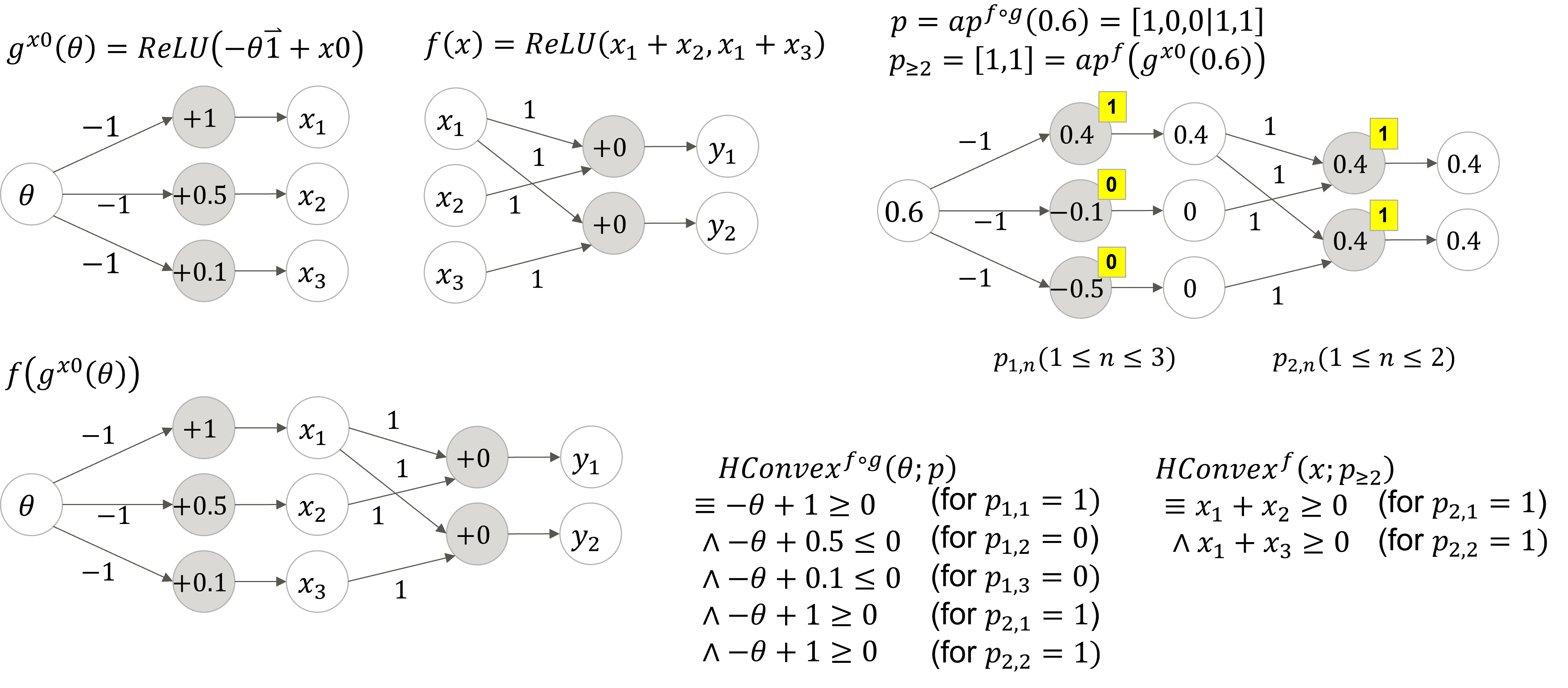
We generalize the definition of saliency-map from [21] to that of an attention-map, which is a function from an image to the heatmap image plotting the magnitude of the contribution to the j-th class confidence for each pixel of . Specifically, , where is an arbitrary image processing function (such as normalization and smoothing) and, following [21, 28], the magnitude of the contribution of each pixel is given by the gradient with respect to the -th class confidence. When , our definition of matches that of saliency-map in [21]. Note that, within an activation region , is linear [9] and thus the gradient is a constant value.
We expect attention-maps to change consistently with respect to a semantic image perturbation. For instance, for a brightness change perturbation, we expect the attention-map to remain the same. Instead, for a translation perturbation, we expect the attention-map to be subject to the same translation. In the following, we write for the attention-map perturbation corresponding to a given semantic perturbation . We define attention inconsistency as the difference between the actual and expected attention-map after a semantic perturbation:
where is an arbitrary distance function such as Lp-norm (). Note that, when is L2-norm, our definition of attention inconsistency coincides with the definition of saliency-map consistency given by [7].
Definition 2 (Attention Robustness)
A perturbation region satisfies attention robustness — written — if and only if the attention inconsistency is always less than or equal to when the perturbation parameter is within : .
When the attention inconsistency is always greater than , we have inconsistency robustness: .
The attention robustness verification problem consists in enumerating, for a given input image , the perturbation parameter regions respectively satisfying and .
3.0.3 Outermost Boundary Verification.
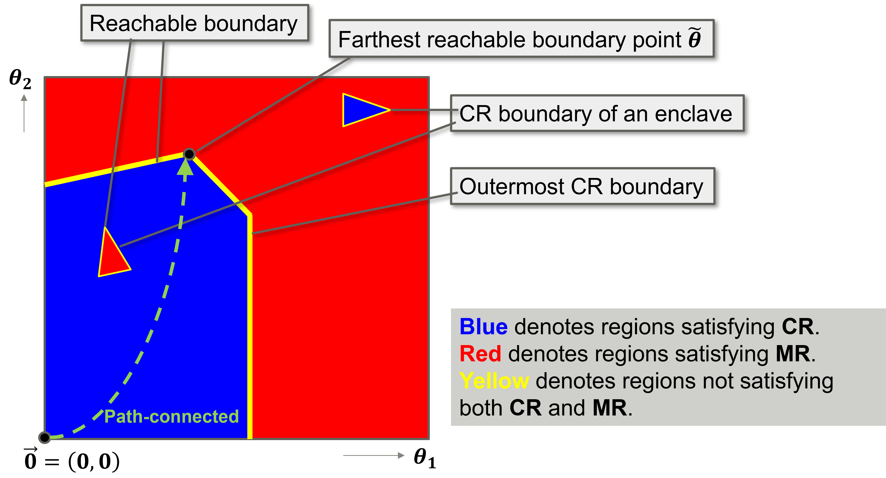
In practice, to represent the trend of the weakness of a ReLU-FNN image classifier to a semantic perturbation, we argue that it is not necessary to enumerate all perturbation parameter regions within a perturbation parameter space . Instead, we search the outermost / boundary, that is, the perturbation parameter regions that lay on the / boundary farthest away from the original image.
An illustration of the outermost CR boundary is given in Figure 5. More formally, we define the outermost boundary as follows:
Definition 3 (Outermost Boundary)
The outermost boundary of a classification robustness verification problem, , is a set of perturbation parameter regions such that:
-
1.
for all perturbation regions , there exists a path connected-space from the original image (i.e., ) to that consists of regions satisfying (written );
-
2.
all perturbation regions lay on the classification boundary, i.e., ;
-
3.
there exists a region that contains the farthest reachable perturbation parameter point from the original image, i.e., such that .
The definition of the outermost boundary is analogous. Note that not all perturbation regions inside the outermost / boundary satisfy the / property (cf. the enclaves in Figure 5).
The outermost boundary verification problem and outermost boundary verification problem and consist in enumerating, for a given input image , the perturbation parameter regions and ) that belong to the outermost and boundary and .
4 Geometric Boundary Search (GBS)
In the following, we describe our Geometric Boundary Search (GBS) method for solving , and shown in Algorithm 1 and 2. In Appendix I.8, we also describe our Breadth-First Search (BFS) method for solving , and .
4.1 Encoding Semantic Perturbations
After some variables initialization (cf. Line 1 in Algorithm 1), the semantic perturbation is encoded into a ReLU-FNN (cf. Line 2).
In this paper, we focus on combinations of atomic perturbations such as brightness change (B), patch placement (P), and translation (T). Nonetheless, our method is applicable to any semantic perturbation as long as it can be represented or approximated with sufficient accuracy.
For the encoding, we follow [16] and represent (combinations of) semantic perturbations as a piecewise linear function by using affine transformations and ReLUs. For instance, a brightness decrease perturbation (cf. Section 3.0.1) can be encoded as a ReLU-FNN as follows:
which we can combine with the given ReLU-FNN to obtain the compound ReLU-FNN to verify. The full encoding for all considered (brightness, patch, translation) perturbations is shown in Appendix I.5.
4.2 Traversing Activation Regions.
GBS then performs a traversal of activation regions of the compound ReLU-FNN near the outermost / boundary for /. Specifically, it initializes a queue with the activation pattern of the original input image with no semantic perturbation, i.e., (cf. Line 3 in Algorithm 1, we explain the other queue initialization parameters shortly). Given a queue element , the functions , , and respectively return the 1st, 2nd, and 3rd element of .
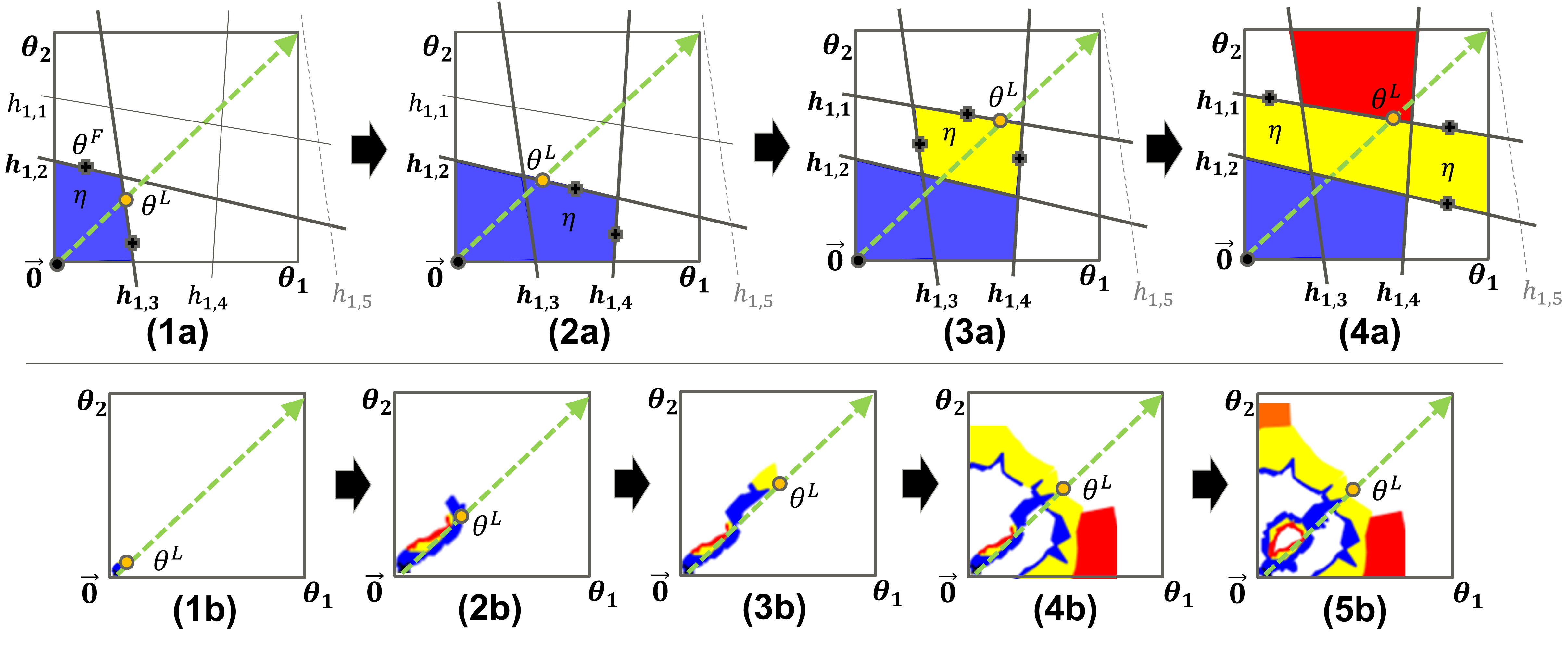
Then, for each activation pattern in (cf. Line 6), GBS reconstructs the corresponding perturbation parameter region (subroutine constructActivationRegion, Line 7) as the convex polytope resulting from (cf. Section 3 and in Figure 6-(1a)).
Next, for each neuron in (cf. Line 11), it checks whether its activation status cannot flip within the perturbation parameter space , i.e., the resulting half-space has no feasible points within (subroutine isStable, Line 12, cf. half-space in Figure 6-(1a)). Otherwise, a new activation pattern is constructed by flipping the activation status of (subroutine flipped, Line 13) and added to a local queue (cf. Line 9, and 23, 25) if has not been observed already (cf. Line 14) and it is feasible (subroutine calcInteriorPointOnFace, Lines 15-16. cf. point and half-space in Figure 6-(1a)).
The perturbation parameter region is then simplified to (subroutine simplified, Line 2 in Algorithm 2; e.g., reducing the half-spaces used to represent to just and in Figure 6-(1a)). is used to efficiently calculate the range of attention inconsistency within (subroutine calcRange, Line 3 in Algorithm 2, cf. Section 4.4), and then attention/inconsistency robustness can be verified based on the range (Line 5 and 8 in Algorithm 2). Furthermore, classification/misclassification robustness can be verified in the same way if subroutine returns the range of confidence within (cf. Section 4.4) and . At last, the local queue is pushed onto (cf. Line 29 in Algorithm 1).
To avoid getting stuck around enclaves inside the outermost / boundary (cf. Figure 5) during the traversal of activation regions, GBS switches status when needed between “searching for a decision boundary” and “following a found decision boundary”. The initial status is set to “searching for a decision boundary”, i.e., when initializing the queue (cf. Line 3). The switch to happens when region is on the boundary (i.e., ) or near the boundary (i.e., , cf. Line 15 in Algorithm 2 and Figure 6-(3a,1b,3b)); where is a hyperparameter to determine whether close to the boundary or not. should be greater than to verify attention/inconsistency robustness because attention inconsistency changes discretely for ReLU-FNNs (ch. Section 4.3). GBS can revert back to searching for a decision boundary if when following a found boundary it finds a reachable perturbation parameter region that is farther from (cf. Lines 19-20 in Algorithm 1 and Figure 6-(2b)).
4.3 Calculating Attention Inconsistency
Gradients within an Activation Region. Let be an activation pattern of the compound ReLU-FNN . The gradient is constant within (cf. Section 3.0.2). We write for the -th pixel of a perturbed image in . The gradient is also a constant value. By the chain rule, we have . Thus is also constant. This fact is formalized by the following lemma:
Lemma 1
(cf. a small example in Appendix I.7). Therefore, the gradient can be computed as the weights of the j-th class output for ReLU-FNN about activation pattern ; where, and is an arbitrary sample within (cf. Appendix I.1).
For the perturbed gradient , let be the ReLU-FNN . Thus, the same consideration as above applies.
Attention Inconsistency (ai). We assume both and are convex downward functions for calculating the maximum / minimum value by convex optimization. Specifically, is one of the identity function (I), the absolute function (A), and the mean filter (M). is one of the -norm () and the -norm (): where, is the width of image .
4.4 Verifying CR and AR within an activation region
Our method leverages the fact that the gradient of a ReLU-FNN output with respect to the input is constant within an activation region (cf. Section 3.0.2); thus, can be resolved by linear programming, and can be resolved by just only one sampling if the saliency-map is expected to keep or convex optimization if the saliency-map is expected to move.
Verifying CR/MR. When is fixed, each activation region of the ReLU-FNN is a region in the perturbation parameter space . Within an activation region of the ReLU-FNN , is satisfied if and only if the ReLU-FNN output corresponding to the label of the original image cannot be less than the ReLU-FNN outputs of all other labels, i.e., the following equation holds: Each DNN output is linear within , and thus, the left-hand side of the above equation can be determined soundly and completely by using an LP solver (Eq. 3-(c) in Appendix I.1), such as scipy.optimize.linprog 111https://docs.scipy.org/doc/scipy/reference/generated/scipy.optimize.linprog.html. Similarly, is satisfied if and only if the ReLU-FNN output corresponding to the label of the original image cannot be greater than the ReLU-FNN outputs of any other labels.
Verifying AR/IR. Within an activation region of the ReLU-FNN , is satisfied if and only if the following equation holds: If and are both convex downward functions, as the sum of convex downward functions is also a convex downward function, the left-hand side of the above equation can be determined by comparing the values at both ends. On the other hand, is satisfied if and only if the following equation holds: The left-hand side of the above equation can be determined by using an convex optimizer, such as scipy.optimize.minimize 222https://docs.scipy.org/doc/scipy/reference/generated/scipy.optimize.minimize.html Note that if the saliency-map is expected to keep against perturbations, the above optimization is unnecessary because is constant.
5 Experimental Evaluation
To confirm the usefulness of our method, we conducted evaluation experiments.
Setups. Table 1 shows the ReLU-FNNs for classification used in our experiments; each FNN uses different training data and architectures. We inserted semantic perturbation layers (cf. Section 4.1) in front of each ReLU-FNN for classification during each experiment; the layers had total 1,568 neurons.
| Name | #Neurons | Layers |
|---|---|---|
| M-FNN-100 | 100 | FC2 |
| M-FNN-200 | 200 | FC4 |
| M-FNN-400 | 400 | FC8 |
| M-FNN-800 | 800 | FC16 |
| M-CNN-S | 2,028 | Conv2,FC1 |
| M-CNN-M | 14,824 | Conv2,FC1 |
| Name | #Neurons | Layers |
|---|---|---|
| F-FNN-100 | 100 | FC2 |
| F-FNN-200 | 200 | FC4 |
| F-FNN-400 | 400 | FC8 |
| F-FNN-800 | 800 | FC16 |
| F-CNN-S | 2,028 | Conv2,FC1 |
| F-CNN-M | 14,824 | Conv2,FC1 |
All experiments were performed on virtual computational resource “rt_C.small” (with CPU 4 Threads and Memory 30 GiB) of physical compute node “V” (with 2 CPU; Intel Xeon Gold 6148 Processor 2.4 GHz 20 Cores (40 Threads), and 12 Memory; 32 GiB DDR4 2666 MHz RDIMM (ECC)) in AI Bridging Cloud Infrastructure (ABCI) 333https://docs.abci.ai/en/system-overview/ provided by National Institute of Advanced Industrial Science and Technology (AIST).
We implemented our method in a python tool for evaluation; in addition, we will make the tool available at https://zenodo.org/record/6544905 444However, due to our internal procedures, we cannot publish it until at least May 21..
RQ1: How much computation time is required to solve each problem? For each ReLU-FNN, we measured the computation time of algorithms GBS and BFS with 10 images selected from the end of each dataset (i.e., Indexes 69990-69999. These images were not used in the training of any ReLU-FNNs). GBS also distinguishes between gbs-CR that traverses the CR boundary, gbs-AR that traverses the AR boundary, and gbs-CRAR that traverses the boundary of the regions satisfying both CR and AR. Furthermore, we measured above per the combinations of semantic perturbations (BP), (TP), and (TB) that denote “brightness change / patch”, “translation / patch”, and “translation / brightness change”, respectively. We used the definitions , , , and .
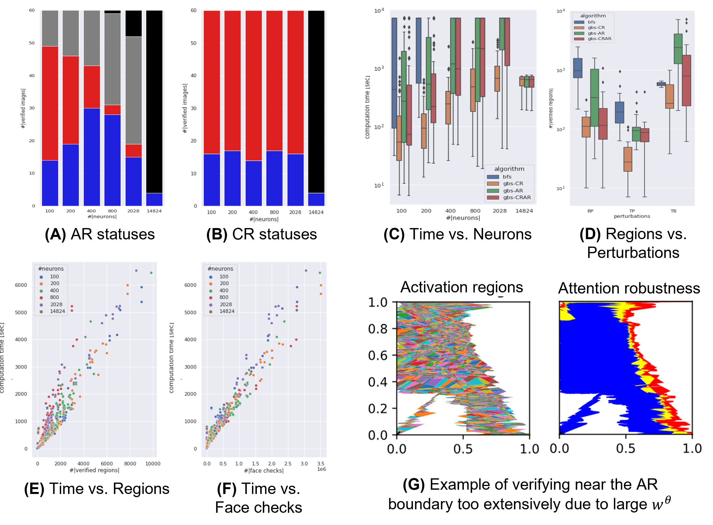
Figure 7-(C) shows the trend of increasing computation time with increasing the number of neurons for each algorithm as a box plot on a log scale. Note that each verification timed out at 2 hours, and thus, the upper limit of computation time (y-axis) was 7,200 seconds. We can see that algorithm BFS took more computation time than GBS. Figure 7-(D) shows the number of verified activation regions for each combination of perturbations; we can see that GBS reduced the number of regions to traverse compared to BFS as intended.
However, we can also see that gbs-AR took longer to traverse more activation regions than gbs-CR. Figure 7-(A) and (B) show the breakdown of each verification result for gbs-AR and gbs-CR; where, blue, red, gray, and black bars denote robust, not-robust, timed out, and out-of-memory, respectively. The figures show that gbs-AR timed out at a higher rate for smaller size DNNs than gbs-CR.
Moreover, we can also see that the median computation time increased exponentially with the number of neurons for all algorithms in Figure 7-(C). This result suggests that exact verification-based traversing is not applicable to practical-scale DNNs such as VGG16[22], and fundamental scalability improvement measures, such as incorporating approximate verification, are needed.
RQ2: What are the performance factors? Figure 7-(E) and (F) show the correlation between computation time and the number of verified activation regions and the number of face checking as scatter plots, respectively: where the results of experiments that timed out are excluded. The figures show strong positive correlations for each DNN size (the number of neurons), especially in the number of face checking; thus, reducing redundant regions and faces in understanding the boundaries should directly reduce verification time. For example, Figure 7-(G) shows an example of verifying activation regions near the AR boundary too extensively due to large hyperparameter . Like gbs-CR, AR boundary also needs to be able to narrow down the search to only the regions on the AR boundaries.
6 Discussion
Internal Validity. Using the outermost / boundary as a trend of weakness to a combination of semantic perturbations, not all regions inside the outermost / boundary satisfy the / property. Unlike , requires hyperparameters ; however, there are no clear criteria for setting them.
External Validity. We focus here on brightness change, patch, and translation perturbations. Still, our method applies to any semantic perturbations as long as they can be represented or approximated with sufficient accuracy. Our method is not applicable to a semantic perturbation for which a corresponding saliency-map change cannot be defined and computed, e.g., DNNs that generate an image from an input text (such as [18]). Our method has not supported the MaxPool layer of CNNs[13].
Performance Bottlenecks.
The computation time increases exponentially with the number of ReLU-FNN neurons. Thus, our current method is not yet applicable on a practical scale, such as VGG16 [22]. If it is difficult to enumerate all activation regions, GBS traverses only regions on the outermost boundary. In the future, it may be better to use ReLU relaxation for dense areas.
7 Related Work
Robustness Verification. To the best of our knowledge, there have been no reports that formulate the attention robustness verification problem or that propose the method for such problem; e.g., [11, 30, 1]. [23] first verified robustness against image rotation, and [2] verified robustness against more semantic perturbations, such as image translation, scaling, shearing, brightness change, and contrast change. However, in this paper, we have demonstrated that attention robustness more accurately captures trends in weakness for the combinations of semantic perturbations than existing classification robustness in some cases. In addition, As [25] reported, approximated verification methods like DeepPoly[23] fail to verify near the boundary. In contrast, our GBS enables verification near the boundary by exploratory and exact verification.
[16] proposed that any Lp-norm-based verification tools can be used to verify the classification robustness against semantic perturbations by inserting special DNN layers that induce semantic perturbations in the front of DNN layers for classification. In order to transform the verification problem on the inherently high-dimensional input image space into one on the low-dimensional perturbation parameter space , we adopted their idea, i.e., inserting DNN layers for semantic perturbations () in front of DNN layers for classification (). However, it is our original idea to calculate the value range of the gradient for DNN output () within an activation region on the perturbation parameter space (cf. Sections 4.3-4.4).
Traversing activation regions. Since [12] first proposed the method to traverse activation regions, several improvements and extensions have been proposed [14, 5]. All of them use all breadth-first searches with a priority queue to compute the maximum safety radius or the maxima of the given objective function in fewer iterations. In contrast, our algorithm GBS uses a breadth-first search with a priority queue to reach the outermost / boundary in fewer iterations while avoiding enclaves.
[5] responded to the paper reviewer that traversing time would increase exponentially with the size of a DNN 555https://openreview.net/forum?id=zWy1uxjDdZJ. Our experiment also showed that larger DNNs increase traversing time due to the denser activation regions. The rapid increase in the number of activation regions will be one of the biggest barriers to the scalability of traversing methods, including our method. Although the upper bound theoretical estimation for the number of activation regions increases exponentially with the number of layers in a DNN [10], [9] reported that actual DNNs have surprisingly few activation regions because of the myriad of infeasible activation patterns. Therefore, it will need to understand the number of activation regions of DNNs operating in the real world.
To improve scalability, there is the method of dividing the input space and verifying each in perfectly parallel [29]. However, our method has not been fully parallelized yet, because we have focused on accurately calculating the outermost / boundary and attention robustness in this study. To improve scalability, there are several methods of targeting only low-dimensional subspaces in the high-dimensional input space for verification [24, 26, 15]. We have similarly taken advantage of low-dimensionality, e.g., using low-dimensional perturbation parameters to represent high-dimensional input image pixels as mediator variables (i.e., curried perturbation function ) to reduce the elapsed time of LP solvers, determining the stability of neuron activity from few vertices of perturbation parameter space .
Saliency-Map. Since [21] first proposed the method to obtain a saliency-map from the gradients of DNN outputs with respect to an input image (i.e., ), many improvements and extensions have been proposed [3, 27, 20]. We formulated an attention-map primarily using the saliency-map definition by [21]. However, it is a future work to formulate attention robustness corresponding to improvements, such as gradient-smoothing[3] and line-integrals [27].
It is known that semantic perturbations can significantly change the saliency-maps [17, 7, 8]. [7] first claimed the saliency-map should consistently follow image translation and proposed the method to quantify saliency-map consistency. We formulated attention inconsistency primarily using the saliency-map consistency by [7].
8 Conclusion and Future Work
We, for the first time, have presented a verification method for attention robustness based on traversing activation regions on the DNN that contains layers for semantic perturbations and layers for classification. Attention robustness is the property that the saliency-map consistency is less than a threshold value. We have demonstrated that attention robustness more accurately captures trends in weakness for the combinations of semantic perturbations than existing classification robustness. Although the performance evaluation presented in this study is not yet on a practical scale, such as VGG16 [22], we believe that the attention robustness verification problem we have formulated opens a new door to quality assurance for DNNs. We plan to increase the number of semantic perturbation types that can be verified and improve scalability by using abstract interpretation in future work.
References
- [1] Ashmore, R., Calinescu, R., Paterson, C.: Assuring the machine learning lifecycle: Desiderata, methods, and challenges. ACM Computing Surveys (CSUR) 54(5), 1–39 (2021)
- [2] Balunovic, M., Baader, M., Singh, G., Gehr, T., Vechev, M.: Certifying geometric robustness of neural networks. In: NeurIPS. vol. 32 (2019)
- [3] Daniel, S., Nikhil, T., Been, K., Fernanda, V., Wattenberg, M.: Smoothgrad: removing noise by adding noise. In: ICMLVIZ. PMLR (2017)
- [4] Engstrom, L., Tran, B., Tsipras, D., Schmidt, L., Madry, A.: Exploring the landscape of spatial robustness. In: ICML. pp. 1802–1811. PMLR (2019)
- [5] Fromherz, A., Leino, K., Fredrikson, M., Parno, B., Pasareanu, C.: Fast geometric projections for local robustness certification. In: ICLR. ICLR (2021)
- [6] Gao, X., Saha, R.K., Prasad, M.R., Roychoudhury, A.: Fuzz testing based data augmentation to improve robustness of deep neural networks. In: ICSE. pp. 1147–1158. IEEE,ACM (2020)
- [7] Guo, H., Zheng, K., Fan, X., Yu, H., Wang, S.: Visual attention consistency under image transforms for multi-label image classification. In: CVPR. pp. 729–739. IEEE,CVF (2019)
- [8] Han, T., Tu, W.W., Li, Y.F.: Explanation consistency training: Facilitating consistency-based semi-supervised learning with interpretability. In: AAAI. vol. 35, pp. 7639–7646. AAAI (2021)
- [9] Hanin, B., Rolnick, D.: Deep relu networks have surprisingly few activation patterns. In: NeurIPS. vol. 32 (2019)
- [10] Hinz, P.: An analysis of the piece-wise affine structure of ReLU feed-forward neural networks. Ph.D. thesis, ETH Zurich (2021)
- [11] Huang, X., Kroening, D., Ruan, W., Sharp, J., Sun, Y., Thamo, E., Wu, M., Yi, X.: A survey of safety and trustworthiness of deep neural networks: Verification, testing, adversarial attack and defence, and interpretability. Computer Science Review 37, 100270 (2020)
- [12] Jordan, M., Lewis, J., Dimakis, A.G.: Provable certificates for adversarial examples: Fitting a ball in the union of polytopes. In: NeurIPS. vol. 32 (2019)
- [13] Krizhevsky, A., Sutskever, I., Hinton, G.E.: Imagenet classification with deep convolutional neural networks. In: NeurIPS. vol. 25 (2012)
- [14] Lim, C.H., Urtasun, R., Yumer, E.: Hierarchical verification for adversarial robustness. In: ICML. vol. 119, pp. 6072–6082. PMLR (2020)
- [15] Mirman, M., Hägele, A., Bielik, P., Gehr, T., Vechev, M.: Robustness certification with generative models. In: PLDI. pp. 1141–1154. ACM SIGPLAN (2021)
- [16] Mohapatra, J., Weng, T.W., Chen, P.Y., Liu, S., Daniel, L.: Towards verifying robustness of neural networks against a family of semantic perturbations. In: CVPR. pp. 244–252. IEEE,CVF (2020)
- [17] Montavon, G., Samek, W., Müller, K.R.: Methods for interpreting and understanding deep neural networks. Digital Signal Processing 73, 1–15 (2018)
- [18] Ramesh, A., Pavlov, M., Goh, G., Gray, S., Voss, C., Radford, A., Chen, M., Sutskever, I.: Zero-shot text-to-image generation. In: ICML. PMLR (2021)
- [19] Ribeiro, M.T., Singh, S., Guestrin, C.: “why should i trust you?” explaining the predictions of any classifier. In: KDD. pp. 1135–1144. ACM SIGKDD (2016)
- [20] Selvaraju, R.R., Cogswell, M., Das, A., Vedantam, R., Parikh, D., Batra, D.: Grad-cam: Visual explanations from deep networks via gradient-based localization. In: ICCV. IEEE (Oct 2017)
- [21] Simonyan, K., Vedaldi, A., Zisserman, A.: Deep inside convolutional networks: Visualising image classification models and saliency maps. In: ICLR (2014)
- [22] Simonyan, K., Zisserman, A.: Very deep convolutional networks for large-scale image recognition. In: ICLR (2015)
- [23] Singh, G., Gehr, T., Püschel, M., Vechev, M.: An abstract domain for certifying neural networks. In: POPL. pp. 1–30. ACM New York, NY, USA (2019)
- [24] Sotoudeh, M., Thakur, A.V.: Computing linear restrictions of neural networks. In: NeurIPS. vol. 32 (2019)
- [25] Sotoudeh, M., Thakur, A.V.: Provable repair of deep neural networks. In: PLDI. pp. 588–603. ACM SIGPLAN (2021)
- [26] Sotoudeh, M., Thakur, A.V.: Syrenn: A tool for analyzing deep neural networks. In: TACAS. pp. 281–302 (2021)
- [27] Sundararajan, M., Taly, A., Yan, Q.: Axiomatic attribution for deep networks. In: ICML. pp. 3319–3328. PMLR (2017)
- [28] Tsipras, D., Santurkar, S., Engstrom, L., Turner, A., Madry, A.: Robustness may be at odds with accuracy. In: ICLR (2019)
- [29] Urban, C., Christakis, M., Wüstholz, V., Zhang, F.: Perfectly parallel fairness certification of neural networks. Proceedings of the ACM on Programming Languages 4(OOPSLA), 1–30 (2020)
- [30] Urban, C., Miné, A.: A review of formal methods applied to machine learning. CoRR abs/2104.02466 (2021), https://arxiv.org/abs/2104.02466
I Appendix
I.1 Linearity of Activation Regions
Given activation pattern as constant, within activation region each output of ReLU-FNN is linear for (cf. Figure 8) because all ReLU operators have already resolved to or [9]. i.e., : where, and denote simplified weights and bias about activation pattern and class .
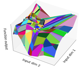
ReLU-FNN output is linear on each activation region, i.e., each output plane painted for each activation region is flat.
That is, the gradient of each ReLU-FNN output within activation region is constant, i.e., the following equation holds: where is a constant value.
| (1) |
An activation region can be interpreted as the H-representation of a convex polytope on input space . Specifically, neuron activity and have a one-to-one correspondence with a half-space and convex polytope defined by the intersection (conjunction) of all half-spaces, because is also linear when is constant. Therefore, we interpret activation region and the following H-representation of convex polytope each other as needed: where, and denote simplified weights and bias about activation pattern , and is the half-space corresponding to the n-th neuron activity in the l-th layer.
| (2) |
I.2 Connectivity of Activation Regions
When feasible activation patterns are in a relationship with each other that flips single neuron activity , they are connected regions because they share single face corresponding to flipped [12]. It is possible to flexibly traverse activation regions while ensuring connectivity by selecting a neuron activity to be flipped according to a prioritization; several traversing methods have been proposed [12, 14, 5]. However, there are generally rather many neuron activities that become infeasible when flipped [12]. For instance, half-spaces is a face of activation region in Figure 6-(1a); thus, flipping neuron activity , GBS can traverse connected region in Figure 6-(1b). In contrast, half-space is not a face of activation region in Figure 6-(1a); thus, flipping neuron activity , the corresponded activation region is infeasible (i.e., the intersection of flipped half-spaces has no area).
I.3 Hierarchy of Activation Regions
When feasible activation patterns are in a relationship with each other that matches all of -th upstream activation pattern , they are included parent activation region corresponding to convex polytope [14]. That is, and .
Similarly, we define -th downstream activation pattern as .
I.4 Linear Programming on an Activation Region
Based on the linearity of activation regions and ReLU-FNN outputs, we can use Linear Programming (LP) to compute (a) the feasibility of an activation region, (b) the flippability of a neuron activity, and (c) the minimum (maximum) of a ReLU-FNN output within an activation region. We show each LP encoding of the problems (a,b,c) in the SciPy LP form 666https://docs.scipy.org/doc/scipy/reference/generated/scipy.optimize.linprog.html: where, is a given activation pattern of ReLU-FNN , and is a give neuron activity to be flipped.
| (3) |
I.5 Full Encoding Semantic Perturbations
. We focus here on the perturbations of brightness change (B), patch (P), and translation (T), and then describe how to encode the combination of them into ReLU-FNN : where, , is the width of image , are the patch x-position, y-position, width, height, and is the amount of movement in x-axis direction. Here, perturbation parameter consists of the amount of brightness change for (B), the density of the patch for (P), and the amount of translation for (T). In contrast, perturbation parameters not included in the dimensions of , such as , are assumed to be given as constants before verification.
I.6 Images used for our experiments
We used 10 images (i.e., Indexes 69990-69999) selected from the end of the MNIST dataset (cf. Figure 10) and the Fashion-MNIST dataset (cf. Figure 10), respectively. We did not use these images in the training of any ReLU-FNNs.
![[Uncaptioned image]](https://cdn.awesomepapers.org/papers/3594e465-0818-47fe-bb4a-2f3787aff9a7/MNIST_i69990-69999.png)
|
![[Uncaptioned image]](https://cdn.awesomepapers.org/papers/3594e465-0818-47fe-bb4a-2f3787aff9a7/Fashion-MNIST_i69990-69999.png)
|
I.7 An example of Lemma 1
Lemma 1 is reprinted below.
A small example of Lemma 1 (cf. Figure 11)
Let , , , , , and .
Because and , .
Then, .
Here, corresponding to , on the other hand, corresponding to .
Because , .
I.8 Algorithm BFS
Algorithm BFS traverses entire activation regions in perturbation parameter space , as shown in Figure 12.
Algorithm BFS initializes with (Line 3). Then, for each activation pattern in (Lines 5-6), it reconstructs the corresponding activation region (subroutine constructActivationRegion, Line 8) as the H-representation of (cf. Equation 2). Next, for each neuron in (Line 12), it checks whether the neuron activity cannot flip within the perturbation parameter space , i.e., one of the half-spaces has no feasible points within (subroutine isStable, Line 13). Otherwise, a new activation pattern is constructed by flipping (subroutine flipped, Line 14) and added to the queue (Line 20) if is feasible (subroutine calcInteriorPointOnFace, Lines 17-18). Finally, the activation region is simplified (Line 24) and used to verify (subroutine solveCR and solveVR, Lines 25-27, cf. Section 4.4) and (subroutine solveAR and solveIR, Lines 32-34, cf. Section 4.4).
I.9 Details of experimental results
Table 2 shows breakdown of verification statuses in experimental results for each algorithm and each DNN size (cf. Section 5). In particular, for traversing AR boundaries, we can see the problem that the ratio of “Timeout” and “Failed (out-of-memory)” increases as the size of the DNN increases. This problem is because gbs-AR traverses more activation regions by the width of the hyperparameter than gbs-CR. It would be desirable in the future, for example, to traverse only the small number of activation regions near the AR boundary.
| algorithm | #neurons | Robust | NotRobust | Timeout | Failed |
|---|---|---|---|---|---|
| bfs | 100 | 13 | 22 | 25 | 0 |
| bfs | 200 | 11 | 15 | 34 | 0 |
| gbs-CR | 100 | 16 | 44 | 0 | 0 |
| gbs-CR | 200 | 17 | 43 | 0 | 0 |
| gbs-CR | 400 | 14 | 46 | 0 | 0 |
| gbs-CR | 800 | 17 | 43 | 0 | 0 |
| gbs-CR | 2028 | 16 | 44 | 0 | 0 |
| gbs-CR | 14824 | 4 | 0 | 0 | 56 |
| gbs-AR | 100 | 14 | 35 | 11 | 0 |
| gbs-AR | 200 | 19 | 27 | 14 | 0 |
| gbs-AR | 400 | 30 | 13 | 17 | 0 |
| gbs-AR | 800 | 28 | 3 | 28 | 1 |
| gbs-AR | 2028 | 15 | 4 | 33 | 8 |
| gbs-AR | 14824 | 4 | 0 | 0 | 56 |
| gbs-CRAR | 100 | 14 | 41 | 5 | 0 |
| gbs-CRAR | 200 | 19 | 33 | 8 | 0 |
| gbs-CRAR | 400 | 30 | 14 | 16 | 0 |
| gbs-CRAR | 800 | 28 | 6 | 26 | 0 |
| gbs-CRAR | 2028 | 15 | 8 | 32 | 5 |
| gbs-CRAR | 14824 | 4 | 0 | 0 | 56 |