VHE -ray emission of PKS 2155304:
spectral and temporal variability
Abstract
Context. Observations of very high energy -rays from blazars provide information about acceleration mechanisms occurring in their innermost regions. Studies of variability in these objects allow a better understanding of the mechanisms at play.
Aims. To investigate the spectral and temporal variability of VHE () -rays of the well-known high-frequency-peaked BL Lac object PKS 2155304 with the H.E.S.S. imaging atmospheric Cherenkov telescopes over a wide range of flux states.
Methods. Data collected from 2005 to 2007 are analyzed. Spectra are derived on time scales ranging from 3 years to 4 minutes. Light curve variability is studied through doubling timescales and structure functions, and is compared with red noise process simulations.
Results. The source is found to be in a low state from 2005 to 2007, except for a set of exceptional flares which occurred in July 2006. The quiescent state of the source is characterized by an associated mean flux level of above , or approximately of the Crab Nebula, and a power law photon index of . During the flares of July 2006, doubling timescales of are found. The spectral index variation is examined over two orders of magnitude in flux, yielding different behaviour at low and high fluxes, which is a new phenomenon in VHE -ray emitting blazars. The variability amplitude characterized by the fractional r.m.s. is strongly energy-dependent and is . The light curve r.m.s. correlates with the flux. This is the signature of a multiplicative process which can be accounted for as a red noise with a Fourier index of .
Conclusions. This unique data set shows evidence for a low level -ray emission state from PKS 2155304, which possibly has a different origin than the outbursts. The discovery of the light curve lognormal behaviour might be an indicator of the origin of aperiodic variability in blazars.
Key Words.:
gamma rays: observations – Galaxies : active – Galaxies : jets – BL Lacertae objects: individual objects: PKS 21553041 Introduction
The BL Lacertae (BL Lac) category of Active Galactic Nuclei (AGN) represents the vast majority of the population of energetic and extremely variable extragalactic very high energy -ray emitters. Their luminosity varies in unpredictable, highly irregular ways, by orders of magnitude, and at all wavelengths across the electromagnetic spectrum. The very high energy (VHE, ) -ray fluxes vary often on the shortest timescales that can be seen in this type of object, with large amplitudes which can dominate the overall output. It hence indicates that the understanding of this energy domain is the most important one for understanding the underlying fundamental variability and emission mechanisms at play in high flux states.
It has been, however, difficult to ascertain whether -ray emission is present only during high flux states or also when the source is in a more stable or quiescent state but with a flux which is below the instrumental limits. The advent of the current generation of atmospheric Cherenkov telescopes with unprecedented sensitivity in the VHE regime gives new insights into these questions.
The high frequency peaked BL Lac object (HBL) PKS 2155304, located at a redshift , initially discovered as a VHE -ray emitter by the Mark 6 telescope (Chadwick et al. (1999)), has been detected by the first H.E.S.S. telescope in 2002-2003 (Aharonian et al. 2005b). It has been frequently observed by the full array of four telescopes since 2004, either sparsely during the H.E.S.S. monitoring program, or intensely during dedicated campaigns such as that described in Aharonian et al. (2005c), showing mean flux levels of of the Crab Nebula flux for energies above . During the summer of 2006, PKS 2155304 exhibited unprecedented flux levels accompanied by strong variability (Aharonian et al. 2007a), making temporal and spectral variability studies possible on timescales of the order of a few minutes. The VHE -ray emission is usually thought to originate from a relativistic jet, emanating from the vicinity of a Supermassive Black Hole (SMBH). The physical processes at play are still poorly understood, but the analysis of the -ray flux spectral and temporal characteristics is well suited to provide better insights.
For this goal the data set of H.E.S.S. observations of PKS 2155304 between 2005 and 2007 is used. After describing the observations and the analysis chain in Section 2, the emission from the “quiescent”, i.e. nonflaring, state of the source will be characterized in Section 3. Section 4 details spectral variability related to the source intensity. Section 5 will focus on the description of the temporal variability during the highly active state of the source, and its possible energy dependence. Section 6 will illustrate a description of the observed variability phenomenon by a random stationary process, characterized by a simple power density spectrum. Section 7 will show how limits on the characteristic time of the source can be derived. The multi-wavelength aspects from the high flux state will be presented in a second paper.
2 Observations and analysis
H.E.S.S. is an array of four imaging atmospheric Cherenkov telescopes situated in the Khomas Highland of Namibia ( South, East), at an elevation of 1,800 meters above sea level (see Aharonian et al. 2006). PKS 2155304 was observed by H.E.S.S. each year since 2002; results of observations in 2002, 2003 and 2004 can be found in Aharonian et al. (2005b), Aharonian et al. (2005c) and Giebels et al. (2005). The data reported here were collected between 2005 and 2007. In 2005, 12.2 hours of observations were taken. A similar observation time was scheduled in 2006, but following the strong flare of July 26th (Aharonian et al. 2007a) it was decided to increase this observation time significantly. Ultimately, from June to October 2006, this source was observed for 75.9 hours, with a further 20.9 hours in 2007.
| Year | Excess | |||||
|---|---|---|---|---|---|---|
| 2005 | 9.4 | 7,282 | 27,071 | 1,868 | 21.8 | 7.1 |
| 2006 | 66.1 | 123,567 | 203,815 | 82,804 | 288.4 | 35.5 |
| 2007 | 13.8 | 11,012 | 40,065 | 2,999 | 28.6 | 7.7 |
| Total | 89.2 | 141,861 | 270,951 | 87,671 | 275.6 | 29.2 |
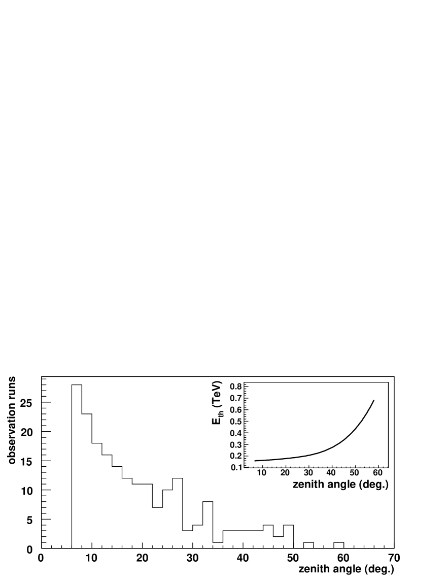
The data have been recorded during runs of 28 minutes nominal duration, with the telescopes pointing at from the source position in the sky to enable a simultaneous estimate of the background. This offset has been taken alternatively in both right ascension and declination (with both signs), in order to minimize systematics. Only the runs passing the H.E.S.S. data-quality selection criteria have been used for the analyses presented below. These criteria imply good atmospheric conditions and checks that the hardware state of the cameras is satisfactory. The number of runs thus selected is 22 for 2005, 153 for 2006 and 35 for 2007, corresponding to live-times of 9.4, 66.1 and 13.8 hours respectively. During these observations, zenith angles were between 7 and 60 degrees, resulting in large variations in the instrument energy threshold (, see Fig. 1) and sensitivity. This variation has been accounted for in the spectral and temporal variability studies presented below.
The data have been analysed following the prescription presented in Aharonian et al. (2006), using the loose set of cuts which are well adapted for bright sources with moderately soft spectra, and the Reflected-Region method for the definition of the on-source and off-source data regions. A year-wise summary of the observations and the resulting detections are shown in Table 1. A similar summary is given in Appendix A for the 67 nights of data taken, showing that the emission of PKS 2155304 is easily detected by H.E.S.S. almost every night. For 66 nights out of 67, the significance per square root of the live-time (, where is the observation live-time) is at least equal to , the only night with a lower value — MJD 53705 — corresponding to a very short exposure. In addition, for 61 nights out of 67 the source emission is high enough to enable a detection of the source with 5 significance in one hour or less, a level usually required in this domain to firmly claim a new source detection. In 2006 the source exhibits very strong activity (38 nights, between MJD 53916 – 53999) with a nightly varying from 3.6 to 150, and being higher than for 19 nights. The activity of the source climaxes on MJD 53944 and 53946 with statistical significances which are unprecedented at these energies, the rate of detected -rays corresponding to 2.5 and , with 150 and respectively.
For subsequent spectral analysis, an improved energy reconstruction method with respect to the one described in Aharonian et al. (2006) was applied. This method is based on a look-up table determined from Monte-Carlo simulations, which contains the relation between an image’s amplitude and its reconstructed impact parameter as a function of the true energy, the observation zenith angle, the position of the source in the camera, the optical efficiency of the telescopes (which tend to decrease due to the aging of the optical surfaces), the number of triggered telescopes and the reconstructed altitude of the shower maximum. Thus, for a given event, the reconstructed energy is determined by requiring the minimal between the image amplitudes and those expected from the look-up table corresponding to the same observation conditions. This method yields a slightly lower energy threshold (shown in Fig. 1 as a function of zenith angle), an energy resolution which varies from 15% to 20% over all the energy range, and biases in the energy reconstruction which are smaller than 5%, even close to the threshold. The systematic uncertainty in the normalization of the H.E.S.S. energy scale is estimated to be as large as 15%, corresponding for such soft spectrum source to 40% in the overall flux normalization as quoted in Aharonian et al. (2009).
All the spectra presented in this paper have been obtained using a forward-folding maximum likelihood method based on the measured energy-dependent on-source and off-source distributions. This method, fully described in Piron et al. (2001), performs a global deconvolution of the instrument functions (energy resolution, collection area) and the parametrization of the spectral shape. Two different sets of parameters, corresponding to a power law and to a power law with an exponential cut-off, are used for the spectral shape, with the following equations :
| (1) | |||||
| (2) | |||||
represents the differential flux at (chosen to be 1 TeV), is the power law index and the characteristic energy of the exponential cut-off. The maximum likelihood method provides the best set of parameters corresponding to the selected hypothesis, and the corresponding error matrix.
| Label | Period | Runs | (hours) | Excess | Section | Additional criteria | |
|---|---|---|---|---|---|---|---|
| 2005–2007 | 165 | 69.7 | 67,654 | 237.4 | 4, 7 | – | |
| 2005–2007 | 115 | 48.1 | 12,287 | 60.5 | 3.2, 3.4, 3.3, 7 | July 2006 excluded | |
| 2005 | 19 | 8.0 | 1,816 | 22.6 | 3.4 | – | |
| 2006 | 61 | 26.3 | 7,472 | 48.4 | 3.4 | July 2006 excluded | |
| 2007 | 35 | 13.8 | 2,999 | 28.6 | 3.4 | – | |
| July 2006 | 50 | 21.6 | 55,367 | 281.8 | 4, 5, 6, 7 | – | |
| July 2006 (4 nights) | 27 | 11.8 | 46,036 | 284.1 | 4, 5, 6, 7 | – |
Finally, various data sets have been used for subsequent analyses. These are summarized in Table 2.
3 Characterization of the quiescent state
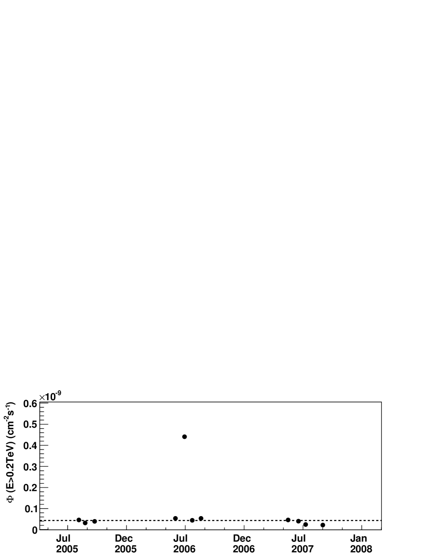
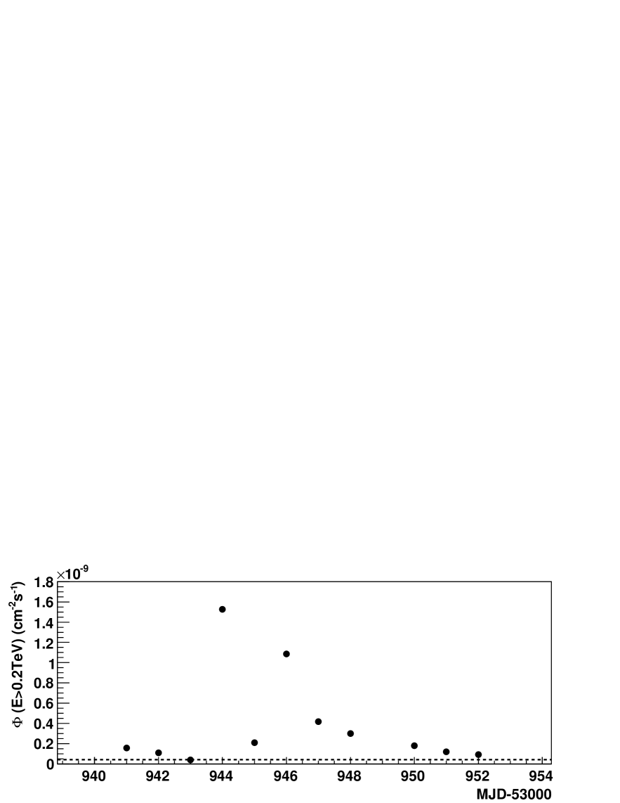
As can be seen in Fig. 2, with the exception of the high state of July 2006 PKS 2155304 was in a low state during the observations from 2005 to 2007. This section explores the variability of the source during these periods of low-level activity, based on the determination of the run-wise integral fluxes for the data set , which excludes the flaring period of July 2006 and also those runs whose energy threshold is higher than (see 3.1 for justification). As for Sections 5 and 6, the control of systematics in such a study is particularly important, especially because of the strong variations of the energy threshold throughout the observations.
3.1 Method and systematics
The integral flux for a given period of observations is determined in a standard way. For subsequent discussion purposes, the formula applied is given here :
| (3) |
where represents the corresponding live-time, and are, respectively, the collection area at the true energy and the energy resolution function between and the measured energy , and the shape of the differential energy spectrum as defined in Eq. 1 and 2 . Finally, is the number of measured events in the energy range [Emin,Emax].
In the case that is a power law, an important source of systematic error in the determination of the integral flux variation with time comes from the value chosen for the index . The average 2005–2007 energy spectrum yields a very well determined power law index111 The average 2005–2007 energy spectrum yields a power law with a photon index . One should note that some curvature is observed at higher energies, resulting in a better spectral determination when the alternative hypothesis shown in (Eq. 2) is used, yielding a harder index () with an exponential cut-off at energy . This curved model is prefered at a level as compared to the power law hypothesis. However, the choice of the model has little effect on the determination of the integral flux values above , the integral being dominated by the low-energy part of the energy spectrum.. However, in Section 4 it will be shown that this index varies depending on the flux level of the source. Moreover, in some cases the energy spectrum of the source shows some curvature in the TeV region, giving slight variations in the fitted power law index depending on the energy range used.
For runs whose energy threshold is lower than , a simulation performed under the observation conditions corresponding to the data shows that an index variation of implies a flux error at the level of , this relation being quite linear up to . However, this relation no longer holds when the energy threshold is above , as the determination of becomes much more dependent on the choice of . For this reason, only runs whose energy threshold is lower than will be kept for the subsequent light curves. The value of is chosen as , which is a compromise between a low value which maximises the excess numbers used for the flux determinations and a high value which maximises the number of runs whose energy threshold is lower than .
3.2 Run-wise distribution of the integral flux
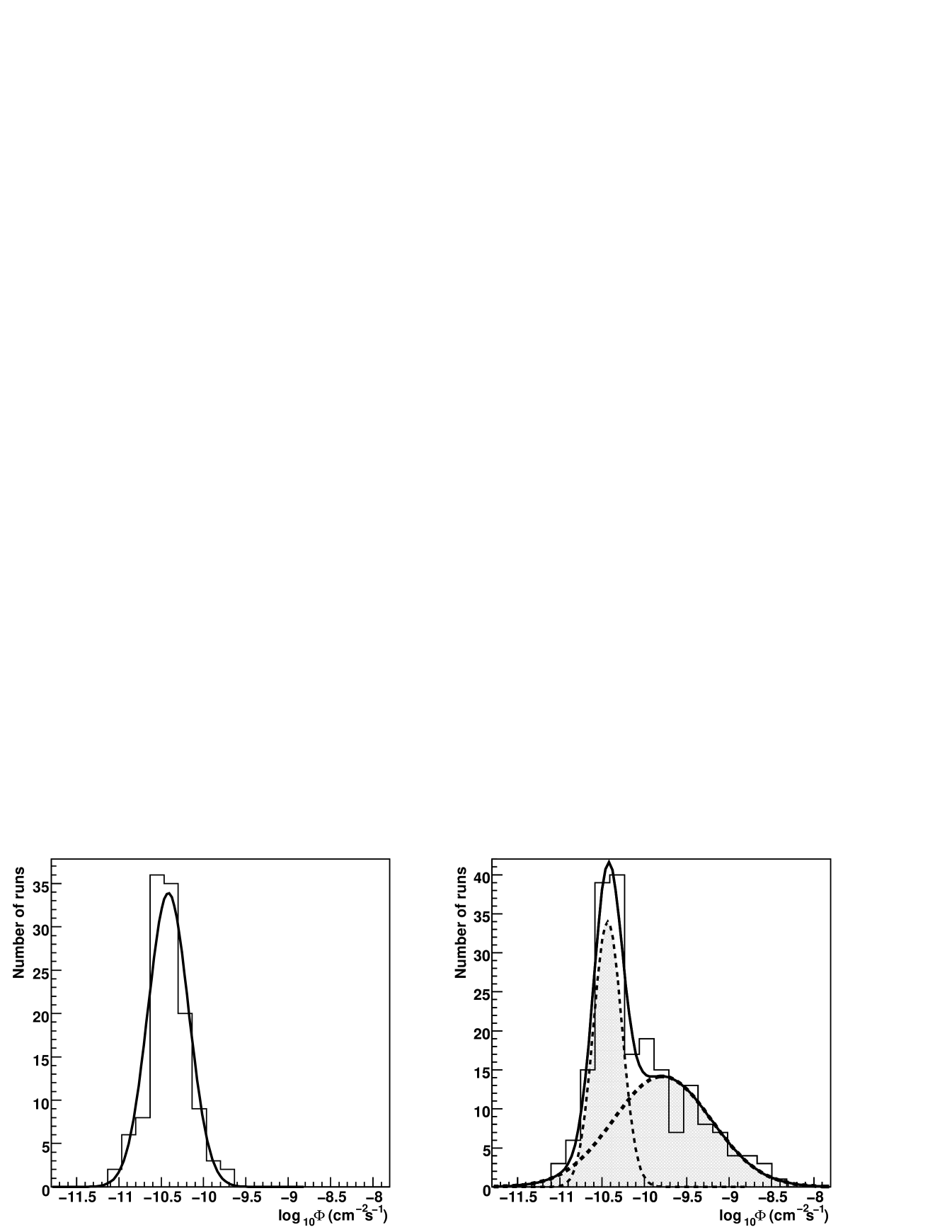
From 2005 to 2007, PKS 2155304 is almost always detected when observed (except for two nights for which the exposure was very low), indicating the existence, at least during these observations, of a minimal level of activity of the source. Focussing on data set (which excludes the July 2006 data where the source is in a high state), the distribution of the integral fluxes of the individual runs above has been determined for the 115 runs, using a spectral index (the best value for this data set, as shown in 3.4). This distribution has an asymmetric shape, with mean value and root mean square (r.m.s.) , and is very well described with a lognormal function. Such a behaviour implies that the logarithm of fluxes follows a normal distribution, centered on the logarithm of . This is shown in the left panel of Fig. 3, where the solid line represents the best fit obtained with a maximum-likelihood method, yielding results independent of the choice of the intervals in the histogram. It is interesting to note that this result can be compared to the fluxes measured by H.E.S.S. from PKS 2155304 during its construction phase, in 2002 and 2003 (see Aharonian et al. 2005b and Aharonian et al. 2005c). As shown in Table 3, these flux levels extrapolated down to were close to the value corresponding to the peak shown in the left panel of Fig. 3.
| Month | Year | [] |
|---|---|---|
| July | 2002 | |
| Oct. | 2002 | |
| June | 2003 | |
| July | 2003 | |
| Aug. | 2003 | |
| Sep. | 2003 | |
| Oct. | 2003 |
The right panel of Fig. 3 shows how the flux distribution is modified when the July 2006 data are taken into account (data set in Table 2): the histogram can be accounted for by the superposition of two Gaussian distributions (solid curve). The results, summarized in Table 4, are also independent of the choice of the intervals in the histogram. Remarkably enough, the characteristics of the first Gaussian obtained in the first step (left panel) remain quite stable in the double Gaussian fit.
| “Quiescent” regime | Flaring regime | |
|---|---|---|
| -10.42 0.02 | -9.79 0.11 | |
| r.m.s. | 0.24 0.02 | 0.58 0.04 |
This leads to two conclusions. First, the flux distribution of PKS 2155304 is well described considering
a low state and a high state, for each of which the distribution of the logarithms of the fluxes follows
a Gaussian distribution. The characteristics of the lognormal flux distribution for the high state
are given in Sections 5, 6 and 7.
Secondly, PKS 2155304 has a level of minimal
activity which seems to be stable on a several-year time-scale. This state will henceforth be
referred to as the “quiescent state” of the source.
3.3 Width of the run-wise flux distribution
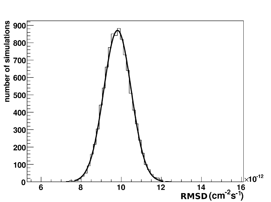
In order to determine if the measured width of the flux distribution (left panel of Fig. 3) can be explained as statistical fluctuations from the measurement process a simulation has been carried out considering a source which emits an integral flux above of with a power law photon spectrum index (as determined in the next section). For each run of the data set the number expected by convolving the assumed differential energy spectrum with the instrument response corresponding to the observation conditions is determined. A random smearing around this value allows statistical fluctuations to be taken into account. The number of events in the off-source region and also the number of background events in the source region are derived from the measured values in the data set. These are also smeared in order to take into account the expected statistical fluctuations.
10000 such flux distributions have been simulated, and for each one its mean value and r.m.s. (which will be called below RMSD) are determined. The distribution of RMSD thus obtained, shown in Fig. 4, is well described by a Gaussian centred on (which represents a relative flux dispersion of 23%) and with a of .
It should be noted that here the effect of atmospheric fluctuations in the determination of the flux is only taken into account at the level of the off-source events, as these numbers are taken from the measured data. But the effect of the corresponding level of fluctuations on the source signal is very difficult to determine. If a conservative value of 20% is considered 222 A similar procedure has been carried out on the Crab Nebula observations. Considering this source to be perfectly stable it allows us to determine an upper limit to the fluctuations of the Crab signal due to the atmosphere, and a value of was derived. Nonetheless, this value is linked to the observations’ epoch and zenith angles, and to the source spectral shape. , which is added in the simulations as a supplementary fluctuation factor for the number of events expected from the source, a RMSD distribution centred on with a of is obtained. Even in this conservative case, the measured value for the flux distribution r.m.s. () is very far (more than 8 standard deviations) from the simulated value. All these elements strongly suggest the existence of an intrinsic variability associated with the quiescent state of PKS 2155304.
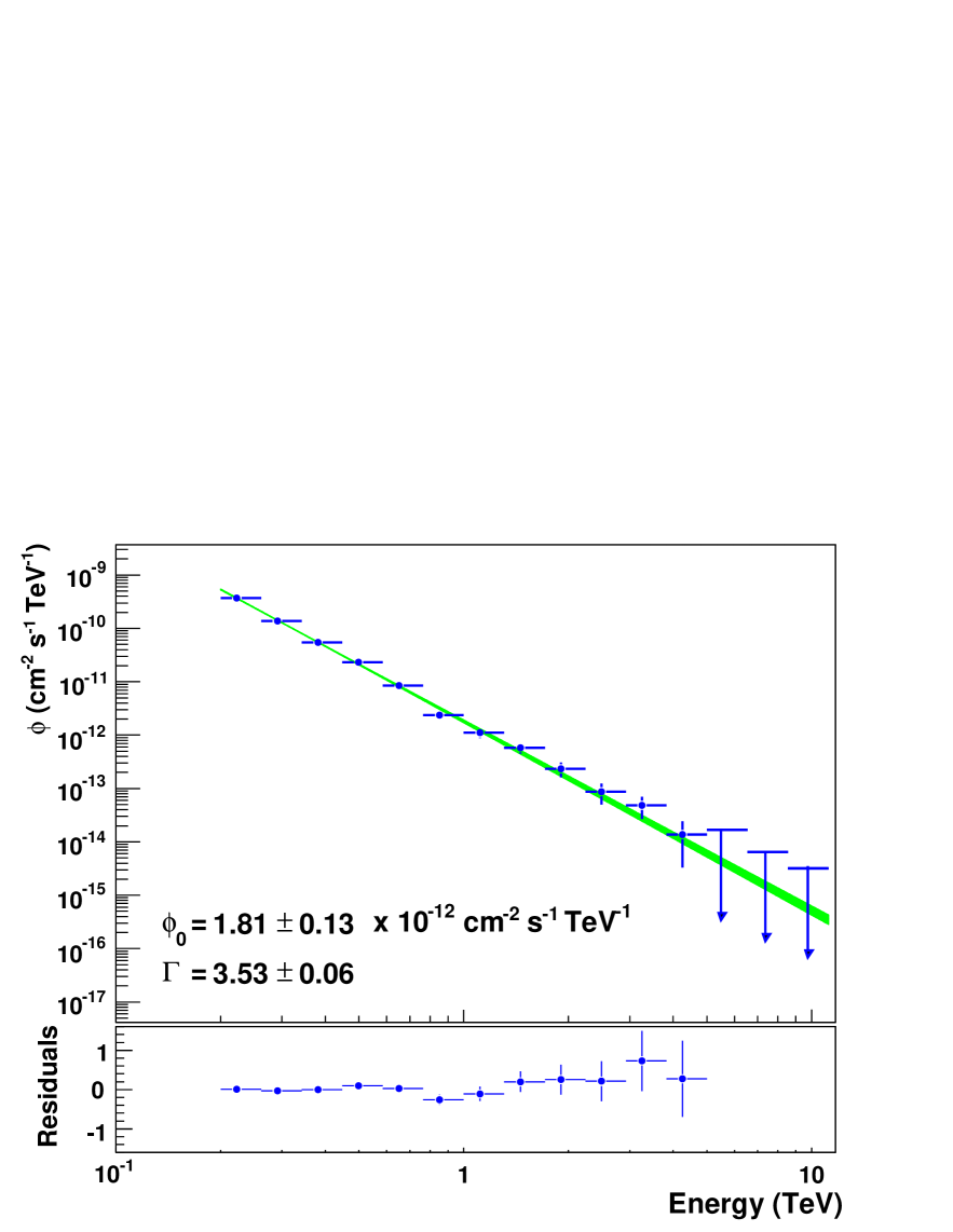
3.4 Quiescent-state energy spectrum
The energy spectrum associated with the data set , shown in Fig. 5, is well described by a power law with a differential flux at 1 TeV of and an index of . The stability of these values for spectra measured separately for 2005, 2006 (excluding July) and 2007 is presented in Table 5. The corresponding average integral flux is , which is as expected in very good agreement with the mean value of the distribution shown in the left panel of Fig. 3.
| Year | Data set | |||
|---|---|---|---|---|
| 2005–2007 | ||||
| 2005 | ||||
| 2006 | ||||
| 2007 |
Bins above 2 TeV correspond to ray excesses lower than 20 and significances lower than . Above 5 TeV excesses are even less significant ( or less) and 99% upper-limits are used. There is no improvement of the fit when a curvature is taken into account.
4 Spectral variability
4.1 Variation of the spectral index for the whole data set 2005-2007
The spectral state of PKS 2155304 has been monitored since 2002. The first set of observations (Aharonian et al. 2005b), from July 2002 to September 2003, shows an average energy spectrum well described by a power law with an index of , for an integral flux (extrapolated down to ) of . No clear indication of spectral variability was seen. Consecutive observations in October and November 2003 (Aharonian et al. 2005c) gave a similar value for the index, , for a slightly higher flux of . Later, during H.E.S.S. observations of the first (MJD 53944, Aharonian et al. 2007a) and second (MJD 53946, Aharonian et al. 2009) exceptional flares of July 2006, the source reached much higher average fluxes, corresponding to and 333corresponding to data set T200 in Aharonian et al. (2009) respectively. In the first case, no strong indications for spectral variability were found and the average index was close to those associated with the 2002 and 2003 observations. In the second case, clear evidence of spectral hardening with increasing flux was found.
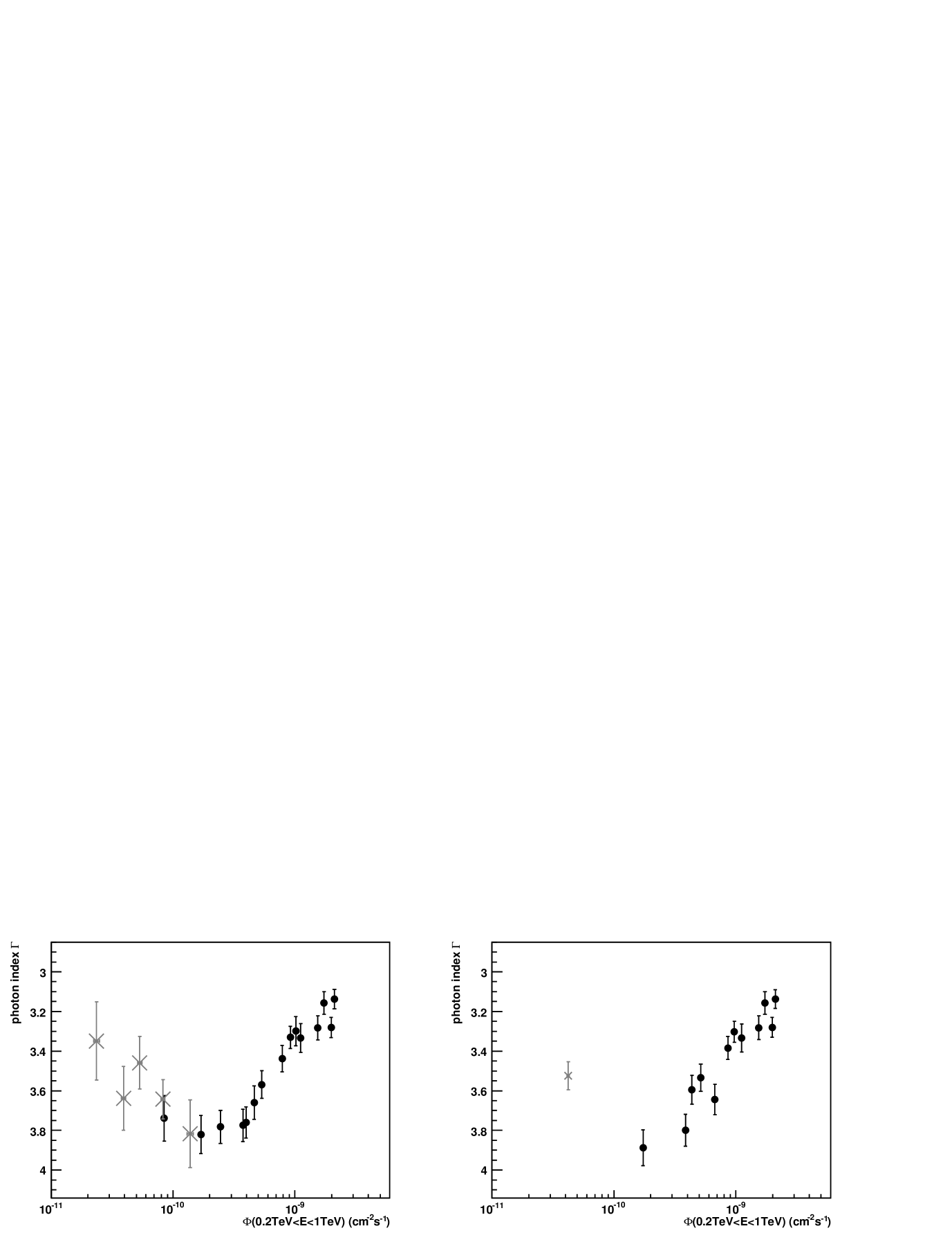
The observations of PKS 2155304 presented in this paper also include the subsequent flares of 2006 and the data of 2005 and 2007. Hence, the evolution of the spectral index is studied for the first time for a flux level varying over two orders of magnitude. This spectral study has been carried out over the fixed energy range 0.2–1 TeV in order to minimize both systematic effects due to the energy threshold variation and the effect of the curvature observed at high energy in the flaring states. The maximal energy has been chosen to be at the limit where the spectral curvature seen in high flux states begins to render the power law or exponential curvature hypotheses distinguishable. As flux levels observed in July 2006 are significantly higher than in the rest of the data set (see Fig. 6), the flux–index behaviour is determined separately first for the July 2006 data set itself () and secondly for the 2005-2007 data excluding this data set ().
On both data sets, the following method was applied. The integral flux was determined for each run assuming a power law shape with an index of (average spectral index for the whole data set), and runs were sorted by increasing flux. The set of ordered runs was then divided into subsets containing at least an excess of 1500 above and the energy spectrum of each subset was determined444even for lower fluxes, the significance associated with each subset is always higher than 20 standard deviations.
The left panel of Fig. 7 shows the photon index versus integral flux for data sets (grey crosses) and (black points). Corresponding numbers are summarized in Appendix B. While a clear hardening is observed for integral fluxes above a few , a break in this behaviour is observed for lower fluxes. Indeed, for the data set (black points) a linear fit yields a slope /, whereas the same fit for data set (grey crosses) yields a slope /. The latter corresponds to a probability ; a fit to a constant yields but with a constant fitted index incompatible with a linear extrapolation from higher flux states at a 3 level. This is compatible with conclusions obtained either with an independant analysis or when these spectra are processed following a different prescription. In this prescription the runs were sorted as a function of time in contiguous subsets with similar photon statistics, rather than as a function of increasing flux.
The form of the relation between the index versus integral flux is unprecedented in the TeV regime. Prior to the results presented here, spectral variability has been detected only in two other blazars, Mrk 421 and Mrk 501. For Mrk 421, a clear hardening with increasing flux appeared during the 1999/2000 and 2000/2001 observations performed with HEGRA (Aharonian et al. (2002)) and also during the 2004 observations performed with H.E.S.S. (Aharonian et al. 2005a ). In addition, the Mrk 501 observations carried out with CAT during the strong flares of 1997 (Djannati-Ataï et al. (1999)) and also the recent observation performed by MAGIC in 2005 (Albert et al. 2007) have shown a similar hardening. In both studies, the VHE peak has been observed in the distributions of the flaring states of Mrk 501.
4.2 Variation of the spectral index for the four flaring nights of July 2006
In this section, the spectral variability during the flares of July 2006 is described in more detail. A zoom on the variation of the integral flux (4-minute binning) for the four nights containing the flares (nights MJD 53944, 53945, 53946, and 53947, called the “flaring period”) is presented in the top panel of Fig. 8. This figure shows two exceptional peaks on MJD 53944 and MJD 53946 which climax respectively at fluxes higher than and ( and times the Crab Nebula level above the same energy), both about two orders of magnitude above the quiescent state level.
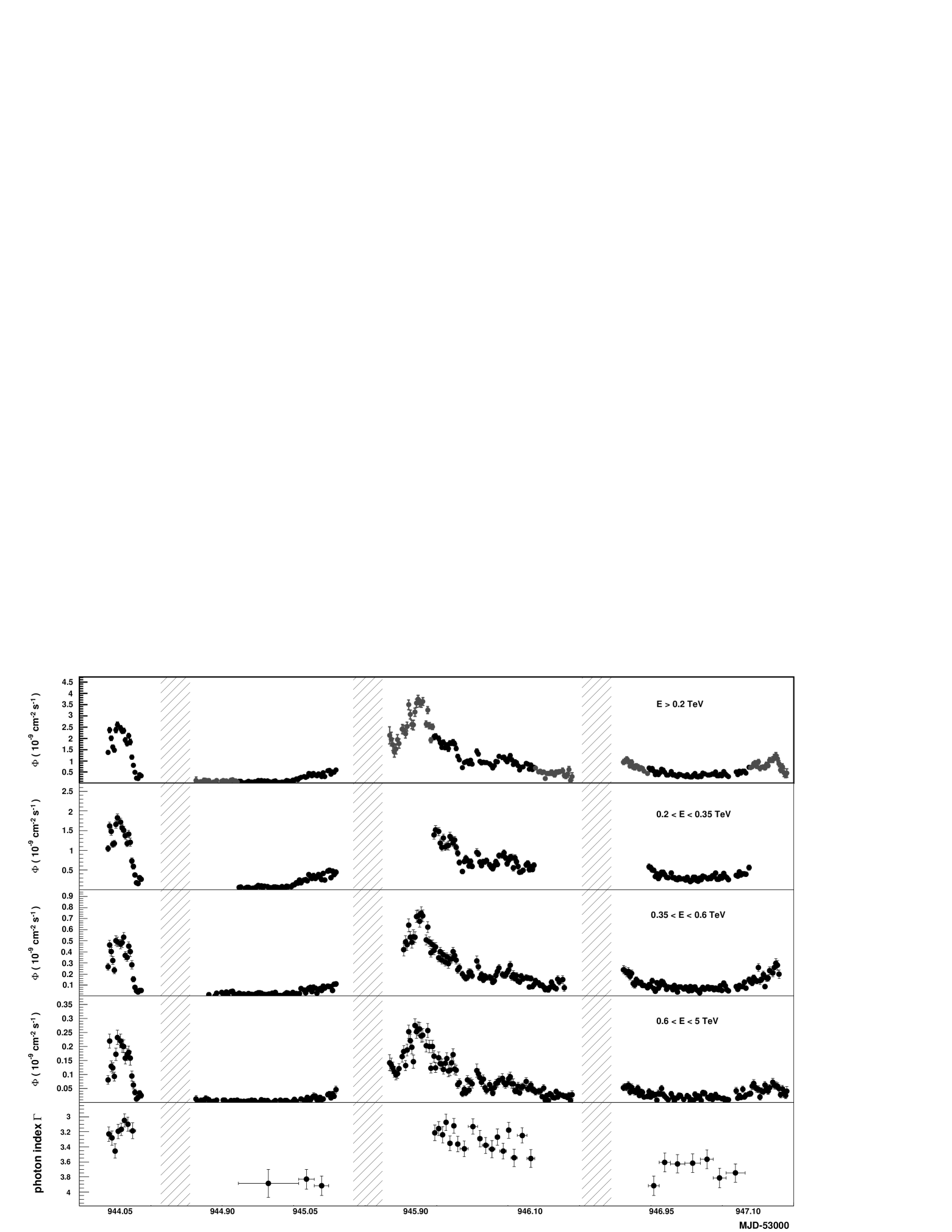
The variation with time of the photon index is shown in the bottom panel of Fig. 8. To obtain these values, the excess above has been determined for each 4-minute bin. Then, successive bins have been grouped in order to reach a global excess higher than 600 . Finally, the energy spectrum of each data set has been determined in the 0.2–1 TeV energy range, as before (corresponding numbers are summarized in Appendix Table 14). There is no clear indication of spectral variability within each night, except for MJD 53946 as shown in Aharonian et al. (2009). However, a variability can be seen from night to night, and the spectral hardening with increasing flux level already shown in Fig. 7 is also seen very clearly in this manner.
It is certainly interesting to directly compare the spectral behaviour seen during the flaring period with the hardness of the energy spectrum associated with the quiescent state. This is shown in the right panel of Fig. 7, where black points correspond to the four flaring nights; these were determined in the same manner as for the left panel (see 4.1 for details). A linear fit here yields a slope /. The grey cross corresponds to the integral flux and the photon index associated with the quiescent state (derived in a consistent way in the energy range from 0.2–1 TeV), showing a clear rupture with the tendancy at higher fluxes (typically above ).
These four nights were further examined to search for differences in the spectral behaviour between periods in which the source flux was clearly increasing and periods in which it was decreasing. For this, the first 16 minutes of the first flare (MJD 53944) are of special interest because they present a very symmetric situation: the flux increases during the first half, and then decreases to its initial level, the averaged fluxes are similar in both parts (), and the observation conditions (and thus the instrument response) are almost constant — the mean zenith angle of each part being respectively and degrees. Again, the spectra have been determined in the 0.2–1 TeV energy range, giving indices of and respectively. To further investigate this question and avoid potential systematic errors from the spectral method determination, the hardness ratios were derived (defined as the ratio of the excesses in different energy bands), using for this the energy (TeV) bands [0.2–0.35], [0.35–0.6] and [0.6–5.0]. For any combination, no differences were found beyond the level between the increasing and decreasing parts. A similar approach has been applied — when possible — for the rest of the flaring period. No clear dependence has been found within the statistical error limit of the determined indices, which is distributed between 0.09 and 0.20.
Finally, the persistence of the energy cut-off in the differential energy spectrum along the flaring period has been examined. For this purpose, runs were sorted again by increasing flux and grouped into subsets containing at least an excess of 3000 above 555To be significant, the determination of an energy cut-off needs a greater number of than for a power law fit.. For the seven subsets found, the energy spectrum has been determined in the 0.2–10 TeV energy range both for a simple power law and a power law with an exponential cut-off. This last hypothesis was found to be favoured systematically at a level varying from 1.8 to 4.6 compared to the simple power-law and is always compatible with a cut-off in the 1–2 TeV range.
5 Light curve variability and correlation studies
This section is devoted to the characterization of the temporal variability of PKS 2155304, focusing
on the flaring period observations. The high number of -rays available not only allowed
minute-level time scale studies, such as those presented for MJD 53944 in
Aharonian et al. (2007a), but also to derive detailed light curves for three energy bands (Fig. 8): 0.2–0.35 TeV,
0.35–0.6 TeV and 0.6–5 TeV.
The variability of the energy-dependent light curves of PKS 2155304 is in the following quantified through
their fractional r.m.s. defined in Eq. 4 (Nandra et al. (1997); Edelson et al. (2002)). In addition, possible time lags between light
curves in two energy bands are investigated.
5.1 Fractional r.m.s.
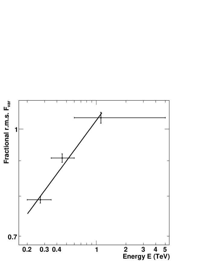
All fluxes in the energy bands of Fig. 8 show a strong variability which is quantified through their fractional r.m.s. (which depends on observation durations and their sampling). Measurement errors on each of the fluxes of the light curve are taken into account in the definition of :
| (4) |
where is the variance
| (5) |
and where is the mean square error and is the mean flux.
The energy-dependent variability has been calculated for the flaring period according to Eq. 4 in all three energy bands. The uncertainties on have been estimated according to the parametrization derived by Vaughan et al. (2003), using a Monte Carlo approach which accounts for the measurement errors on the simulated light curves.
Fig. 9 shows the energy dependence of over
the four nights for a sampling of 4 minutes where only fluxes with a
significance of at least 2 standard deviations were considered. There
is a clear energy-dependence of the variability (a null
probability of ). The points in Fig. 9
are fitted according to a power law showing that the variability follows
.
This energy dependence of is also perceptible within each individual night. In Table 6 the values of , the relative mean flux, and the observation duration, are reported night by night for the flaring period. Because of the steeply falling spectra, the low energy events dominate in the light curves. This lack of statistics for high energy prevents to have a high fraction of points with a significance more than 2 standard deviation in light curves night by night for the three energy bands previously considered. On the other hand, the error contribution dominates and does not allow to estimate the in all these three energy bands. Therefore, only two energy bands were considered: low (0.2–0.5 TeV) and high (0.5–5 TeV). As can be seen in Table 6 also night by night the high-energy fluxes seem to be more variable than those at lower energies.
| MJD | Duration | Energy | ||
|---|---|---|---|---|
| (min) | (TeV) | (10-10 ) | ||
| 53944 | 88 | |||
| all | 15.440.87 | 0.560.01 | ||
| 0.2 - 0.5 | 13.280.85 | 0.550.01 | ||
| 0.5 - 5.0 | 1.940.24 | 0.610.03 | ||
| 53945 | 244 | |||
| all | 2.400.41 | 0.670.03 | ||
| 0.2 - 0.5 | 2.350.42 | 0.640.03 | ||
| 0.5 - 5.0 | 0.340.12 | - | ||
| 53946 | 252 | |||
| all | 11.390.80 | 0.350.01 | ||
| 0.2 - 0.5 | 10.020.79 | 0.330.01 | ||
| 0.5 - 5.0 | 1.390.20 | 0.430.02 | ||
| 53947 | 252 | |||
| all | 4.260.52 | 0.220.02 | ||
| 0.2 - 0.5 | 4.020.52 | 0.220.02 | ||
| 0.5 - 5.0 | 0.370.11 | 0.130.09 |
5.2 Doubling/halving timescale
While characterizes the mean variability of a source, the shortest doubling/halving time (Zhang et al. 1999) is an important parameter in view of finding an upper limit on a possible physical shortest time scale of the blazar.
If represents the light curve flux at a time , for each
pair of one may calculate , where =-, =-
and . Two possible definitions of the
doubling/halving are proposed by Zhang et al. (1999): the smallest
doubling time of all data pairs in a light curve (), or the mean
of the 5 smallest (in the following indicated as
). One should keep in mind that, according
to Zhang et al. (1999), these quantities are ill defined and strongly depend on the length of the sampling intervals and on the signal-to-noise ratio in the observation.
This quantity was calculated for the two nights with the highest fluxes,
MJD 53944 and MJD 53946, considering light curves with two
different binnings (1 and 2 minutes). Bins with flux significances more than and flux ratios with an uncertainty smaller than 30% were
required to estimate the doubling time scale. The uncertainty on
was estimated by propagating the errors on the , and a dispersion of the 5 smallest values was included in the error for .
In Table 7, the values of and for the two nights are shown. The dependence with respect to the binning is clearly visible for both observables. In this table, the last column shows that the fraction of pairs in the light curves which are kept in order to estimate the doubling times is on average 45%. Moreover, doubling times and have been estimated for two sets of pairs in the light curves where =- is increasing or decreasing respectively. The values of the doubling time for the two cases are compatible within , therefore no significant asymmetry has been found.
| MJD | Bin size | [min] | [min] | Fraction of pairs |
|---|---|---|---|---|
| 53944 | 1 min | 1.650.38 | 2.270.77 | 0.53 |
| 53944 | 2 min | 2.200.60 | 4.451.64 | 0.62 |
| 53946 | 1 min | 1.610.45 | 5.723.83 | 0.25 |
| 53946 | 2 min | 4.551.19 | 9.154.05 | 0.38 |
It should be noted that these values are strongly dependent on the time binning and on the experiment’s sensitivity, so that the typical fastest doubling timescale should be conservatively estimated as being less than , which is compatible with the values reported in Aharonian et al. (2007a) and in Albert et al. (2007), the latter concerning the blazar Mrk 501.
5.3 Cross-correlation analysis as a function of energy
Time lags between light curves at different energies can provide insights into acceleration, cooling and propagation effects of the radiative particles.
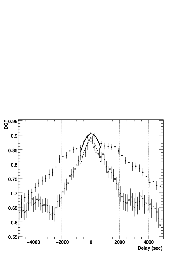
The Discrete Correlation Function (DCF) as a function of the delay (White & Peterson (1984); Edelson & Krolik (1988)) is used here to search for possible time lags between the energy-resolved light curves. The uncertainty on the DCF has been estimated using simulations. For each delay, light curves (in both energy bands) have been generated within their errors, assuming a Gaussian probability distribution. A probability distribution function (PDF) of the correlation coefficients between the two energy bands has been estimated for each set of simulated light curves. The r.m.s. of these PDF are the errors related to the DCF at each delay. Fig. 10 shows the DCF between the high and low energy bands for the four-night flaring period (with 4 minute bins) and for the second flaring night (with 2 minute bins). The gaps between each 28 minute run have been taken into account in the DCF estimation.
The position of the maximum of the DCF has been estimated by a Gaussian fit, which shows no time lag between low and high energies for either the 4 or 2 minute binned light curves. This sets a limit of from the observation of MJD 53946. A detailed study on the limit on the energy scale on which quantum gravity effects could become important, using the same data set, are reported in Aharonian et al. (2008a).
5.4 Excess r.m.s.–flux correlation
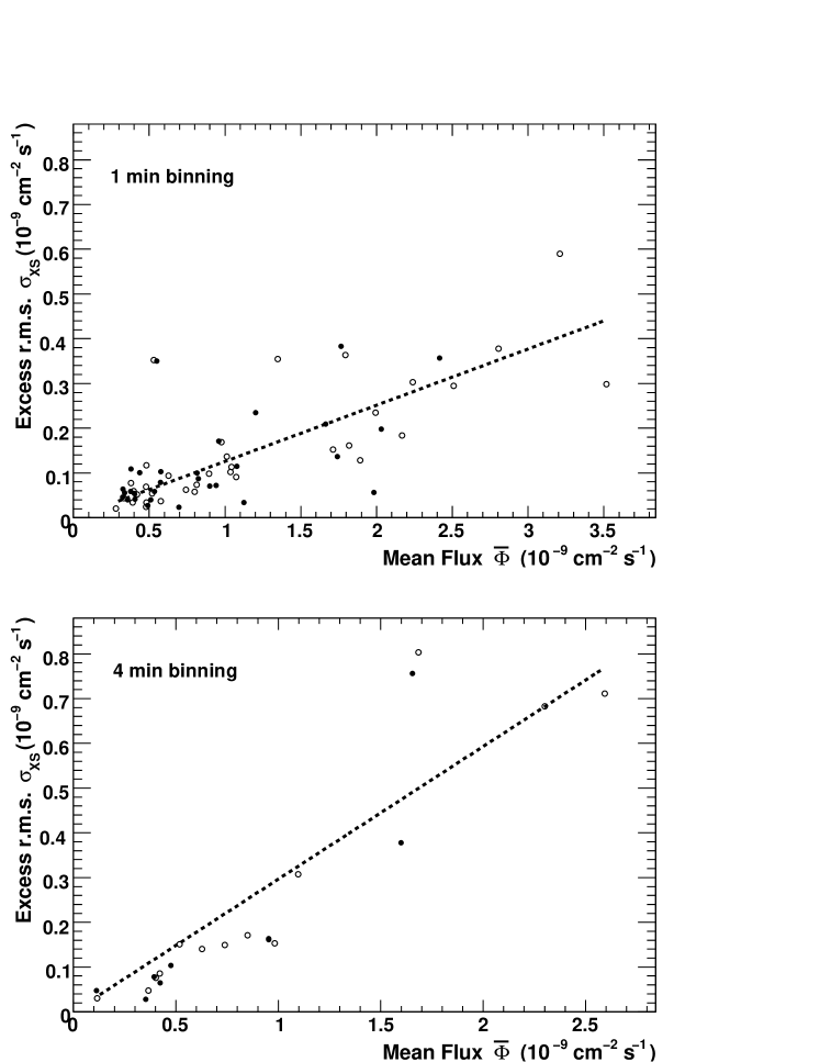
Having defined the shortest variability time scales, the nature of the process which generates the fluctuations is investigated, using another estimator: the excess r.m.s.. It is defined as the variance of a light curve (Eq. 5) after subtracting the measurement error:
| (6) |
Fig. 11 shows the correlation between the excess r.m.s. of the light curve and the flux, where the flux here considered are selected with an energy threshold of . The excess variance is estimated for 1- and 4-minute binned light curves, using 20 consecutive flux points which are at least at the significance level (81% of the 1 minute binned sample). The correlation factors are and for the 1 and 4 minute binning, excluding an absence of correlation at the and levels respectively, implying that fluctuations in the flux are probably proportional to the flux itself which is a characteristic of lognormal distributions (Aitchinson & Brown (1963)). This correlation has also been investigated extending the analysis to a statistically more significant data set including observations with a higher energy threshold in which the determination of the flux above requires an extrapolation (grey points in the top panel in Fig. 8). In this case the correlations found are compatible ( and for the 1 and 4 minute binning, respectively) and also exclude an absence of correlation with a higher significance ( and , respectively).
Such a correlation has already been observed for X-rays in the Seyfert class AGN (Edelson et al. (2002), Vaughan, Fabian & Nandra (2003), Vaughan et al. 2003, McHardy et al. (2004)) and in X-ray binaries (Uttley & McHardy (2001), Uttley (2004), Gleissner et al. (2004)), where it is
considered as evidence for an underlying stochastic multiplicative
process (Uttley, Mc Hardy & Vaughan (2005)), as opposed to an additive process. In additive processes, light
curves are considered as the sum of individual flares “shots”
contributing from several zones (multi-zone models) and the relevant
variable which has a Gaussian distribution (namely Gaussian
variable) is the flux.
For multiplicative (or cascade) models
the Gaussian variable is the logarithm of the flux. Hence, this first observation of
a strong r.m.s.-flux correlation in the VHE domain fully confirms the log-normality of the flux
distribution presented in Section 3.2.
.
6 Characterization of the lognormal process during the flaring period
This section investigates whether the variability of PKS 2155304 in the flaring period can be described by a random stationary process, where, as shown in Section 5.4, the Gaussian variable is the logarithm of the flux. In this case the variability can be characterized through its Power Spectral Density (PSD) (van der Klis (1997)) which indicates the density of variance as function of the frequency . The PSD is an intrinsic indicator of the variability, usually represented in large frequency intervals by power laws () and is often used to define different “states” of variable objects (see e.g., Paltani et al. (1997) and Zhang et al. 1999 for the PSD of PKS 2155304 in the optical and X-rays). The PSD of the light curve of one single night (MJD 53944) was given in Aharonian et al. (2007a) between and , and was found to be compatible with a red noise process (2) with times more power as in archival X-ray data (Zhang et al. 1999), but with a similar index. This study implicitely assumed the -ray flux to be the Gaussian variable. In the present paper, the PSD is determined using data from 4 consecutive nights (MJD 53944–53947) and assuming a lognormal process. Since direct Fourier analysis is not well adapted to light curves extending over multiple days and affected by uneven sampling and uneven flux errors, the PSD will be further determined on the basis of parametric estimation and simulations.
In the hypothesis where the process is stationary, i.e., the PSD is
time-independent, a power law shape of the PSD was assumed, as for
X-ray emitting blazars. The PSD was defined as depending on two paramenters and as follows:
, where is the variability spectral index and
denotes the “power” (i.e., the variance density) at a reference
frequency . This latter was conventionally chosen to be , where the two parameters
and are found to be decorrelated. Since a lognormal process is considered, is the density of variance of the
Gaussian variable . The
natural
logarithm of the flux is
conveniently used here, since its variance over a given frequency
interval666If is the variance of ,
. is close to the corresponding
value of , at least for small fluctuations. For a given
set of and , it is possible to simulate many long time
series, and to modify them according to experimental effects,
namely those of background events and of flux measurement errors.
Light curve segments are further extracted from this simulation,
with exactly the same time structure (observation and non-observation
intervals) and the same sampling rates as those of real data. The
distributions of several observables obtained from simulations for
different values of and will be compared to those determined
from observations, thus allowing these parameters to be determined
from a maximum-likelihood fit.
The simulation characteristics will be described in
Section 6.1. Sections 6.2, 6.3 and
6.4 will be devoted to the determination of and
by three methods, each of them based on an experimental result: the
excess r.m.s.–flux correlation, the Kolmogorov first-order structure
function (Rutman (1978); Simonetti et al. (1985)) and doubling-time measurements.
6.1 Simulation of realistic time-series
For practical reasons, simulated values of were calculated from Fourier series, thus with a discrete PSD. The fundamental frequency , which corresponds to an elementary bin in frequency, must be much lower than if is the duration of the observation. The ratio was chosen to be of the order of 100, in such a way that the influence of a finite value of on the average variance of a light curve of duration would be less than about 2%. Taking , this condition is fulfilled for the following studies. With this approximation, the simulated flux logarithms are given by:
| (7) |
where is chosen in such a way that is less
than the time interval between consecutive measurements (i.e., the
sampling interval). According to the definition of a Gaussian random
process, the phases are uniformly distributed between 0
and 2 and the Fourier coefficients are normally
distributed with mean 0 and variances given by
with .
From the long simulated time-series, light curve segments were
extracted with the same durations as the periods of continuous data
taking and with the same gaps between them. The simulated fluxes
were further smeared according to measurement errors, according to the
observing conditions (essentially zenith angle and background rate effects) in the
corresponding data set.
6.2 Characterization of the lognormal process by the excess r.m.s.–flux relation
For a fixed PSD, characterized by a set of parameters , 500 light curves were simulated, reproducing the observing conditions of the flaring period (MJD 53944–53947), according to the procedure explained in Section 6.1.
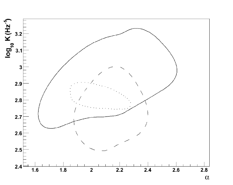
For each set of simulated light curves, segments of 20 minutes duration sampled every minute (and alternatively segments of 80 minutes duration sampled every 4 minutes) were extracted and, for each of them, the excess r.m.s. and the mean flux were calculated as explained in Section 5.4. For a large range of values of and , simulated light curves reproduce well the high level of correlation found in the measured light curves. On the other hand, the fractional variability and are essentially uncorrelated and will be used in the following. A likelihood function of and was obtained by comparing the simulated distributions of and to the experimental ones. An additional observable which is sensitive to and is the fraction of those light curve segments for which cannot be calculated because large measurement errors lead to a negative value for the excess variance. The comparison between the measured value of this fraction and those obtained from simulations is also taken into account in the likelihood function. The confidence contours for the two parameters and obtained from the maximum likelihood method are shown in Fig. 12 for both kinds of light curve segments. The two selected domains in the plane have a large overlap which restricts the values of to the interval (1.9, 2.4).
.
6.3 Characterization of the lognormal process by the structure function analysis
Another method for determining and is based on Kolmogorov structure functions (SF). For a signal , measured at pairs of times separated by a delay , , the first-order structure function is defined as (Simonetti et al. (1985)):
| (8) | |||
In the present analysis, represents the variable whose PSD is being estimated, namely . The structure function is a powerful tool for studying aperiodic signals (Rutman (1978), Simonetti et al. (1985)), such as the luminosity of blazars at various wavelengths. Compared to the direct Fourier analysis, the SF has the advantage of being less affected by “windowing effects” caused by large gaps between short observation periods in VHE observations. The first-order structure function is adapted to those PSDs whose variability spectral index is less than 3 Rutman (1978), which is the case here, according to the results of the preceding section.
Fig. 13 shows the first-order SF estimated for the flaring period (circles) for hr. At fixed , the distribution of expected for a given set of parameters is obtained from 500 simulated light curves. As an example, taking and , values of are found to lie at 68% confidence level within the shaded region in Fig. 13.
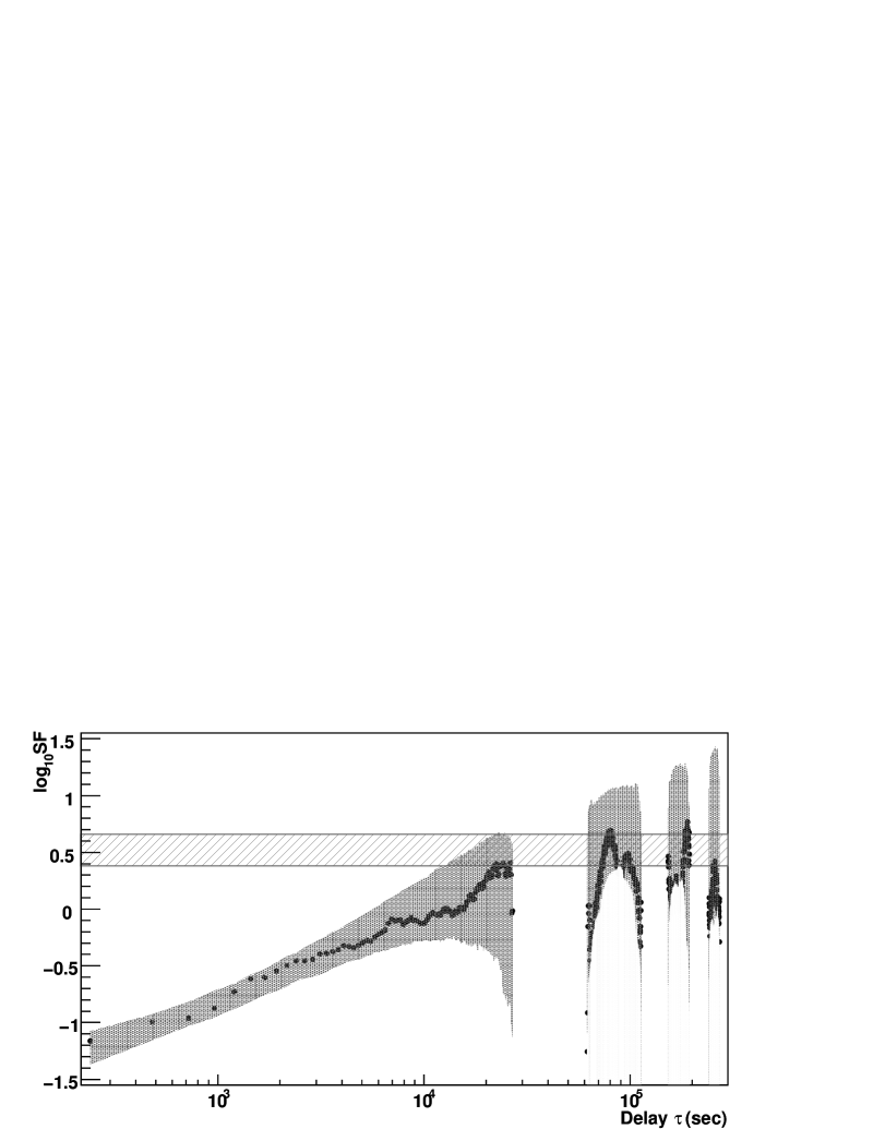
In the case of a power law PSD with index , the SF averaged over an ensemble of light curves is expected show a variation as (Kataoka et al. (2001)). However, this property does not take into account the effect of measurement errors, nor of the limited sensitivity of Cherenkov telescopes at lower fluxes. For the present study, it was preferable to use the distributions of obtained from realistic simulations including all experimental effects. Using such distributions expected for a given set of parameters , a likelihood function can be obtained from the experimental SF and further maximized with respect to these two parameters. Furthermore, the likelihood fit was restricted to values of lower than , for which the expected fluctuations are not too large and are well-controlled. The 95% confidence region in the plane thus obtained is indicated by the dotted line in Fig. 12. It is in very good agreement with those based on the excess r.m.s.–flux correlation and give the best values for and :
| (9) |
The variability index at VHE energies is found to be remarkably close to those measured in the X-ray domain on PKS 2155304, Mrk 421, and Mrk 501 (Kataoka et al. (2001)).
6.4 Characterization of the lognormal process by doubling times
Simulations were also used to investigate if the estimator can be used to constrain the values of and . However, for less than 2, no significant constraints on those parameters are obtained from the values of . For higher values of , doubling times only provide loose confidence intervals on which are compatible with the values reported above. This can be seen in Table 8, showing the 68% confidence intervals predicted for and for a lognormal process with =2 and , as obtained from simulation. Therefore, the variability of PKS 2155304 during the flaring period can be consistently described by the lognormal random process whose PSD is characterized by the parameters given by Eq. 9.
| MJD | Bin size | [min] | [min] |
|---|---|---|---|
| 53944 | 1 min | 0.93-1.85 | 1.60-2.60 |
| 53944 | 2 min | 3.01-4.28 | 4.52-6.40 |
| 53946 | 1 min | 1.8-2.3 | 1.96-2.41 |
| 53946 | 2 min | 5.3-9.1 | 6.6-12.1 |
7 Limits on characteristic time of PKS 2155304
In Section 5.2 the shortest variability time scale of PKS 2155304 using estimators like doubling times have been estimated. This corresponds to exploring the high frequency behaviour of the PSD. In this section the lower () frequency part of the PSD will be considered, aiming to set a limit on the timescale above which the PSD, characterized in Section 6, starts to steepen to . A break in the PSD is expected to avoid infrared divergences and the time at which this break occurs can be considered as a characteristic time, from which physical mechanisms occurring in AGN could be inferred.
| “Quiescent” regime | Flaring regime | |
|---|---|---|
| 0.304 0.040 | 1.78 0.27 | |
| 0.169 0.053 | 0.022 0.005 | |
| 0.135 0.067 | 1.758 0.273 |
Clearly the description of the source variability during the flaring period by a stationary lognormal random process is in good agreement with the flux distributions shown in Fig. 3. Considering the second Gaussian fit in the right panel of Fig. 3, the excess variance in the flaring regime reported in Table 9, although affected by a large error, is an estimator of the intrinsic variance of the stationary process. It has been demonstrated that represents the asymptotic value of the first-order structure function for large values of the delay (Simonetti et al. (1985)). On the other hand, as already mentioned, a PSD proportional to with cannot be extrapolated to arbitrary low frequencies; equivalently, the average structure function cannot rise as for arbitrarily long times. Therefore, by setting a 95% confidence interval on of from Table 9, it is possible to evaluate a confidence interval on a timescale above which the average value of the structure function cannot be described by a power law. Taking account of the uncertainties on and given by Eq. 9, leads to the 95% confidence interval for this characteristic time of the blazar in the flaring regime:
This is compatible with the behaviour of the experimental structure function at times s (Fig. 13), although the large fluctuations expected in this region do not allow a more accurate estimation. In the X-ray domain, characteristic times of the order of one day or less have been found for several blazars including PKS 2155304 (Kataoka et al. (2001)). The results presented here suggest a strong similarity between the PSDs for X-rays and VHE -rays during flaring periods.
8 Discussion and conclusions
This data set, which exhibits unique features and results, is the outcome of a long-term monitoring program and dedicated, dense, observations. One of the main results here is the evidence for a VHE -ray quiescent-state emission, where the variations in the flux are found to have a lognormal distribution. The existence of such a state was postulated by Stecker & Salamon (1996) in order to explain the extragalactic -ray background at 0.03– detected by EGRET (Fichtel (1996); Sreekumar et al. (1998)) as coming from quiescent-state unresolved blazars. Such a background has not yet been detected in the VHE range, as it is technically difficult with the atmospheric Cherenkov technique to find an isotropic extragalactic emission and even more to distinguish it from the cosmic-ray electron flux (Aharonian et al. 2008b ). In addition, the EBL attenuation limits the distance from which TeV -rays can propagate to (Aharonian et al. 2007b ). As pointed out by Cheng, Zhang and Zhang (2000), emission mechanisms might be simpler to understand during quiescent states in blazars, and they are also the most likely state to be found observationally. In the X-ray band, the existence of a steady underlying emission has also been invoked for two other VHE emitting blazars (Mrk 421, Fossati et al. (2000), and 1ES 1959+650, Giebels et al. (2002)). Being able to separate, and detect, flaring and nonflaring states in VHE -rays is hence important for such studies.
The observation of the spectacular outbursts of PKS 2155304 in July 2006 represents one the most extreme examples of AGN variability in the TeV domain, and allows spectral and timing properties to be probed over two orders of magnitude in flux.
Whereas for the flaring states with fluxes above a few a clear hardening of the spectrum with increasing flux is observed, familiar also from the blazars Mrk 421 and Mrk 501, for the quiescent state in contrast an indication of a softening is noted. If confirmed, this is a new and intruiging observation in the VHE regime of blazars. The blazar PKS 0208512 (of the FSRQ class) also shows such initial softening and subsequent hardening with flux in the MeV range, but no general trend could be found for -ray blazars (Nandikotkur et al. (2007)). In the framework of synchrotron self-Compton scenarios, VHE spectral softening with increasing flux can be associated with, for example, an increase in magnetic field intensity, emission region size, or the power law index of the underlying electron distribution, keeping all other parameters constant. A spectral hardening can equally be obtained by increasing the maximal Lorentz factor of the electron distribution or the Doppler factor (see e.g. Fig. 11.7 in Kataoka (1999)). A better understanding of the mechanisms at play would require multi-wavelength observations of similar time span and sampling density as the data set presented here.
It is shown that the variability time scale of a few minutes are only upper limits for the intrinsic lowest characteristic time scale. Doppler factors of of the emission region are derived by Aharonian et al. (2007a) using the black hole (BH) Schwarzschild radius light crossing time as a limit, while Begelman et al. (2008) argue that such fast time scales cannot be linked to the size of the BH and must occur in regions of smaller scales, such as “needles” of matter moving faster than average within a larger jet (Ghisellini & Tavecchio (2008)), small components in the jet dominating at TeV energies (Katarzyński et al. (2008)), or jet “stratification” (Boutelier, Henri & Petrucci (2008)). Levinson (2007) attributes the variability to dissipation in the jet coming from radiative deceleration of shells with high Lorentz factors.
The flaring period allowed the study of light curves in separated energy bands and the derivation of a power law dependence of with the energy (). This dependence is comparable to that reported in Giebels et al. (2007), Lichti et al. (2008), Maraschi et al. (2002), where between the optical and X-ray energy bands was found for Mrk 421 and PKS 2155304, respectively. An increase with the energy of the flux variability has been found for Mrk 501 (Albert et al. 2007) in VHE -rays on timescales comparable to those observed here.
The flaring period showed for the first time that the intrinsic variability of PKS 2155304 increases with the flux, which can itself be described by a lognormal process, indicating that the aperiodic variability of PKS 2155304 could be produced by a multiplicative process. The flux in the “quiescent regime”, which is on average 50 times lower than in the flaring period and has a 3 times lower , also follows a lognormal distribution, suggesting similarities between these two regimes.
It has been possible to characterize a power spectral density of the flaring period in the frequency range –, resulting in a power law of index valid for frequencies down to . The description of the rapid variability of a TeV blazar as a random stationary process must be taken into account by time-dependent blazar models. For PKS 2155304 the evidence of this log-normality has been found very recently in X-rays (Giebels & Degrange (2009)) and as previously mentioned, X-ray binaries and Seyfert galaxies also show lognormal variability, which is thought to originate from the accretion disk (McHardy et al. (2004); Lyubarskii et al. (1997); Arévalo and Uttley (2006)), suggesting a connection between the disk and the jet. This variability behaviour should therefore be searched for in existing blazar light curves, independently of the observed wavelength.
Acknowledgements
The support of the Namibian authorities and of the University of Namibia in facilitating the construction and operation of H.E.S.S. is gratefully acknowledged, as is the support by the German Ministry for Education and Research (BMBF), the Max Planck Society, the French Ministry for Research, the CNRS-IN2P3 and the Astroparticle Interdisciplinary Programme of the CNRS, the U.K. Science and Technology Facilities Council (STFC), the IPNP of the Charles University, the Polish Ministry of Science and Higher Education, the South African Department of Science and Technology and National Research Foundation, and by the University of Namibia. We appreciate the excellent work of the technical support staff in Berlin, Durham, Hamburg, Heidelberg, Palaiseau, Paris, Saclay, and in Namibia in the construction and operation of the equipment.
References
- Aharonian et al. (2002) Aharonian, F. et al. (HEGRA. Collaboration) 2002, A&A, 393, 89
- (2) Aharonian, F. et al. (H.E.S.S. Collaboration) 2005a, A&A, 437, 95
- (3) Aharonian, F. et al. (H.E.S.S. Collaboration) 2005b, A&A, 430, 865
- (4) Aharonian, F. et al. (H.E.S.S. Collaboration) 2005c, A&A, 442, 895
- (5) Aharonian, F. et al. (H.E.S.S. Collaboration) 2006, A&A, 457, 899
- (6) Aharonian, F. et al. (H.E.S.S. Collaboration) 2007a, ApJ, 664, L71
- (7) Aharonian, F. et al. (H.E.S.S. Collaboration) 2007b, A&A, 475, L9
- (8) Aharonian, F. et al. (H.E.S.S. Collaboration) 2008a, Phys. Rev. Lett, 101, 170402
- (9) Aharonian, F. et al. (H.E.S.S. Collaboration) 2008b, Phys. Rev. Lett, 101, 261104
- (10) Aharonian, F. et al. (H.E.S.S. Collaboration) 2009, A&A, 502, 749
- Aitchinson & Brown (1963) Aitchinson, J., Brown, J.A.C. 1963,“The Lognormal Distribution (Cambridge University Press, Cambridge)”
- (12) Albert, J. et al. (MAGIC Collaboration) 2007, ApJ, 669, 862
- Arévalo and Uttley (2006) Arévalo, P. &Uttley, P. 2006, MNRAS, 367, 801
- Begelman et al. (2008) Begelman, M.C., Fabian, A.C. & Rees, M.J. 2008, MNRAS, 384, L19
- Boutelier, Henri & Petrucci (2008) Boutelier, T., Henri, G., & Petrucci, P. O. 2008, MNRAS, 390, 73
- Chadwick et al. (1999) Chadwick, P. et al. 1999, ApJ, 513, 161
- Cheng, Zhang and Zhang (2000) Cheng, K. S., Zhang, X., and Zhang, L. 2000, ApJ, 537, 80 al. 1999, ApJ, 521, 522
- Djannati-Ataï et al. (1999) Djannati-Ataï, A. et al. 1999, A&A, 350, 17
- Edelson et al. (2002) Edelson, R. et al. 2002, ApJ, 568, 610
- Edelson & Krolik (1988) Edelson, R.A. & Krolik, J. H. 1988, ApJ, 333, 646
- Fichtel (1996) Fichtel, C. 1996, A&AS, 120, 23
- Fossati et al. (2000) Fossati, G. et al. 2000, ApJ, 541, 153
- Ghisellini & Tavecchio (2008) Ghisellini, G. & Tavecchio, F. 2008, MNRAS, 386, 28
- Giebels et al. (2002) Giebels, B. et al. 2002, ApJ, 571, 763
- Giebels et al. (2005) Giebels, B. et al. (H.E.S.S. Collaboration) 2005, Proc. of the Annual meeting of the French Society of Astronomy and Astrophysics (Strasbourg), 527
- (26) Giebels, B., Dubus, G., & Khelifi, B. 2007, A&A, 462, 29
- Giebels & Degrange (2009) Giebels, B. & Degrange, B. 2009, A&A, 503, 797
- Gleissner et al. (2004) Gleissner, T. et al. 2004, A&A, 414, 1091
- Katarzyński et al. (2008) Katarzyński, K. et al. 2008, MNRAS, 390, 371
- Kataoka (1999) Kataoka, J. 1999, “X-ray Study of Rapid Variability in TeV Blazars and the Implications on Particle Acceleration in Jets”, ISAS RN 710
- Kataoka et al. (2001) Kataoka, J. et al. 2001, ApJ , 560, 659
- Lemoine-Goumard, Degrange & Tluczykont (2006) Lemoine-Goumard, M., Degrange, B., & Tluczykont, M. 2006, Astropart. Phys., 25, 195
- Levinson (2007) Levinson, A. 2007, ApJ ,671, L29
- (34) Lichti, G., et al. 2008, A&A, 486, 721
- Lyubarskii et al. (1997) Lyubarskii, Y.E. 1997, MNRAS, 292, 679
- (36) Maraschi, L. et al. 2002, Proceedings of the Symposium “New Visions of the X-ray Universe in the XMM-Newton and Chandra Era”, ESTEC 2001, [arXiv:0202418v1]
- McHardy et al. (2004) McHardy, I.M. et al. 2004, MNRAS, 348, 783
- Nandikotkur et al. (2007) Nandikotkur, G. et al. 2007, ApJ, 657, 706
- Nandra et al. (1997) Nandra, K. et al. 1997, ApJ, 476, 70
- Paltani et al. (1997) Paltani, S. et al. 1997, A&A, 327, 539
- Piron et al. (2001) Piron, F. et al. 2001, A&A, 374, 895
- Poutanen & Stern (2008) Poutanen, J. & Stern, B.E. 2008, Int. Journal of Modern Physics, 17, 1619
- Rutman (1978) Rutman, J., Proc. IEEE 1978, 66, 1048.
- Simonetti et al. (1985) Simonetti, J.H., Cordes, J.M. Heeschen D.S. 1985, ApJ, 296, 46
- Sreekumar et al. (1998) Sreekumar, P. et al. 1998, ApJ, 494, 523
- Stecker & Salamon (1996) Stecker, F. W. & Salamon, M. H. 1996, ApJ, 464, 600
- Stern (2003) Stern, B.E. 2003, MNRAS, 345, 590
- Stern & Poutanen (2006) Stern, B.E. & Poutanen, J. 2006, MNRAS, 372, 1217
- Spada et al. (2001) Spada, M. et al., 2001, MNRAS 325, 1559
- Takahashi et al. (2000) Takahashi,T., et al. 2000, ApJ, 542, L105
- Uttley & McHardy (2001) Uttley, P. & Mc Hardy, I.M. 2001, MNRAS, 323, L26
- Uttley (2004) Uttley, P. 2004, MNRAS, 347, L61
- Uttley, Mc Hardy & Vaughan (2005) Uttley, P., Mc Hardy, I.M., & Vaughan, S. 2005, MNRAS, 359, 345
- van der Klis (1997) van der Klis, M. 1997, Proceeding of the conference ”Statistical Challenges in Modern Astronomy II”, Pennsylvania State University, Ed. Springer-Verlag Berlin, 321
- Vaughan, Fabian & Nandra (2003) Vaughan, S., Fabian, A.C., & Nandra, K. 2003, MNRAS, 339, 1237
- (56) Vaughan, S. et al. 2003, MNRAS, 345, 1271
- White & Peterson (1984) White, R.J. & Peterson, B.M. 1994, PASP, 106, 879
- (58) Zhang, Y.H. et al. 1999, ApJ, 527, 719
Appendix A Observations summary
The journal of observations for the 2005-2007 is presented in Table 10.
| MJD | Excess | ||||||
|---|---|---|---|---|---|---|---|
| 53618 | 16.9 | 0.87 | 860 | 3,202 | 219.6 | 7.5 | 8.0 |
| 53637 | 16.6 | 1.09 | 788 | 2,673 | 253.4 | 9.2 | 8.8 |
| 53638 | 14.7 | 2.18 | 1,694 | 6,029 | 488.2 | 12.0 | 8.1 |
| 53665 | 22.6 | 0.87 | 618 | 2,487 | 120.6 | 4.7 | 5.1 |
| 53666 | 26.3 | 1.31 | 857 | 3,406 | 175.8 | 5.9 | 5.1 |
| 53668 | 23.3 | 1.30 | 926 | 3,793 | 167.4 | 5.3 | 4.7 |
| 53669 | 19.6 | 0.86 | 1,027 | 2,939 | 439.2 | 14.7 | 15.8 |
| 53705 | 55.6 | 0.88 | 512 | 2,542 | 3.6 | 0.1 | 0.2 |
| 53916 | 13.7 | 0.88 | 993 | 3,317 | 329.6 | 10.7 | 11.5 |
| 53917 | 11.8 | 0.88 | 933 | 3,163 | 300.4 | 10.1 | 10.7 |
| 53918 | 10.2 | 1.32 | 1,491 | 4,596 | 571.8 | 15.5 | 13.5 |
| 53919 | 10.9 | 1.32 | 1,477 | 4,638 | 549.4 | 14.9 | 13.0 |
| 53941 | 14.4 | 1.31 | 2,445 | 4,844 | 1,476.2 | 35.0 | 30.6 |
| 53942 | 13.7 | 1.76 | 2,453 | 5,766 | 1,299.8 | 29.5 | 22.3 |
| 53943 | 9.8 | 1.33 | 1,142 | 3,627 | 416.6 | 12.8 | 11.1 |
| 53944 | 13.2 | 1.33 | 12,762 | 3,563 | 12,049.4 | 172.9 | 149.7 |
| 53945 | 23.9 | 5.23 | 8,037 | 16,352 | 4766.6 | 62.0 | 27.1 |
| 53946 | 27.7 | 6.61 | 35,874 | 19,881 | 31,897.8 | 251.3 | 97.7 |
| 53947 | 25.1 | 5.89 | 17,158 | 17,006 | 13,756.8 | 142.6 | 58.8 |
| 53948 | 27.7 | 2.75 | 5,366 | 7,957 | 3,774.6 | 64.6 | 38.9 |
| 53950 | 26.6 | 3.51 | 5,108 | 11,955 | 2,717.0 | 42.8 | 22.9 |
| 53951 | 28.4 | 2.51 | 3,275 | 8,421 | 1,590.8 | 30.6 | 19.3 |
| 53952 | 35.8 | 1.76 | 1,786 | 5,395 | 707.0 | 17.7 | 13.3 |
| 53953 | 44.1 | 0.89 | 670 | 2,285 | 213.0 | 8.4 | 8.9 |
| 53962 | 27.6 | 0.89 | 534 | 2,088 | 116.4 | 4.9 | 5.3 |
| 53963 | 19.4 | 1.75 | 1,613 | 6,145 | 384.0 | 9.5 | 7.1 |
| 53964 | 10.3 | 1.49 | 1,057 | 4,146 | 227.8 | 6.9 | 5.6 |
| 53965 | 15.7 | 1.57 | 1,584 | 5,662 | 451.6 | 11.4 | 9.1 |
| 53966 | 18.6 | 0.88 | 719 | 2,844 | 150.2 | 5.5 | 5.8 |
| 53967 | 24.3 | 0.86 | 481 | 1,801 | 120.8 | 5.5 | 5.9 |
| 53968 | 19.1 | 0.86 | 479 | 1,974 | 84.2 | 3.7 | 4.0 |
| 53969 | 21.2 | 1.29 | 1,738 | 4,368 | 864.4 | 23.0 | 20.2 |
| 53970 | 20.9 | 0.88 | 690 | 2,759 | 138.2 | 5.1 | 5.5 |
| 53971 | 19.8 | 1.32 | 1,449 | 4,313 | 586.4 | 16.3 | 14.2 |
| 53972 | 16.5 | 1.30 | 683 | 2,499 | 183.2 | 7.0 | 6.1 |
| 53973 | 14.5 | 1.32 | 1,157 | 4,311 | 294.8 | 8.6 | 7.5 |
| 53974 | 16.2 | 1.76 | 1,504 | 5,925 | 319.0 | 8.1 | 6.1 |
| 53975 | 15.8 | 0.88 | 804 | 3,059 | 192.2 | 6.7 | 7.2 |
| 53976 | 13.8 | 0.89 | 727 | 2,544 | 218.2 | 8.2 | 8.7 |
| 53977 | 12.0 | 0.88 | 832 | 2,745 | 283.0 | 10.1 | 10.8 |
| 53978 | 13.3 | 0.89 | 687 | 2,317 | 223.6 | 8.7 | 9.3 |
| 53995 | 21.4 | 1.75 | 1,712 | 5,989 | 514.2 | 12.6 | 9.5 |
| 53996 | 25.3 | 1.33 | 680 | 2,834 | 113.2 | 4.2 | 3.6 |
| 53997 | 26.3 | 1.32 | 1,113 | 4,382 | 236.6 | 7.0 | 6.1 |
| 53998 | 26.1 | 1.32 | 1,247 | 4,082 | 430.6 | 12.6 | 11.0 |
| 53999 | 21.4 | 1.32 | 1,107 | 4,262 | 254.6 | 7.5 | 6.6 |
| 54264 | 8.5 | 0.13 | 109 | 449 | 19.2 | 1.8 | 5.0 |
| 54265 | 8.5 | 1.05 | 920 | 3,513 | 217.4 | 7.1 | 6.9 |
| 54266 | 9.3 | 1.39 | 1,129 | 4,553 | 218.4 | 6.3 | 5.4 |
| 54267 | 9.2 | 1.32 | 1,095 | 4,176 | 259.8 | 7.8 | 6.7 |
| 54268 | 10.2 | 0.32 | 261 | 1,040 | 53.0 | 3.2 | 5.6 |
| 54269 | 9.1 | 0.89 | 908 | 2,491 | 409.8 | 14.7 | 15.6 |
| 54270 | 10.8 | 0.44 | 565 | 1,266 | 311.8 | 14.9 | 22.4 |
| 54271 | 7.6 | 0.36 | 308 | 983 | 111.4 | 6.6 | 11.0 |
| 54294 | 7.7 | 0.44 | 447 | 1,337 | 179.6 | 9.0 | 13.5 |
| 54296 | 7.2 | 0.44 | 350 | 1,289 | 92.2 | 4.9 | 7.4 |
| 54297 | 9.8 | 0.44 | 344 | 1,265 | 91.0 | 4.9 | 7.4 |
| 54299 | 7.6 | 0.44 | 347 | 1,232 | 100.6 | 5.5 | 8.2 |
| 54300 | 7.3 | 0.44 | 343 | 1,245 | 94.0 | 5.1 | 7.6 |
| 54302 | 7.7 | 0.44 | 358 | 1,234 | 111.2 | 6.0 | 9.0 |
| 54304 | 7.9 | 0.88 | 680 | 2,765 | 127.0 | 4.7 | 5.0 |
| 54319 | 8.9 | 0.88 | 692 | 2,650 | 162.0 | 6.1 | 6.5 |
| 54320 | 8.0 | 0.89 | 553 | 2,199 | 113.2 | 4.7 | 5.0 |
| 54329 | 11.7 | 0.44 | 297 | 1,258 | 45.4 | 2.5 | 3.8 |
| 54332 | 7.0 | 0.16 | 100 | 391 | 21.8 | 2.1 | 5.3 |
| 54375 | 9.4 | 1.27 | 811 | 3,124 | 186.2 | 6.4 | 5.7 |
| 54376 | 7.9 | 0.68 | 395 | 1,605 | 74.0 | 3.6 | 4.4 |
Appendix B Spectral variability
The numerical information associated with Fig. 7 is given in Tables 11 (left panel, grey points), 12 (left panel, black points) and 13 (right panel). In addition, numerical information associated with Fig. 8 is given in Table 14.
| Index | |
|---|---|
| Index | |
|---|---|