Vibrational Spectrum of Granular Packings With Random Matrices
Abstract
The vibrational spectrum of granular packings can be used as a signature of the jamming transition, with the density of states at zero frequency becoming non-zero at the transition. It has been proposed previously that the vibrational spectrum of granular packings can be approximately obtained from random matrix theory. Here we show that although the density of states predicted by random matrix theory does not agree with certain aspects of dynamical numerical simulations, the correlations of the density of states, which—in contrast to the density of states—are expected to be universal, do show good agreement between dynamical numerical simulations of bead packs near the jamming point and the analytic predictions of the Laguerre orthogonal ensemble of random matrices. At the same time, there is clear disagreement with the Gaussian orthogonal ensemble. These findings establish that the Laguerre ensemble correctly reproduces the universal statistical properties of jammed granular matter and exclude the Gaussian orthogonal ensemble. We also present a random lattice model which is a physically motivated variant of the random matrix ensemble. Numerical calculations reveal that this model reproduces the known features of the vibrational density of states of granular matter, while also retaining the correlation structure seen in the Laguerre random matrix theory. We propose that the random lattice model can therefore be applied the understand not only the spectrum but more general properties of the vibration of bead packs including the spatial structure of modes both at the jamming point and far from it.
I Introduction
Granular materials are a class of systems which are out of equilibrium and not easy to understand within the framework of standard statistical mechanics. For static assemblies, the distribution of forces Coppersmith and the continuum limit Cates are difficult to obtain. This is because interparticle contacts are very stiff: a slight compression of two particles that are contact, by an amount that is much less than the interparticle separation, gives rise to large forces. Added complications are caused by the fact that, for noncohesive granular matter, two particles in contact repel each other when they are compressed, but do not attract each other when they are moved away from each other and the contact is broken; that the repulsive force between particles is not a linear function of their compression when the compression is small; MvHreview and that there are frictional forces between particles, Bi resulting in history dependent forces. The dynamic properties of granular matter are difficult to understand because interparticle collisions are strongly inelastic. If a high density of particles builds up in a region because of random fluctuations, the collision rate and therefore the rate of energy loss increases in the region. This can trap particles in the region, causing the density fluctuations to grow. Goldhirsch Experimentally, one observes distinctive phenomena such as force chains and stability against mechanical collapse in very sparse static packings, non-Maxwellian velocity distributions vanNoije ; Rouyer ; Reis and inelastic collapse in dilute granular gases, McNamara ; Hopkins and shear thinning and shear thickening in the intermediate regime. Brown
The tendency of flowing granular matter to get ‘jammed’ and stop flowing at low densities is a practical problem that limits the flow rate in the industrial use of granular materials. LiuNagelCRCBook Remarkably,the transition from a flowing to a jammed state in granular matter, structural glasses, and foams and colloids, can be studied with a unified approach. LiuNagel1998 When the transition occurs at zero temperature and zero shear stress as the density is varied, the transition point is called “Point J”, OHern and is characterized by diverging length scales Wyart ; Ellenbroek suggestive of a second order phase transition. At the same time, other properties of the system change discontinuously at Point J, OHern as one would expect at a first order phase transition.
The density of states for vibrational modes in a granular system is one of the properties that has a signature of the transition at Point J. A jammed granular system has mechanical rigidity. Even though the force between two particles is a nonlinear function of the compression between them, the small deviations from the jammed state (which already has non-zero compression) can be analyzed using a linear model, resulting in normal modes. Extensive numerical simulations OHern on systems at zero temperature and zero shear stress show that the density of states as a function of approaches zero linearly as if the particle density is greater than the critical density. As the particle density is reduced, the slope of at the origin becomes steeper, until at Point J,
In the linearized analyis of vibrational modes, the system can be treated as a network of random springs, with the number of springs decreasing as Point J is approached. It is natural to analyze the problem using random matrices, and see how the resultant density of states evolves near the transition. This has been done, beltukov and yields a broad peak in the density of states that reaches as the transition is approached. However, the model also predicts a gap in the density of states near above the transition, which does not match the numerical results. There are a few other qualitative discrepancies.
Although it is encouraging that some features of the random matrix density of states matches from numerical simulations, it is well known that the overall density of states predicted by random matrix theory often differs from what is observed in systems to which the theory applies, because of non-universal effects mehta . Instead, the correlations in the density of states and the distribution of level spacings is a more reliable indicator of the validity of the random matrix approach mehta .
In this paper we therefore turn to the correlations in the density of states predicted by random matrix theory. We argue that the Laguerre orthogonal ensemble rather than the Gaussian orthogonal ensemble (GOE) is the appropriate random matrix model for granular bead packs. The correlation function for the Laguerre ensemble differs from that for the GOE near the low-frequency edge of the allowed range of nagao . By comparing the correlations in the numerically computed vibrational spectrum of granular bead packs near the jamming transition to the predictions of the Laguerre ensemble and the GOE we are able to demonstrate good agreement with the former and to exclude the latter.
The distribution of consecutive level spacings is also a universal feature of the spectrum that should be described by random matrix theory. We find that the level spacing distribution predicted by the Laguerre ensemble is very close to the GOE result both near the zero frequency edge and at high frequency. The spectra calculated for granular bead packs in dynamical simulations are found to agree with this distribution. This finding further validates the random matrix approach but it does not help discriminate between the Laguerre ensemble and the GOE. The agreement of the level spacing distribution with the GOE result has been observed earlier, Silbert ; Nelson but without reference to the Laguerre ensemble.
We also construct a random lattice model, which is a physically motivated variant of the random matrix ensemble. Although it is not possible to calculate the properties of this model analytically, numerical results reveal that all the qualitative features of are reproduced. At the same time, the correlation functions and the level spacing distribution seen in the idealized random matrix theory are not significantly changed.
The rest of the paper is organized as follows. In section II we summarize the random matrix approach to the problem and the results for the density of states. In Section III we compare the autocorrelation function for the density of states and the level spacing distribution for the Laguerre ensemble and the GOE to the vibrational spectra for granular packs near point J, obtained from dynamical numerical simulations. In Section IV we introduce the random lattice model and show that it reproduces both universal and non-universal features of vibrational spectrum of granular packs. In Appendix A we present an analysis of the level spacing distribution for the Laguerre ensemble and in Appendix B some technical details regarding the autocorrelation.
II Laguerre ensembles
We follow the approach of Ref. beltukov here. Within linear response, if the particles in the granular assembly are displaced slightly from their resting positions, their accelerations are of the form where is a component column vector and is a matrix. The crucial observation lubensky ; calladine is that the connection between accelerations and displacements is a two-step process. Within linear response, each contact between a pair of particles can be represented as a spring that has been precompressed by some amount. Thus one has a network of springs, with various spring constants. When a particle is displaced, it stretches (or compresses) each spring that it is connected to, by an amount that is equal to the component of its displacement along that spring. The spring exerts a restoring force that is proportional to this stretching; the spring constant can be different for each spring. Thus we have
| (1) |
where if the ’th spring is connected to the ’th particle, with being the angle between the displacement and the direction of the spring, and otherwise. The restoring force on each particle is the sum of the forces from all the springs it is connected to, so that
| (2) |
i.e.
| (3) |
Defining this is equivalent to
| (4) |
Even though we have presented the argument as if the displacement of each particle is one scalar variable, it is easy to extend this to particles in a -dimensional system, with displacement variables for particles. We have implicitly assumed that the particles are frictionless spheres, so that torque balance is trivially satisfied.
The matrix is a rectangular matrix, since the number of springs is greater than As one approaches Point J, the number of contact forces decreases, being equal to at the transition.
In the random matrix approach to this problem, we assume that all the entries in the matrix are independent Gaussian random variables, drawn from a distribution with zero mean and (with a suitable rescaling) unit variance. This is the Laguerre random matrix ensemble. It can be shown Forrester that the reduced probability density for the eigenvalues of is of the form
| (5) |
where the matrix is a dimensional matrix, i.e. there are inter-particle contacts in the system, and without loss of generality we have chosen all the ’s to be greater than zero.
Rewriting the probability density in terms of we have
| (6) |
where If is a saddle-point expansion yields
| (7) |
wherever Here is the density of eigenvalues, normalized to and the denotes the principal value of the integral. Symmetrizing by defining the function
| (8) |
of the complex variable is analytic everywhere except that it has branch cuts on the real line over intervals where where it is equal to
| (9) |
Furthermore, is finite, and because the symmetrized extension of integrates to 2. This has the solution
| (10) |
with
| (11) |
The density of states is then
| (12) |
where we have removed the extension of to so that The density of states has the same form, but with and rescaled, which is not significant since Eq.(5) was already obtained after rescaling.
When there is a broad peak in with a gap in the spectrum near The peak is not symmetric, falling off much more sharply on the small side than on the large side. In the middle, the peak slopes downwards as is increased. As is reduced, the gap shrinks while the width of the peak remains constant. When which matches the Wigner semicircle law for the Gaussian orthogonal ensemble, and
One can compare these analytical predictions with numerical results. Simulations of two-dimensional frictionless soft spheres are performed, allowing the spheres to equilibrate from an initial random configuration Corey . As with the analytical prediction, there is a broad peak, that falls off more sharply at small than at large The density of states except at the transition. However, the numerical data does not show the gap in the spectrum near predicted by random matrix theory. The numerical data also has a pronounced boson peak at a non-zero value of and a cusp in at the origin at the transition. None of these is consistent with the prediction from random matrix theory. We return to this point in Section IV.
III Correlations
In this section we subject the predictions of the random matrix model to more stringent and appropriate tests. We have seen in the previous section the mean density of states of the random matrix model does not exactly match the density of states of the dynamical numerical simulation of a granular pack. However that is not the appropriate test of a random matrix model. In all of its successful applications, what random matrix theory is able to predict correctly is not the mean density of states, but rather statistical features like the density of states correlation and the level spacing distribution, that are computed after the spectrum has been smoothed by a procedure called unfolding (explained below) that makes the mean density of states uniform.
Theoretically one can understand this as follows. It can be shown brezin that, for an ensemble of random matrices, the mean density of states can be changed at will by varying the assumed distribution of the matrix elements, but that the correlations of the unfolded spectrum retain a universal form that depends only on the symmetries of the ensemble considered (such as whether the matrices are real or complex or quaternion real). From this point of view the mean density of states we obtained in the previous section is simply an artifact of the Gaussian distribution we chose for our random matrix elements, but the unfolded density of states correlations and the level spacing distribution are universal and should match the numerical data for jammed granular matter if the model is applicable.
The key feature of the random matrix spectrum is that it is rigid (i.e. highly correlated). The rigidity of the spectrum is revealed at small energy scales by the distribution of consecutive level spacings. The longer range rigidity can be demonstrated by the autocorrelation of the density of states or by specific statistical measures such as the number statistic and the spectral rigidity mehta .
Insight into the strong correlations between the eigenvalues implied by the Laguerre ensemble distribution Eq.(5) is provided by the following plasma analogy. We focus on the case since we are interested in the spectrum for point J. If we rewrite rewrite the factor in Eq.(5) as and the factor as , we can interpret Eq. (5) as the partition function of a classical plasma of N particles located on the positive axis at the locations with logarithmic interactions between the particles as well as logarithmic interactions between each particle and image particles at locations . In the plasma analogy the particles are also confined near the origin by a quadratic potential and are constrained to remain on the positive axis by a hard wall at the origin.
We turn now to the distribution of spacings between consecutive levels. Intuitively one might expect that the spacing between consecutive levels at low frequency would be different from that between two levels at high frequency. This is because, in terms of the plasma analogy, in the first instance the two interacting levels are near the hard wall, whereas in the latter instance they are deep in the interior of the plasma. However, we show in Appendix A that the consecutive level spacing distribution is not noticeably different for high and low frequencies, and neither of these is noticeably different from the distribution for the GOE.
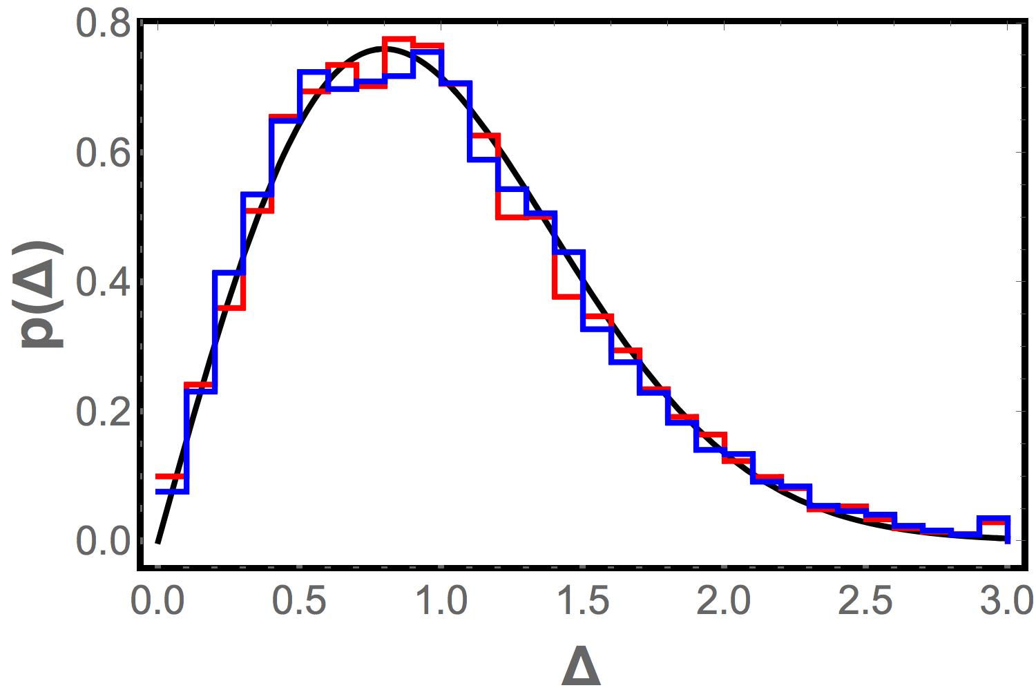
In Fig. 1 we compare the predictions of the Laguerre model to the numerically computed jammed granular spectrum. The red histogram bins the eleven consecutive level spacings between the frequencies through for each realization; each spacing is normalized by where the average is taken over the one thousand realizations of the jammed granular pack. The blue histogram is the same but for the eleven level spacings between the frequencies through . The two distributions are seen to be indistinguishable and to be in good agreement with the approximate analytic formula for the Laguerre ensemble (solid black curve) which is itself indistinguishable from the prediction of the GOE at the resolution of the figure.
Fig. 1 shows that the numerical level spacing distribution is consistent with the prediction of the Laguerre random matrix model and hence is a validation of that model. However, the level spacing distribution is not able to distinguish between the Laguerre model and the GOE, and is therefore a less sharp test of the Laguerre model than the density of states autocorrelation to which we now turn.
In order to calculate these correlations it is convenient to rewrite the distribution in Eq. (5) for the case in the form
| (13) |
where . The one-point and two-point correlation functions are defined as
| (14) |
and
| (15) |
The plasma analogy shows that calculation of the correlation functions in Eq. (14) and Eq. (15) is a formidable problem in classical statistical mechanics. Nonetheless it has been exactly done by Nagao and Slevin nagao by rewriting Eq. (13) in the form of a quaternion determinant and performing the integrals by a generalization of a theorem of Dyson dyson on integration over quaternion determinants. Before we give those results we first describe the unfolding procedure.
is evidently the density of states, and we now define
| (16) |
where is the cumulative density of states. The unfolded two point correlation function is then defined as
| (17) |
It is easy to see that if is similarly defined then showing that after unfolding the density of states is uniform with a mean level spacing of unity. The exact expression for is rather lengthy and is relegated to Appendix B.
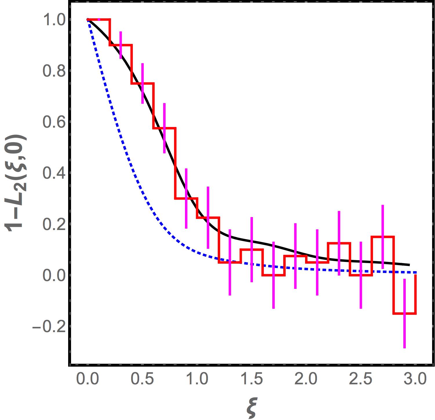
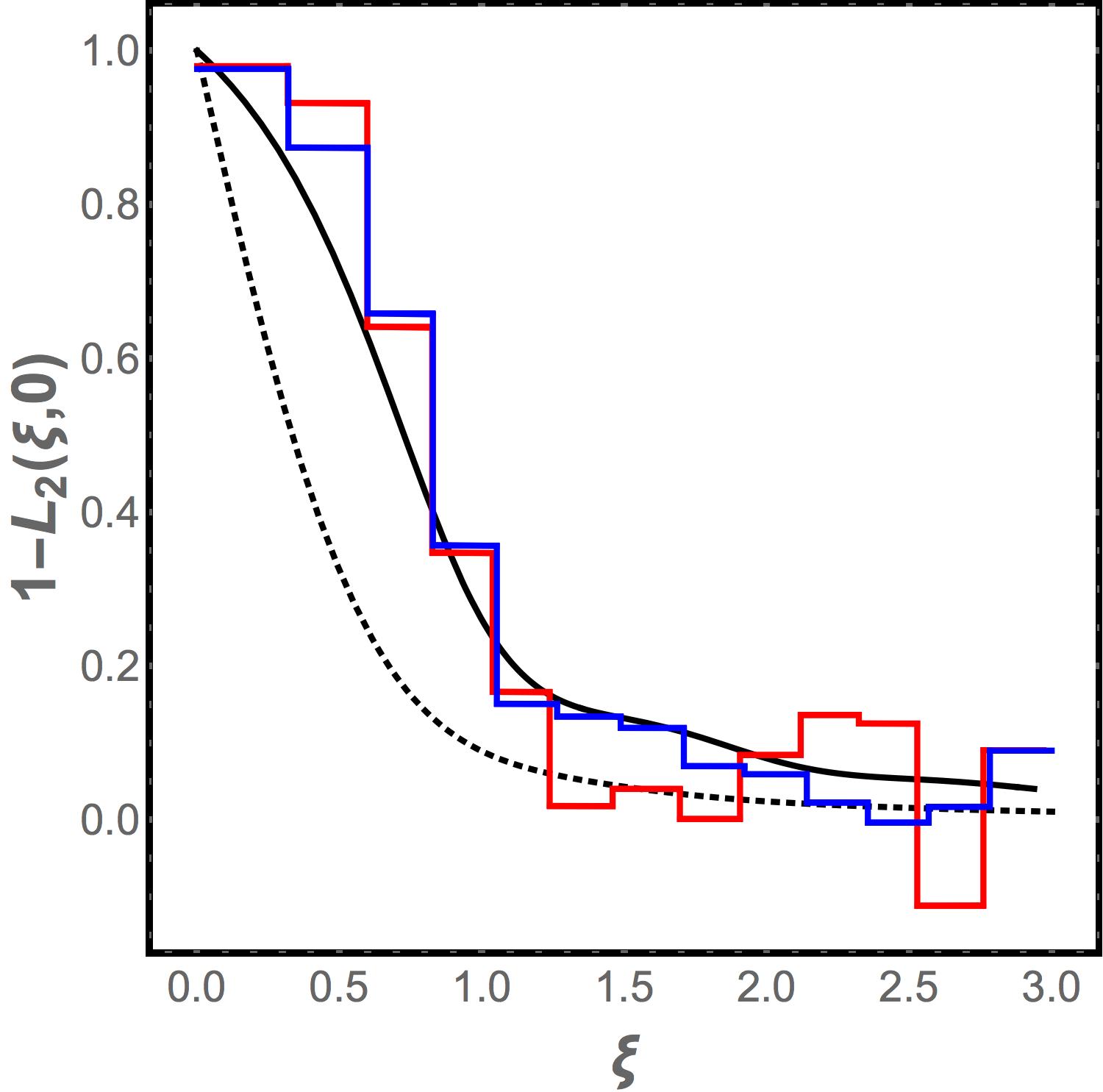
In Figure 2 we plot as a function of for the Laugerre ensemble. The corresponding plot for the Gaussian Orthogonal ensemble is also shown. When is large, the two curves approach each other. Indeed, the analytical expression for for in the Laguerre ensemble can be verified to be
which coincides with the form for the same quantity in the GOE. Intuitively, the reason for this coincidence can be understood in terms of the plasma analogy. If the particles are deep in the interior of the plasma the edge effects produced by the image charges are screened and the Laguerre plasma becomes indistinguishable from the GOE plasma.
Although the two curves coincide in the asymptotic limit , Fig 2 shows that there is a range of values where the predictions of the Laguerre ensemble differ significantly from the GOE. Hence comparison to the correlation function for the numerical data for the jammed granular spectrum provides a stringent test that is able to distinguish between the Laguerre ensemble and the GOE.
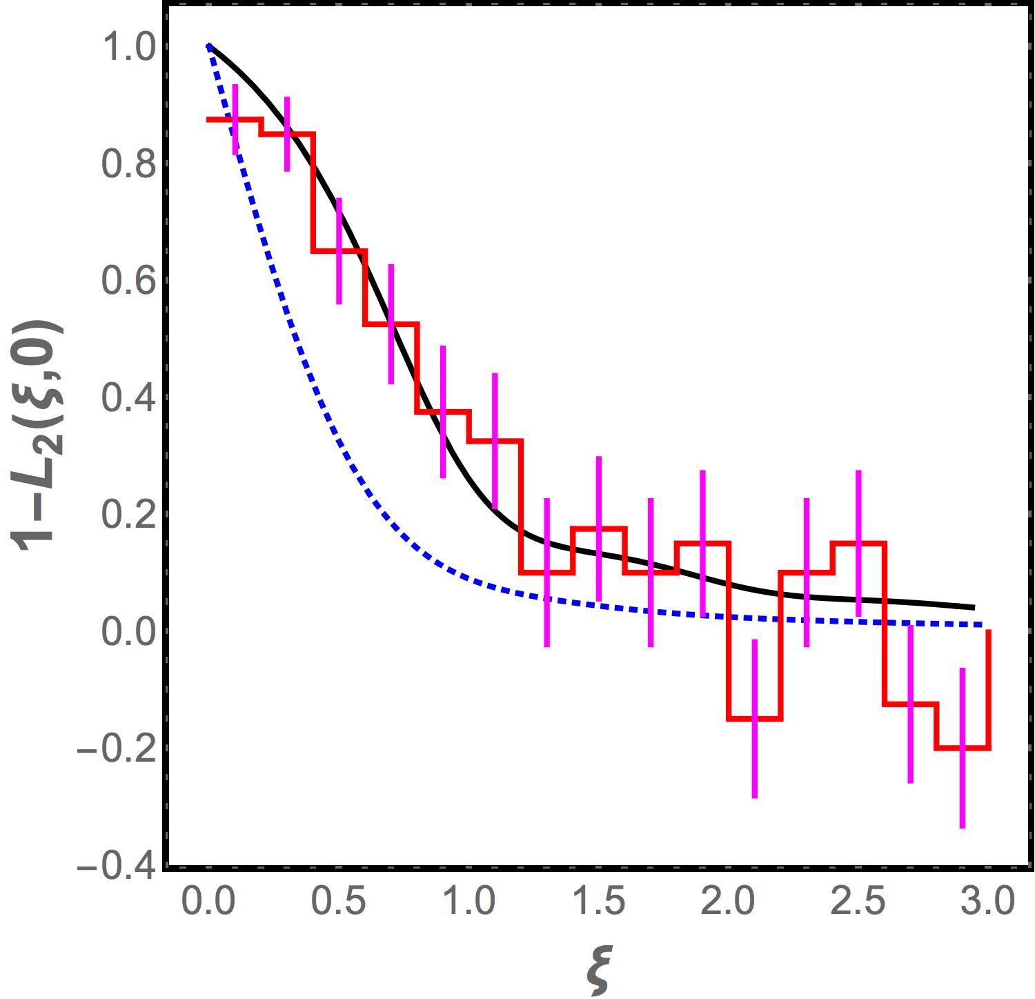
The numerical data are analyzed as follows. The vibrational frequencies obtained in the numerical simulations from all the 1000 realizations of the jammed state are merged together, and bins are constructed with 200 eigenvalues in each, i.e. there is an average of 0.2 eigenvalues per realization of the jammed state in each bin. Next, we calculate
| (19) |
where is the number of vibrational frequencies in the bin in any given realization, and the average is over the realizations of the jammed state. The histogram of the values obtained for this discretized correlation function are compared with the analytical prediction from the Laugerre ensemble and the GOE, and as seen in Fig. 2, the Laguerre ensemble fits the data very well within the error bars (while the GOE does not).
IV Random Lattice Model
As discussed earlier, the extent to which the density of vibrational frequencies for jammed granular materials agrees with the predictions of random matrix theory is not a good test of the applicability of random matrix theory to these materials, because the distribution of eigenvalues is a non-universal prediction of random matrix theory: if the random matrices are not assumed to be Gaussian, the density of eigenvalues changes.
Nevertheless, there are qualitative discrepancies between the numerically measured and the density of eigenvalues obtained from random matrix theory, that are worth trying to address. As seen in Eq.(11), there is a gap in the spectrum of eigenvalues near above the jamming transition, where in Eq.(11). By contrast, in the numerical simulations, is only zero at (except at the jamming transition), and increases linearly for small Second, at the jamming transition, has a cusp-like peak at while random matrix theory predicts a flat near at the transition. Finally, the numerical has a pronounced boson peak at which is not reproduced by random matrix theory.
Various attempts have been made to construct random matrix models that reproduce the properties of granular systems more closely. Ref. Manning studies several different random matrix ensembles and their effect on the structure of eigenmodes with frequencies in the boson peak. Ref. Middleton uses weighted Laplacian dynamical matrices to reproduce an intermediate regime in (between the boson peak and the low frequency behavior) and scaling of the density of states in this regime. Ref. Beltukov1 uses a combination of a random and a regular matrix for the dynamical matrix, to eliminate the gap near Also, Ref. Parisi has studied an abstract model that they argue is in the appropriate universality class.
In Eq.(4), we have assumed that the entries in the matrix are all independent random variables drawn from a Gaussian distribution. In reality, since the matrix is supposed to be a mapping from coordinates to contact forces, and only two particles are associated with a contact, only the entries associated with two particles (with entries per particle for -dimensional particles) should be non-zero in any column of . Thus should be a sparse matrix.
One could choose the two particles associated with each force randomly, but this would result in the system breaking up into separate clusters, not connected to each other, leading to an overabundance of zero modes. Moreover, the concept of adjacency would not be respected: two randomly chosen particles would be likely to be far apart, and should not have been allowed to share a contact.
Instead of choosing the particles associated with a force randomly, we approximate the system as being equivalent to a triangular lattice (with periodic boundary conditions), but with each particle displaced from the position where it would be in a perfect triangular lattice. This randomizes the orientation of the contacts between particles.
To be specific, particles are arranged in successive horizontal layers, with each particle having contacts with the two particles immediately below it: slightly to the left and slightly to the right. Shifting the numbering in each row by half a lattice spacing relative to its predecessor, the particle connects to the particles numbered and with periodic boundary conditions in both directions. (A particle in the bottom layer, connects with and in the topmost layer, where is the number of layers.) In addition, each particle has a probability of connecting to its neighbor on the right in the same row: All contacts are bidirectional, i.e. each particle is connected to two particles in the row above it, two in the row below it, and either zero, one or two adjacent particles in the same row. The spring constant associated with each contact is chosen randomly, and the bond angles are also chosen randomly with the constraint that the bond connecting a particle to its left (right) neighbor in the row below points down and to the left (right), while the bond connecting a particle to its neighbor in the same row on the left (right) is more horizontal than the bond to its neightbor below and to the left (right). This model is similar to the model introduced for free-standing granular piles Narayan , a vector generalization of the scalar-force “q-Model” used to model such systems Coppersmith .
This Random Lattice Model (RLM) with sites was simulated in this manner, and the vibrational frequencies from 100 different realizations of randomness were merged and plotted as a histogram. In two-dimensions, the number of coordinate degrees of freedom is which is comparable to the 800 frequencies that were present in each system in the dynamical simulations Corey . The ratio of the number of contact forces to the number of coordinate degrees of freedom, which corresponds to increases from 1 to 1.5 as the probability of establishing contacts within the same layer increases from 0 to 1.
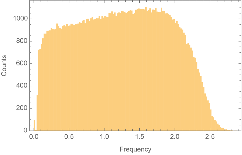
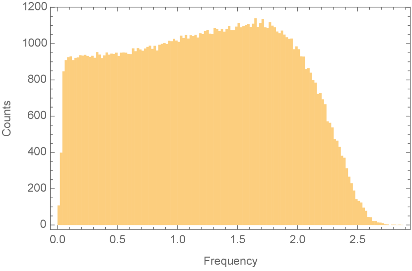
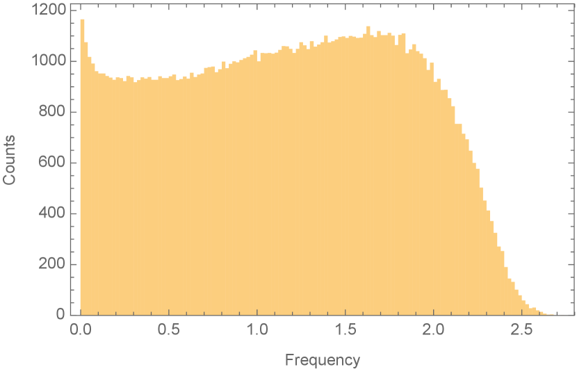
The results are shown in Figure 3. The transition from when to when which is seen in random matrix theory and in the dynamical simulations, is also seen in the RLM density of states. But in addition, there is a cusp in at the transition point, as is seen in the dynamical simulations Corey . The boson peak at seen in the simulations is also reproduced for the lattice model, being most pronounced at the transition point.
Although there is still a gap in the Random Lattice Model frequency spectrum near it is approximately half what one would predict from random matrix theory for the corresponding Moreover, it is clear that it is a finite size effect: the global translational invariance of the random lattice with periodic boundary conditions ensures that there are two zero modes (seen clearly in the first plot in Figure 3), and the locality of the connections that are made ensures that long wavelength oscillations have low frequencies. This is verified by increasing and checking that the gap decreases even though is held constant.
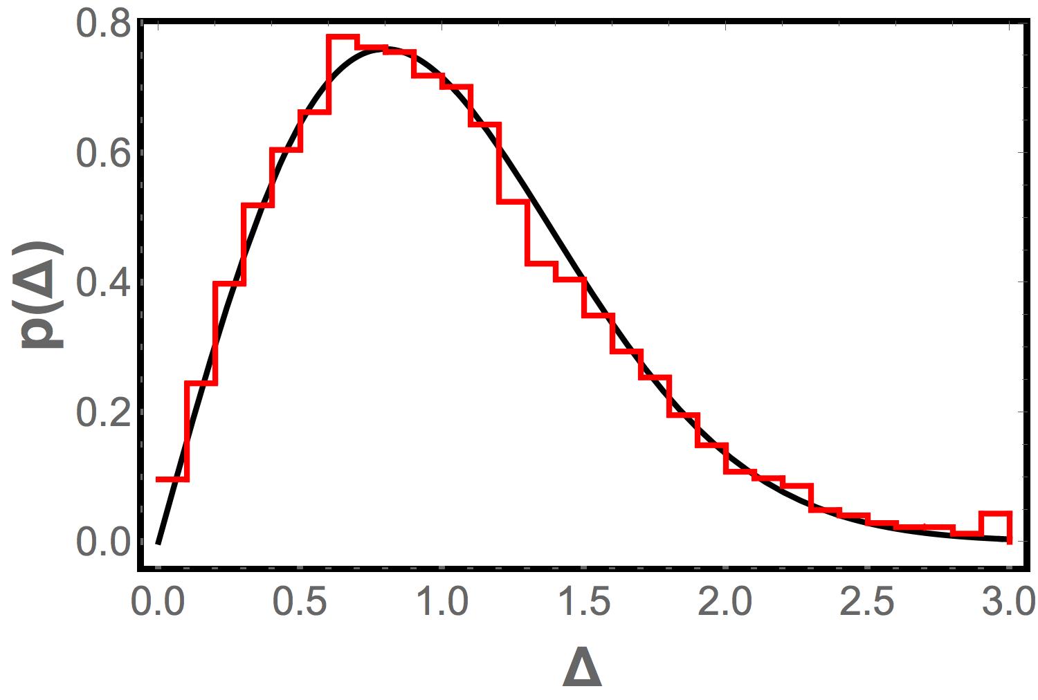
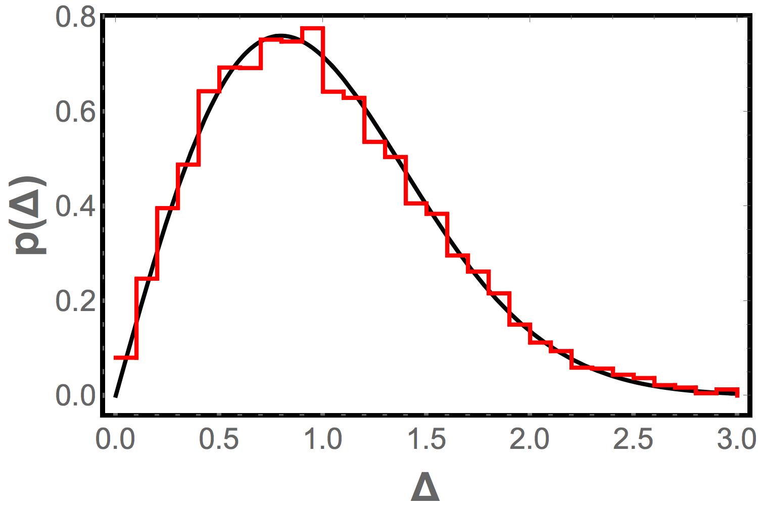
We see that the Random Lattice Model has the same change in at the jamming transition that is seen in the dynamical numerical simulations and in random matrix theory. However, it also reproduces other qualitative features of the numerical that random matrix theory did not. As seen in Figure 4 and in Figure 5, the distribution of spacings between consecutive frequencies is found to be the same as for the random matrix ensemble, consistent with the Wigner surmise, and the correlation function at matches that obtained for the Laguerre ensemble. Thus the random lattice model retains the positive features of random matrix theory, while curing its problems.
V Conclusions
In this paper, we show that a random matrix approach can be used successfully to calculate the correlations between vibrational frequencies in a granular system near the jamming transition, if the matrix ensemble is chosen correctly. By modifying the random matrices according to physical considerations, a Random Lattice Model is constructed, which retains the correlation functions of random matrix theory and also successfully reproduces all the qualitative features in the density of vibrational frequencies. Such random lattice models may be more broadly applicable to granular materials.
Acknowledgements.
The authors gratefully acknowledge data provided by Kyle VanderWerf and Corey O’Hern for numerical simulations on granular systems, to which the models in this paper were compared. Useful conversations with Satya Majumdar are also acknowledged.Appendix A Level spacing distribution
In this Appendix we argue that the distribution of consecutive level spacings for the Laguerre ensemble Eq. (5) is indistinguishable from the GOE. To this end it is useful to recall that for the GOE, Wigner showed that a very good approximation to the level spacing distribution can be obtained by considering a model with just two levels. This formula, known as the Wigner surmise, is indistinguishable from the exact result, except in the tails of the distribution where, in any case, the weight is negligible, making the distinction irrelevant for applications. Intuitively Wigner’s surmise works because at small spacing the distribution is dominated by the interaction between the two consecutive levels; the other levels that are neglected in the analysis only matter at large spacings. In the same spirit we consider the distribution Eq. (5) for the case . We define as the spacing and as the mean energy of the two levels, and we take . For a fixed the level spacing distribution is then given by
| (20) |
for and for . Imposing the condition that the distribution is normalized and rescaling the level spacing so that we obtain the analog of the Wigner surmise for the ensemble in Eq. (5). Because all the integrals can be worked out in closed form, an explicit but extremely lengthy formula can be given for with appropriate normalization and scaling. For the sake of brevity we omit this formula but show in Fig.6 a plot of for fixed . The distribution is essentially indistinguishable from the Wigner surmise for the Gaussian orthogonal ensemble. The deviation over the range of the plot and hence invisible to the eye at the resolution of the figure. is a measure of how close the two consecutive levels are to the edge; to be precise is the ordinal number of the pair whose spacing distribution is being considered; here is the mean density of states corresponding to the distribution in Eq. (5). As one might expect the distribution approaches that for the Gaussian orthogonal ensemble as increases. More surprisingly and perhaps disappointingly we find that for pairs of levels that are quite near to zero frequency also the Gaussian orthogonal ensemble is a good approximation. This means that in testing whether the spectrum of jammed granular matter is described by random matrix theory we cannot use the level spacing to distinguish between our model and the Gaussian orthogonal ensemble.
Since the derivation of the level spacing distribution above is non-rigorous we have tested it by directly simulating our random matrix model. To this end we generated an ensemble of ten thousand random matrices with . The matrix elements are drawn from a Gaussian distribution with zero mean and unit variance. We then evaluated the eigenvalues, of . Fig. 6 shows a histogram of the spacing between the fifth and sixth levels, , in the different realizations. Those spacings have been scaled to have unit mean. As can be seen from the figure the level spacing distribution derived here as well as the distribution for the Gaussian orthogonal ensemble provide an excellent fit to the numerical data. Using the numerical data we were also able to test that the distribution for higher levels is practically indistinguishable, confirming all the features of the analysis above.
It is possible to derive an exact expression for the level spacing distribution using the technology of quaternion determinants developed by Dyson dyson and Mehta mehta and generalized to the Laguerre ensemble by Nagao and Slevin nagao . This analysis would allow a more careful study of the tails of the distribution where it might deviate from the simple approximation derived here. Such an analysis is not needed for the application considered in this paper but is of intrinsic mathematical interest and we will return to it elsewhere.
Appendix B Correlations of the Laguerre Ensemble
Nagao and Slevin nagao have shown that the correlations for the Laguerre ensemble Eq. (13) can be computed by rewriting the distribution as a quaternion determinant and performing the required integrals using a powerful generalization of a theorem by Dyson dyson . Here we summarize their results, taking the opportunity to correct some typos in their paper, and to present the results in a form that does not require the reader to have familiarity with the specialized language of quaternion determinants or Pfaffians.
We start by defining the unfolding function
| (21) |
Note that the order of the Bessel function in the first term of the integrand above is given incorrectly in Ref. nagao .
Next we define
| (22) |
and
| (23) |
In terms of these functions one can write down
| (24) |
where it is understood that is short for and for , the inverse of the function given by Eq. (21). We also write
| (25) |
where denotes the unit step function and
| (26) |
the variable of integration and the arguments of the integrand in Eq. (25) are given incorrectly in Ref.nagao .
With these definitions established we can now write down the principal result of Nagao and Slevin nagao namely
| (27) | |||||
We are interested in . For this special case we obtain the simplifications
| (28) |
Eqs. (27) and (28) are the principal results needed for our test of the random matrix model.
Fig.7 shows a plot of (solid black curve) as well as the corresponding correlation for the GOE (dotted black curve) which is given by the expression in Eq. (LABEL:eq:goetwopoint). We have also computed the correlation function for the ensemble of ten thousand spectra drawn from the Laguerre ensemble as described in in Appendix A. This is shown as the blue histogram. Since these spectra correspond to the very ensemble for which the solid curve represents the exact solution the reason for any departure from the analytic result must be attributed to the finite width of the bins used in analyzing the numerical data and in the finite size of the sample of spectra. This is confirmed by the red histogram which is based on a smaller ensemble of one thousand spectra and shows markedly bigger departures from the analytic result especially for larger . Comparing the red histogram in Fig. 7 to the histogram in Fig. 2 we see that the two agree about equally well with the analytic curve showing that the Laguerre ensemble prediction is indeed in excellent agreement with the numerical data for the vibrational spectrum of jammed granular packs. In more detail the histograms are calculated as follows. We generate an ensemble of random matrices where and is the number of realizations in the ensemble. We then compute the eigenvalues of and denote them where . The range over which the eigenvalues lie is divided into bins and the calculated spectra are binned. Denoting by the number of levels in bin in realization we then compute
| (29) |
is the unfolded width of the bin. The density of states correlator between different bins is then estimated by
| (30) |
then corresponds to over the interval
| (31) |
References
- (1) C.-H. Liu et al, Science 269, 513 (1995); S.N. Coppersmith et al, Phys. Rev. E 53, 4673 (1996).
- (2) M.E. Cates, J.P. Wittmer, J-P. Bouchaud and P. Claudin, Phys. Rev. Lett. 81, 1841 (1998).
- (3) M. van Hecke, J. Phys: Cond. Mat. 22, 033101 (2009).
- (4) D. Bi, J. Zhang, B. Chakraborty and R.P. Behringer, Nature 480, 355 (2011).
- (5) I. Goldhirsch and G. Zanetti, Phys. Rev. Lett. 70, 1619 (1993).
- (6) T.P.C. vanNoije and M.H. Ernst, Granular Matter 1, 57 (1998).
- (7) P.M. Reis, R.A. Ingale and M.D. Shattuck, Phys.Rev. E 75, 051311 (2007).
- (8) F. Rouyer and N. Menon, Phys. Rev. Lett. 85. 3676 (2000).
- (9) M.A. Hopkins and M.Y. Louge, Phys. Fluids A 3, 47 (1991).
- (10) S. McNamara and W.R. Young, Phys. Rev. E 50, R28 (1994).
- (11) E. Brown and H.M. Jaeger, Rep. Prog. Phys. 77, 046602 (2014).
- (12) A.J. Liu and S.R. Nagel eds., Jamming and rheology: constrained dynamics on microscopic and macroscopic scales. (CRC Press, 2001.)
- (13) A.J. Liu and S.R. Nagel, Nature 396, 21 (1998).
- (14) C.S. O’Hern, L.E. Silbert, A.J. Liu and S.R. Nagel, Phys. Rev. E 68, 011306 (2003).
- (15) W.G. Ellenbroek, E. Somfai, M. vanHecke, W.I.M. van Saarloos, Phys. Rev. Lett. 97, 258001 (2006).
- (16) M. Wyart, S.R. Nagel and T.A. Witten, Europhys. Lett. 72, 486 (2005).
- (17) Y.M. Beltukov, JETP Lett. 101, 345 (2015).
- (18) M.L. Mehta, Random Matrices. (Academic Press, San Diego, 1991).
- (19) T. Nagao and K. Slevin, “Laguerre ensembles of random matrices: Nonuniversal correlation functions”, J. Math. Phys. 34, 2317 (1993).
- (20) L.E. Silbert, A.J. Liu and S.R. Nagel, Phys. Rev. E 79, 021308 (2009).
- (21) Z. Zeravcic, W. van Saarloos and D.R. Nelson, Europhys. Lett. 83, 44001 (2008).
- (22) C.L. Kane and T.C. Lubensky, Nat. Phys. 10, 39 (2014).
- (23) C.R. Calladine, Int. J. Solids and Struct. 14, 161 (1978)
- (24) P.J Forrester, Log-Gases and Random Matrices (Princeton University Press, Princeton, 2010).
- (25) K. VanderWerf, A. Boromand, M.D. Shattuck and C.S. O’Hern, Phys. Rev. Lett. 124, 038004 (2020).
- (26) See, e.g., E. Brézin and A. Zee, “Universality of the correlations between eigenvalues of large random matrices”, Nuclear Physics B402, 613-627 (1993)
- (27) F.J. Dyson, Comm. Math. Phys. 19, 245 (1970).
- (28) M.L. Manning and A.J. Liu, Europhys. Lett. 109, 36002 (2015).
- (29) E. Stanifer, P.K. Morse, A.A. Middleton and M.L. Manning, Phys. Rev. E 98, 042908 (2018).
- (30) Y.M. Beltukov, V.I. Kozub and D.A. Parshin, Phys. Rev. B 87, 134203 (2013).
- (31) S. Franz, G. Parisi, P. Urbani and F. Zamponi, Proc. Nat. Acad. Sci. 112, 14539 (2015).
- (32) O. Narayan, Phys. Rev. E 63, 010301 (2000).