Vibrationally-excited Lines of HC3N Associated with the Molecular Disk
around the G 24.78+0.08 A1 Hyper-compact H II Region
Abstract
We have analyzed Atacama Large Millimeter/submillimeter Array Band 6 data of the hyper-compact H II region G 24.78+0.08 A1 (G 24 HC H II) and report the detection of vibrationally-excited lines of HC3N (, ). The spatial distribution and kinematics of a vibrationally-excited line of HC3N (, , ) are found to be similar to the CH3CN vibrationally-excited line (), which indicates that the HC3N emission is tracing the disk around the G 24 HC H II region previously identified by the CH3CN lines. We derive the 13CH3CN/HC13CCN abundance ratios around G 24 and compare them to the CH3CN/HC3N abundance ratios in disks around Herbig Ae and T Tauri stars. The 13CH3CN/HC13CCN ratios around G 24 () are higher than the CH3CN/HC3N ratios in the other disks () by more than one order of magnitude. The higher CH3CN/HC3N ratios around G 24 suggest that the thermal desorption of CH3CN in the hot dense gas and efficient destruction of HC3N in the region irradiated by the strong UV radiation are occurring. Our results indicate that the vibrationally-excited HC3N lines can be used as a disk tracer of massive protostars at the HC H II region stage, and the combination of these nitrile species will provide information of not only chemistry but also physical conditions of the disk structures.
1 Introduction
Massive stars () play essential roles in the evolution and characterization of galaxies, because they produce and disperse large amounts of energy and heavy elements. However, the formation processes of massive stars remain uncertain (see, e.g., Tan et al., 2014, for a review). One formation scenario is the Competitive Accretion model, in which massive stars need to form in clustered environments (Bonnell et al., 2001; Wang et al., 2010). Another is the Turbulent Core Accretion model, a scaled-up version of the formation process of low-mass stars (e.g., McKee & Tan, 2002, 2003), and which can be applied to both clustered and isolated environments. Theoretical models further investigated stellar feedback from forming massive stars (e.g., disk wind, radiation pressure, photoevaporation, and stellar winds) in the Core Accretion model (e.g., Tanaka et al., 2016, 2017). In order to reveal the formation process of massive stars and test the theoretical models, high-angular-resolution and high-sensitivity observations are important (Zhang et al., 2019b, c). In particular, observations of molecular lines are essential, because they provide information about not only gas kinematics but also chemical composition, which is an important tracer of physical conditions and evolutionary stage (e.g., Caselli & Ceccarelli, 2012; Jørgensen et al., 2020; Taniguchi et al., 2019b, 2021b).
Recent high-angular-resolution observations with interferometers such as the Atacama Large Millimeter/submillimeter Array (ALMA) have revealed the presence of disk structures around O-type and B-type massive protostars (Cesaroni et al., 2017; Maud et al., 2018; Zhang et al., 2019a). Tanaka et al. (2020) detected the high-temperature components of disks, which are located at very close distances to massive protostars ( au scale), using several molecular lines such as H2O (), NaCl, SiO, and SiS toward the O-type-binary system IRAS 16547-4247 with ALMA. However, the detailed physical and chemical properties of such disk structures around massive protostars are still unclear. The CH3CN lines are typically used as a disk tracer (Sánchez-Monge et al., 2013; Johnston et al., 2015; Ilee et al., 2016), and sometimes the SiO lines have been used (e.g., Maud et al., 2018; Zhang et al., 2019a).
Nitrile species, CH3CN and HC3N, have been frequently detected in disks around Herbig Ae and T Tauri stars (Bergner et al., 2018; Loomis et al., 2018). The Molecules with ALMA at Planet-forming Scale (MAPS; Öberg et al., 2021) Large Program reveals that these nitrile species trace different layers of these disks; HC3N traces upper and warmer layers compared to CH3CN (Ilee et al., 2021). In disks around Herbig Ae and T Tauri stars, CH3CN is considered to mainly form on dust surfaces followed by the photodesorption or the thermal desorption, while HC3N forms in the gas phase (Loomis et al., 2018; Le Gal et al., 2019). Based on the rotational temperatures of CH3CN, the photodesorption is suggested to be more important than the thermal desorption in these disks (Loomis et al., 2018). Hence, it is useful for investigating physical conditions of disks to observe various nitrile species.
In the case of more massive stars, the CH3CN lines have been frequently used for searching for disks around massive stars (e.g., Johnston et al., 2015; Cesaroni et al., 2017; Sanna et al., 2021), whereas fewer studies about the HC3N lines have been conducted. The vibrationally-excited lines of HC3N have been detected in compact hot cores around massive protostars (e.g., Wyrowski et al., 1999; Taniguchi et al., 2020), but it was still unclear whether these lines trace massive protostellar disks due to the insufficient angular resolutions of those observations. Other higher angular-resolution ALMA data ( au) show that an HC3N vibrationally-excited line (, ; K) traces an accretion disk around the massive protostar in G328.2551-0.5321 (Csengeri et al., 2018). Their result suggests that the vibrationally-excited lines of HC3N could be a tracer of disks around massive young protostars. In order to confirm this hypothesis, it is essential to investigate massive protostars in various evolutionary stages (e.g., hyper-compact H II regions). In addition, the HC3N chemistry in disk structures around massive protostars has not been discussed yet.
In this paper, we present results of two vibrationally-excited HC3N (, , and ) lines detected from the G 24.78+0.08 A1 hyper-compact H II (hereafter G 24 HC H II) region obtained in an ALMA Cycle 6 program. The bolometric luminosity and distance of this source are and kpc, respectively (Moscadelli et al., 2021). We adopt a distance of 6.7 kpc to the G 24 HC H II region (Moscadelli et al., 2021). This source contains a thin shell ionized by an O9.5 star, which was suggested based on studies of the continuum emission and the hydrogen recombination lines (Cesaroni et al., 2019). Moscadelli et al. (2021) found that CH3CN lines are consistent with a Keplerian rotation around a 20 star along the axis PA=133°(disk major axis), while an ionized jet has been identified along the axis at PA=39° at the G 24 HC H II region.
The structure of this paper is as follows. We describe the archival data set and reduction procedure in Section 2. The resultant moment 0 maps of the molecular lines are presented in Section 3.1. The position-velocity (P-V) diagrams are constructed and kinematics of HC3N and CH3CN are investigated in Section 3.2. We describe spectral analyses of the 13CH3CN and HC13CCN lines and derive the CH3CN/HC3N abundance ratios around the G 24 HC H II region in Sections 3.3.1 and 3.3.2, respectively. The CH3CN/HC3N ratios in G 24 are compared to those in disks around Herbig Ae and T Tauri stars in Section 3.3.3. We will discuss the possibility of a binary system in this source in Section 3.4. In Section 4, the main conclusions of this paper are summarized.
2 ALMA Archival Data and Reduction Procedure
We have analyzed the ALMA Band 6 archival data toward the G 24 HC H II region111Project ID; 2018.1.00745.S, PI; Luca Moscadelli. The observations were conducted using the 12-m array on July 29 2019 during Cycle 6. Details of the observations are described in Moscadelli et al. (2021).
We conducted data reduction and imaging using the Common Astronomy Software Application (CASA; McMullin et al., 2007) on the pipeline-calibrated visibilities. We ran the calibration script using CASA version 5.6.1. The data cubes were created by the tclean task in CASA. Briggs weighting with a robust parameter of 0.5 was applied. Pixel size and image size are 0016 and 3500 3500 pixels, respectively. The coordinate of the phase center is (, ) = (18h36m12661, -07°12′1015). The maximum baseline length is 8547.6 m. The field of view (FoV) and maximum recoverable scale (MRS) are approximately 26″and 08, respectively.
Molecular lines and a recombination line presented in this paper are summarized in Table 1. Two vibrationally-excited lines of HC3N (, , and ), which are of our main interest, were observed in the same spectral window. These vibrationally-excited HC3N lines have high upper state energy of – K, which makes them suitable for tracing inner hot gas near the central star, i.e., the disk. In addition to the HC3N lines, we present the data of the CH3CN (, ) line222The detail studies of this line are summarized in Moscadelli et al. (2021). that has a similar upper state energy to the HC3N (, ) lines. We will compare their spatial distributions and P-V diagrams in order to confirm that the HC3N lines trace the disk structure around the G 24 HC H II region. We also made data cubes of vibrationally ground-state lines of 13CH3CN (, ) and HC13CCN (, ), which are expected to be optically thin, in order to derive their column densities (Section 3.3.1). The data cube of the H30 line is presented in Section 3.4 to discuss a possibility of the binary system. The velocity resolution of these data is 0.63 km s-1.
Continuum image ( mm) was created from the broadest spectral window (1.9 GHz bandwidth, center frequency of 217.8 GHz) using the imcontsub task in CASA. Since some lines have been detected at the HC H II region position in this spectral window, we determined line-free channels in the tclean image for the imcontsub task. The polynomial order of 0 was adopted for the continuum estimation. The rms noise level of the continuum image is 0.1 mJy beam-1.
| Species | Transition | Frequency | |
|---|---|---|---|
| (GHz) | (K) | ||
| HC3N ()aaRest frequencies were taken from the Cologne Database for Molecular Spectroscopy (CDMS; Müller et al., 2005). | , | 219.6751141 | 773.5 |
| , | 219.7073487 | 776.8 | |
| HC13CCN ()aaRest frequencies were taken from the Cologne Database for Molecular Spectroscopy (CDMS; Müller et al., 2005). | 235.5094856 | 152.6 | |
| CH3CN ()bbRest frequency was taken from the JPL database (Pickett et al., 1998). | 221.3118349 | 771.1 | |
| 13CH3CN ()aaRest frequencies were taken from the Cologne Database for Molecular Spectroscopy (CDMS; Müller et al., 2005). | 232.0772032 | 335.5 | |
| 232.1251297 | 256.9 | ||
| 232.1643692 | 192.5 | ||
| 232.1949056 | 142.4 | ||
| 232.2167263 | 106.7 | ||
| 232.2298223 | 85.2 | ||
| 232.2341883 | 78.0 | ||
| CH3CN ()bbRest frequency was taken from the JPL database (Pickett et al., 1998). | 220.6792869 | 183.1 | |
| H30 | … | 231.900928 | … |
3 Results and Discussion
3.1 Spatial distributions of molecular lines
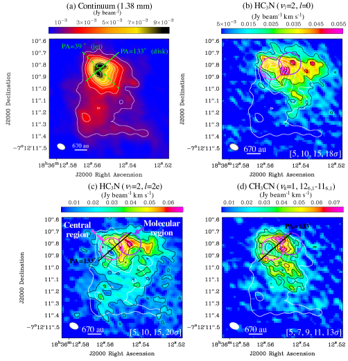
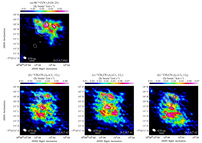
We show the continuum image ( mm) toward the G 24 HC H II region in panel (a) of Figure 1, which was first reported by Moscadelli et al. (2021). The angular resolution is 0071 0048, corresponding to 476 au 322 au at the source distance of 6.7 kpc. The beam position angle (PA) is 63.9°. Two peaks are located at the center, and the spatial distribution of the continuum emission is slightly elongated along the north-east to south-west direction (PA = 39°). We will discuss a possible reason for the two peaks in the continuum emission in Section 3.4. Another continuum core is located 04 (2680 au) south of the strongest continuum core. This position is consistent with A1M (a molecular emission peak position) named by Moscadelli et al. (2018), and they found that column densities of several complex organic molecules (COMs) are abundant here.
Panels (b)–(d) of Figure 1 show the moment 0 maps of three vibrationally-excited molecular lines; (b) HC3N (, , ), (c) HC3N (, , ), and (d) CH3CN (, ); toward the G 24 HC H II region. We select two areas for our analysis, namely “Central region” and “Molecular region” (panel (c) of Figure 1). The central position of the Central region corresponds to the middle of the two continuum peaks, and that of the Molecular region is at the peak position of the HC3N (, , ) line, respectively. Their coordinates are (, ) = (18h36m12556, 07°12′1085), and (18h36m12546, 07°12′1080), respectively. The other molecular lines also have peaks within the Molecular region. We selected the two regions to investigate the potential chemical variation induced by different UV fluxes, which is expected to be higher in the Central region. The Central region is the same position that Moscadelli et al. (2021) analyzed. Following their work, we adopt the radii of 01 for the two regions, which allows us to check the consistency between their and our analyses (see Section 3.3.1).
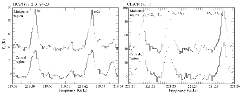
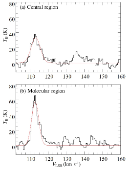
Figure 2 shows the spectra of the HC3N and CH3CN lines at the Central and Molecular regions. Other two CH3CN lines (, and ) are also detected near the CH3CN (, ) line. We checked molecular lines in the Splatalogue database333https://splatalogue.online//advanced1.php, and found that no other lines are likely to contaminate the spectra. In addition, the two vibrationally-excited lines of HC3N show similar intensities and spatial distributions as expected. We thus concluded that line contamination does not occur.
In the moment 0 maps (panels (b) – (d) of Figure 1), we can recognize the overall similarities in the spatial distributions of the HC3N and CH3CN emissions. Their emission regions have similar extents of , because they have almost the same upper state energies of K (Table 1; see also Figure 6 of Moscadelli et al., 2021). Also, all three emissions are dimmer in the Central region, probably due to photodissociation by intense UV flux (see also Section 3.3.2). These similarities suggest that the vibrationally-excited HC3N and CH3CN lines trace the same hot, dense region surrounding the central ionized region, i.e., the molecular disk reported by Moscadelli et al. (2021). We note, despite these similarities, the HC3N and CH3CN lines also show a difference in their emission morphology. The CH3CN emission surrounds the Central region, while the two HC3N lines are mainly located in the northwest. We can explain this spatial difference if the UV flux from the Central region is stronger toward the south direction, because HC3N would be more efficiently photodissociated than CH3CN (Section 3.3.2). Unresolved asymmetric innermost structures, e.g., clumpy density structure and a presence of a binary system (Section 3.4), could be at the origin of such an anisotropic UV radiation field.
3.2 Kinematics of HC3N and CH3CN
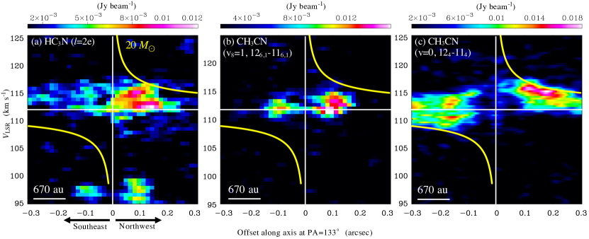
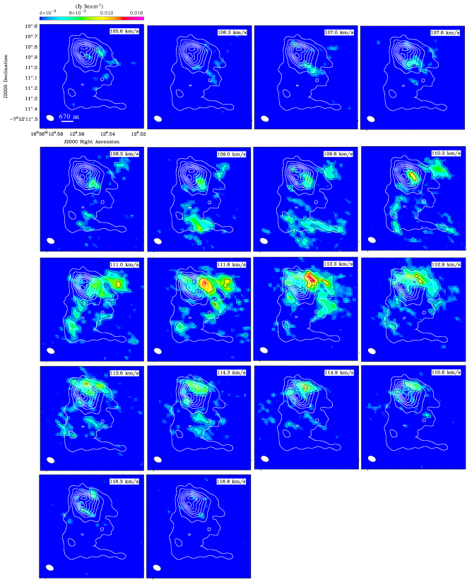
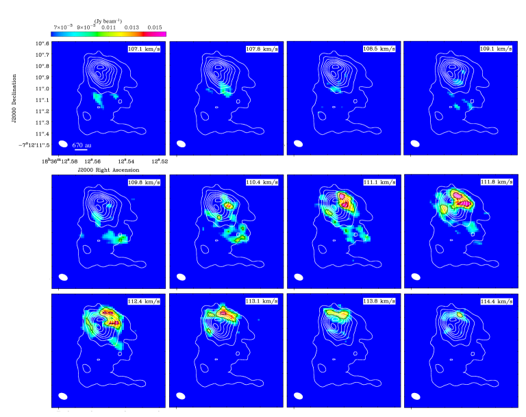
Having confirmed the similarity of the spatial distributions, we next investigate the kinematical similarity of the vibrationally-excited HC3N and CH3CN lines. Moscadelli et al. (2021) reported the Keplerian disk of G 24 using the P-V diagrams of the CH3CN lines, including its vibrationally-excited line and 13C isotopologue line. In order to confirm that the vibrationally-excited HC3N line also traces the same molecular disk, we constructed P-V diagrams of HC3N (, , ) and CH3CN (, ) along the disk major axis of PA=133°(shown in Figure 1). We used “impv” task in CASA, and averaged the emission over three pixels across the positional cut. The center position (offset = 0″) is set at the coordinate of the Central region. Panels (a) and (b) of Figure 3 show the P-V diagrams of the vibrationally-excited HC3N and CH3CN lines, respectively. Their channel maps in Figures 11 and 12 in Appendix B. For comparison, we also provide the P-V diagram of the vibrational ground-state line of CH3CN (), which clearly shows the Keplerian feature with but becomes dimmer in the innermost region (panel (c) of Figure 3).
In the P-V diagrams, we could confirm that the HC3N emission has kinematic similarities with the vibrationally-excited and ground-state CH3CN lines, but the resemblance is stronger to the vibrationally-excited line of CH3CN. The brightest features appear in the northwest and redshifted side, and the dimmest features are in the northwest and blueshifted side in all three panels of Figure 3. On the brightest side, the HC3N emission covers the innermost region of like the vibrationally-excited CH3CN line, which has almost the same upper-state energy (panels (a) and (b)). Moreover, on the same side, the HC3N emission shows the consistent profile as the Keplerian rotation seen in the ground-state CH3CN emission (panels (a) and (c)). Hence, we conclude the vibrationally-excited HC3N line associated with the same Keplerian disk reported by Moscadelli et al. (2021). Although the HC3N emission shows some resemblance to that of CH3CN in the P-V diagrams (Figure 3), the degree of this resemblance is still debatable. Future higher-angular resolution observations including other transitions are necessary for further discussions.
The other similarity is that these HC3N and CH3CN lines show emission features on the southwest and redshifted side of the P-V diagrams (see also Figure 4 of Moscadelli et al., 2021). The distribution of the HC3N emission lines is intermediate between those of the vibrationally-excited and ground-state CH3CN lines. This again supports that the HC3N line traces the same gas as CH3CN. We note that such a kinematical feature cannot be reproduced by a pure Keplerian disk (Sakai et al., 2014; Zhang et al., 2019a). Contamination from an infalling, rotating envelope is able to create this feature, even though we used the lines with the high upper-state energies, which can be excited only in hot dense gas (cf., K and the critical density of for the HC3N line; Wyrowski et al., 1999). One difference between the HC3N and ground-state CH3CN lines appears on the southeast and blueshifted sides in their P-V diagrams (panels (a) and (c)). The HC3N emission is darker on the southwest side, making it difficult to trace that side of the Keplerian feature (see also Figure 1). An anisotropic UV radiation field could create this HC3N depletion, which we also mentioned in Section 3.1. This would imply that fast chemical processes change the chemical composition of the molecular disk with a shorter timescale than the rotational timescale for the disk (e.g., Cleeves et al., 2017).
3.3 The abundances of HC3N and CH3CN
As mentioned in Section 1, HC3N and CH3CN trace different layers of disks around Herbig Ae and T Tauri stars (Ilee et al., 2021), suggesting that these species trace different physical conditions in disk structures. In order to investigate the physical and chemical conditions of the molecular disk around the G 24 HC H II region, we will evaluate the CH3CN/HC3N abundance ratios.
3.3.1 Spectral line analyses of 13CH3CN and HC13CCN
| Central region | Molecular region | ||||
|---|---|---|---|---|---|
| Line | (K) | (km s-1) | (K) | (km s-1) | |
| 13CH3CN () | |||||
| HC13CCN () | |||||
Note. — Errors indicate the standard deviation.
We derive column densities of HC13CCN and 13CH3CN using their vibrational ground-state lines. Figure 10 in Appendix A shows the moment 0 maps of the vibrational ground-state lines of their 13C isotopologues. These lines are usually optically thin, and we can derive their column densities more accurately than the case with the main species.
We obtained the spectra of 13CH3CN and HC13CCN at the Central and Molecular regions over the 01 radius. As described in Section 3.1, the Central region is the same region where Moscadelli et al. (2021) analyzed. The derived column densities and rotational temperatures in this section are the beam-averaged values, as Moscadelli et al. (2021) derived.
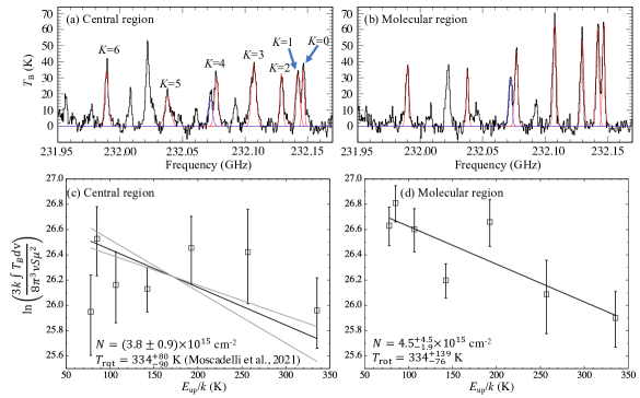
Panels (a) and (b) of Figure 4 show the spectra of 13CH3CN () at the Central and Molecular regions, respectively. We fitted the spectra with a Gaussian profile, and summarized the obtained parameters in Table 2. We analyzed the 13CH3CN spectra with the rotational diagram method using the following formula (Goldsmith & Langer, 1999);
| (1) |
where is the Boltzmann constant, is the line strength, is the permanent electric dipole moment, is the column density, is the rotational temperature, is the upper-state energy, and is the partition function. The permanent electric dipole moment of 13CH3CN is 3.92197 Debye (Gadhi et al., 1995).
Panels (c) and (d) of Figure 4 show results of the rotational diagram analysis at the Central and Molecular regions, respectively. At the Central region, we could not obtain the rotational temperature by the fitting, partly because some lines do not show a Gaussian profile, and then we applied an rotational temperature of K derived by Moscadelli et al. (2021). Their results are applicable, since Moscadelli et al. (2021) analyzed the 13CH3CN spectra at the HC H II region within a 01 radius, which is the same region as we have analyzed. The column density of 13CH3CN at the HC H II region is derived to be () cm-2. This column density is consistent with the previous result within the uncertainties ( cm-2; Moscadelli et al., 2021). The rotational temperature and column density at the Molecular region are derived to be K and cm-2, respectively, by the rotational diagram fitting for our data.
The derived rotational temperatures at the two positions are much higher than the sublimation temperature of CH3CN ( K444We took the sublimation temperature from a hot-core model by Taniguchi et al. (2019a).), which is different from results in the disks around the Herbig Ae and T Tauri stars (Bergner et al., 2018; Loomis et al., 2018; Ilee et al., 2021). Such high rotational temperatures of 13CH3CN indicate that CH3CN, including its isotopologues, thermally desorbs from dust grains rather than photodesorption by the UV radiation around the G 24 HC H II region.
| Central region | Molecular region | |||||
|---|---|---|---|---|---|---|
| (K)aaExcitation temperatures () are taken from the results of 13CH3CN. | (cm-2) | (K)aaExcitation temperatures () are taken from the results of 13CH3CN. | (cm-2) | |||
| 334 | () | 0.107 | 334 | () | 0.195 | |
| 244 | () | 0.151 | 258 | () | 0.262 | |
| 414 | () | 0.086 | 473 | () | 0.133 | |
Note. — Errors indicate the standard deviation.
Figure 5 shows spectra of the HC13CCN () line at the Central and Molecular regions, obtained by the same method as that for 13CH3CN. We fitted the spectra with a Gaussian profile, and the fitting results are shown as red curves in Figure 5. Table 2 summarizes the line parameters obtained by the fitting. The values of this line are km s-1 and km s-1 at the Central and Molecular regions, respectively.
Since we have only one rotational transition line of HC13CCN, we need a reasonable assumption of its excitation temperature to derive its column density. If the emission region of 13CH3CN coincides with that of HC13CCN and the LTE condition is achieved, we can use the excitation temperature of 13CH3CN as the reference value. Therefore, we compare their line widths of 13CH3CN and HC13CCN to examine their spatial coincidence.
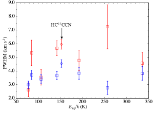
Figure 6 shows relationships between the line width (FWHM) and the upper state energy of the 13CH3CN and HC13CCN lines. We derive the line width (FWHM) using
| (2) |
where and are the observed line widths and the instrumental velocity width (0.63 km s-1), respectively. There are no clear dependencies of the line width on the upper state energy. The value of the line of 13CH3CN and its error toward the Central region are slightly larger than those of the other lines, which may be due to the contamination of another line (panel (a) of Figure 4). The line widths at the Central region are generally larger than those at the Molecular region, and the line widths of the HC13CCN line are comparable to those of 13CH3CN. Thus, we hereafter assume the excitation temperature of HC13CCN is the same as the 13CH3CN’s rotational temperature.
We derived the column densities of HC13CCN at the two positions assuming the LTE condition (Goldsmith & Langer, 1999). We used the following formulae;
| (3) |
where
| (4) |
and
| (5) |
In Equation (3), denotes the optical depth, and the peak intensities summarized in Table 2. and are the excitation temperature and the cosmic microwave background temperature (2.73 K). We calculated three cases of excitation temperatures (, (error)) for each position. () in Equation (4) is the effective temperature equivalent to that in the Rayleigh-Jeans law. In Equation (3.3.1), N is the column density, is the line width, () is the partition function at , is the permanent electric dipole moment, and is the energy of the lower rotational energy level. The electric dipole moment of HC13CCN is 3.732 Debye (CDMS database; Müller et al., 2005).
Table 3 summarizes the derived column densities of HC13CCN and the peak optical depth () at each position. We confirmed that the HC13CCN line is optically thin. The derived column densities at the Molecular region are slightly higher than those at the Central region, as in the case of 13CH3CN (see Figure 4).
3.3.2 The CH3CN/HC3N abundance ratios in G 24
The (13CH3CN)/(HC13CCN) ratios are derived to be and at the Central and Molecular regions, respectively, using the results in Section 3.3.1. If there are no effects of the 13C isotopic fractionation in each molecule (e.g., Taniguchi et al., 2016, 2017) and the selective photodissociation of 13CH3CN and HC13CCN, the (13CH3CN)/(HC13CCN) ratio reflects the CH3CN/HC3N abundance ratio. In the case of G 24 with the strong UV radiation field, it is likely that the effect of the 13C isotopic fractionation of HC3N is negligible (Taniguchi et al., 2019a, 2021a).
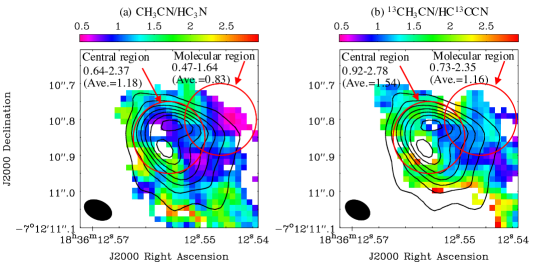
In order to confirm the CH3CN/HC3N abundance ratios around G 24, we investigated the CH3CN/HC3N ratios using the moment 0 maps of their vibrationally-excited lines. These lines have similar upper state energies ( K, Table 1). In addition, the estimated gas density traced by the CH3CN () lines is around cm-3 (Moscadelli et al., 2021), and the critical density of the HC3N () lines is cm-3 (Wyrowski et al., 1999). Hence, these vibrationally-excited lines of CH3CN and HC3N likely trace similar regions around G 24, and their excitation conditions are expected to be equivalent. If these lines are optically thin, this integrated-intensity ratio would be comparable to their abundance ratio. Panel (a) of Figure 7 shows the map of the ratio between the CH3CN moment 0 map (panel (d) of Figure 1) and that of HC3N (panel (c) of Figure 1) toward G 24. We included only pixels with above detection of both species. We also show the same map but between the 13CH3CN () and HC13CCN () lines (panels (c) and (a) of Figure 10, respectively), in order to cross check the results. We used the 13CH3CN () line, because it has the closest upper-state energy to the HC13CCN () line (see Table 1).
The CH3CN/HC3N ratios including their 13C isotopologues cannot be derived near the continuum peak due to the below detection of HC3N, which could indicate the efficient HC3N destruction at the Central region. In panel (a), the CH3CN/HC3N ratio shows lower values in the Molecular region (, the average value is 0.83) compared to those in the Central region (, the average value is 1.18). This marginal difference in the CH3CN/HC3N ratio between the two regions suggests that the UV photodissociation and/or reactions with ions increase the CH3CN/HC3N abundance ratio in the region irradiated by the strong UV radiation. This can be caused by the following two reasons;
-
1.
HC3N could be more efficiently destroyed at the Central region, because the UV photodissociation rate of HC3N is higher than that of CH3CN by a factor of (Table 2 in Le Gal et al., 2019).
-
2.
HC3N is destroyed by reactions with ions (H+, H, HCO+), which should be abundant in ionized regions (Taniguchi et al., 2019a).
The 13CH3CN/HC13CCN ratios are derived to be (the average value is 1.54) and (the average value is 1.16) at the Central and Molecular regions, respectively (panel (b) of Figure 7). The 13CH3CN/HC13CCN ratio at the Molecular region is lower than that at the Central region, as seen in panel (a), and this tendency is also consistent with the (13CH3CN)/(HC13CCN) ratios.
We adopt the (13CH3CN)/(HC13CCN) column density ratio as representative values in G 24 in the following section, because the CH3CN/HC3N ratio based on the moment 0 maps may be affected by the effect of the optically thickness.
3.3.3 Comparisons of the CH3CN/HC3N abundance ratios among the high- and lower-mass protostellar disks
We compare the CH3CN/HC3N abundance ratios in the disk structure of G 24 to those in disks around lower-mass stars, i.e., Herbig Ae stars and T Tauri stars, and investigate chemical properties of the molecular disk around G 24.
In disks around lower-mass stars, a main formation mechanism of CH3CN is considered to be dust-surface reactions (Bergner et al., 2018; Loomis et al., 2018); (1) the successive hydrogenation reaction of C2N and (2) a radical-radical reaction between CH3 and CN. Gas-phase routes have been also investigated (Bergner et al., 2018; Loomis et al., 2018):
| (6) |
followed by
| (7) |
However, Loomis et al. (2018) concluded that the dust-surface routes are more efficient than the gas-phase ones. The CH3CN formed on dust surfaces sublimates into the gas phase by thermal desorption or photo-evaporation. As the excitation temperatures of CH3CN are lower than its sublimation temperature in disks around lower-mass stars, the primary path would be photo-evaporation in such disks.
On the other hand, for HC3N, only gas-phase formation routes are known, including the ion-molecule reactions and the neutral-neutral reactions (Loomis et al., 2018; Le Gal et al., 2019). For example, the following reactions are considered to contribute to the HC3N formation:
| (8) |
or
| (9) |
The HC3NH+ ion is formed by various ion-molecule reactions (e.g., C2H+HCN, C3H+N (); Taniguchi et al., 2016, 2017).
Both CH3CN and HC3N are destroyed by the UV photodissociation:
| (10) |
and
| (11) |
respectively. HC3N is also destroyed by ions, such as H+, H, HCO+, in higher regimes ( mag; Le Gal et al., 2019). The reaction with C+ could destroy CH3CN (Loomis et al., 2018), but its contribution is not dominant in the chemical network simulation conducted by Le Gal et al. (2019).
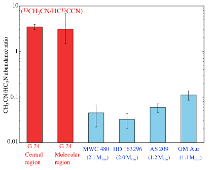
Figure 8 shows comparisons of the CH3CN/HC3N abundance ratio among protostellar disks with different stellar masses. The abundance ratios in Herbig Ae and T Tauri stars are taken from Ilee et al. (2021). MWC 480 and HD 163296 are Herbig Ae stars, and AS 209 and GM Aur are T Tauri stars, respectively. The derived (13CH3CN)/(HC13CCN) ratios around G 24 () are higher than the CH3CN/HC3N abundance ratios in the other disks () by more than one order of magnitude. As discussed in Section 3.3.2, there are differences in the CH3CN/HC3N ratio around the G 24 HC H II region by a factor of a few among different methods, but the CH3CN/HC3N ratios around G 24 are clearly higher than those in the disks around the lower-mass stars.
One possible explanation for the high CH3CN/HC3N abundance ratio around G 24 is that the thermal sublimation mechanism enhances the gas-phase CH3CN abundance around the massive star, while the photo-evaporation is important for sublimation of CH3CN in the other disks. In addition, HC3N could be more efficiently destroyed around the massive star, because of the higher UV photodissociation rate of HC3N than that of CH3CN, as we have already discussed in Section 3.3.2. HC3N is also destroyed by reactions with ions (H+, H, HCO+), which should be abundant in ionized regions.
We also compare the CH3CN/HC3N ratios around G 24 to that of the Orion Hot Core (i.e., envelope scale; Crockett et al., 2014). The Orion Hot Core is associated with Source I, and its mass was estimated to be around 15 (Bally et al., 2020). In addition, the disk structure has been detected around this source (Wright et al., 2020). Thus, it seems to be a good source to compare the chemical composition to G 24. The CH3CN and HC3N abundances with respect to H2 at the Orion Hot Core were derived to be and , respectively ((H2)= cm-2; Crockett et al., 2014). Hence, the CH3CN/HC3N abundance ratio is calculated at 3.7. This value is comparable to the CH3CN/HC3N ratios around G 24 (). The similar CH3CN/HC3N ratios between the Central and Molecular regions in G 24, and between G 24 and the Orion Hot Core imply the following two possibilities:
-
1.
The disk chemistry may be inherited from the envelope.
-
2.
The chemical processes at the envelope scale may be similar to those at the disk scale due to the powerful central source.
Here, we demonstrate the possibility of the different nitrile chemistry between massive stars and lower-mass stars, i.e., Herbig Ae and T Tauri stars. However, we have data of both CH3CN and HC3N toward only one massive star. In order to confirm the nitrile chemistry in disk structures around massive stars, we need to increase source samples. Future observations covering several lines, which enable us to derive accurate column densities and excitation temperatures of CH3CN and HC3N, are necessary to understand the disk chemistry around massive stars. These observations will help us to reveal the massive star formation processes.
3.4 The possibility of a binary system
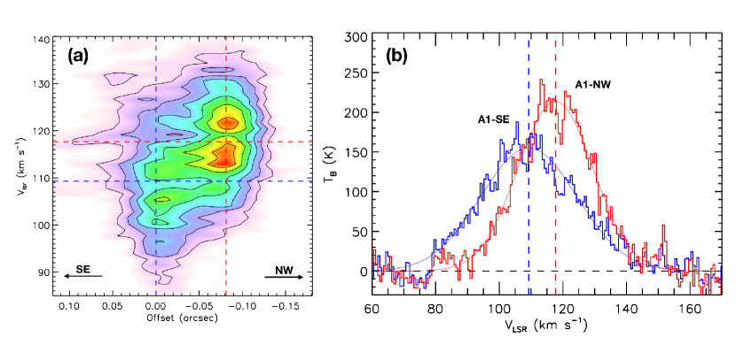
As shown in panel (a) of Figure 1, the two peaks with the separation of are detected in the 1.38 mm continuum emission. Panel (a) of Figure 9 shows the P-V diagram of the H30 emission along a direction connecting the two continuum peaks (). It clearly shows that the H30 emission associated with the southeast peak is blueshifted by from the northwest peak.
Moscadelli et al. (2021) interpreted this velocity gradient as the ionized disk rotation around a massive protostar. Assuming an edge-on orientation, they derived the dynamical mass of , which should be the minimum mass considering the possible inclination. Consistent with this dynamical mass evaluation, Cesaroni et al. (2019) suggested an O9.5 star based on the derived Lyman continuum rate of . We also constructed the spectral energy distribution (SED) toward this source to retrieve the stellar mass and other physical properties, using infrared data from Spitzer, WISE, and Herschel (Table 4 in Appendix C) and fitting the SED with the Zhang & Tan (2018) model (see Appendix C for the details). The best models of the SED fitting suggested the stellar masses of – with the bolometric luminosities of a few times (see Figure 13 and Table 5 in Appendix C), which is also consistent with the dynamical mass estimation with the Keplerian disk by Moscadelli et al. (2021). The agreement of the independent analyses supports the presence of a star with the ionized-gas disk in the center of the G 24 HC H II region.
However, this ionized disk scenario does not explain the presence of the two continuum peaks well. An alternative interpretation would be that the kinematic structure of H30 consists of two ionized disks associated with two massive young stars orbiting around each other, i.e., a binary system. In fact, instead of one single velocity gradient across , the P-V diagram appears to be more consistent with two separate components with the velocity offset (i.e., the orbital motion), each of which has its own velocity gradient (i.e., the rotation of each disk). It is worth briefly discussing the possibility of the binary system in G 24, considering its asymmetric structures and the high binary rate of massive stars.
We can derive the total mass of the binary system assuming that the protostars locate at the continuum peaks and their velocity offset is due to the orbital motion. The peak separation is or , which is a project separation. We estimate their velocity offset as from the H30 spectra at the peak locations (panel (b) of Figure 9). Considering a circular Kepler orbit, we derive the total dynamical mass as , where is the gravitational constant. This formula is different from that in the disk scenario by a factor of 8, i.e., (where is the stellar mass at the disk center; see Sec. 4.1 of Moscadelli et al., 2021), because represents the separation of the two sources while it is the diameter of the ionized disk in the disk scenario. Since free-free and H30 emissions trace the surrounding ionized gas rather than the protostar itself, the actual positions of the protostars might be slightly off the continuum emission peaks. Considering such uncertainty of (or ) and the fitting error of , we estimate that the mass range of – is consistent with the binary scenario. We note that the circular orbit perpendicular to the plane of sky are assumed here, and thus we consider those as the minimum masses.
The total values of the Lyman continuum rate and the infrared luminosity can also provide constraints on the stellar masses of the binary. Moscadelli et al. (2018) and Cesaroni et al. (2019) estimated a total Lyman continuum rate of – by fitting the radio to millimeter SED. Since the two peaks have similar brightness in continuum and H30 total emissions, the two massive stars in the binary should have similar masses, and therefore similar Lyman continuum rate of . Such a Lyman continuum rate corresponds to a zero-age main sequence (ZAMS) mass of , making a total mass of for the binary, which is close to the minimum dynamical mass estimated above. If the binary stars have not reached the ZAMS phase, their masses can be higher because their Lyman continuum rate would be lower than those in the ZAMS phase at the same masses (e.g., Tanaka et al., 2016). As discussed in Appendix C, we conducted the infrared SED fitting. The mass estimation from this fitting is not applicable for the binary system because it assumed a single-star system. However, the obtained total bolometric luminosity of a few is reasonable even for the multiple-source system (Table 5). Considering the protostellar evolution, the luminosity of a massive protostar with – would be as bright as (e.g., Zhang & Tan, 2018), which is again consistent with the estimation of the dynamical mass.
The systemic velocity of G 24 measured from the outer molecular emissions is 112 km s-1. If we assume that the line-of-sight velocity of the mass center of the binary is , the mass ratio between the primary and secondary would be about 2:1 from the central velocity of each continuum peak. Considering the dynamical mass of , we evaluate for A1-SE and for A1-NW. However, such analysis is susceptible to the determination of the line center velocities of H30, which have FWHMs of km s-1, as well as the binary system velocity. Therefore, it is still difficult to accurately determine the masses of the individual stars via dynamics.
We note that the binary scenario does not necessarily contradict the other features of G 24. In the case of the binary star scenario, the rotating structure traced by CH3CN and HC3N is a circumbinary disk surrounding the two massive stars. The P-V diagrams of the molecular lines are roughly consistent with the Keplerian rotation with , but the disk is assumed to be perpendicular to the sky in these diagrams (Figure 3; Figure 4 of Moscadelli et al., 2021). Hence, the value of is the minimum enclosed mass, and the total dynamical mass of from the H30 emission is acceptable. The presence of a single jet perpendicular to the molecular disk reported by Moscadelli et al. (2018, 2021) does not exclude the binary scenario. For example, in the forming massive binary system IRAS 16547–4247, one of the binary stars launches a single jet nearly perpendicular to the circumbinary disk, while the other star shows no jet feature, despite both protostars show almost the same levels of continuum and line emissions (Tanaka et al., 2020). If this is also happening in G 24, one star may be supplied with more material from the circumstellar disk. Such an asymmetric infalling structure at could cause the asymmetric UV field suggested in the larger scale.
Similar to the binary scenario for G 24, Zhang et al. (2019b) reported a forming massive binary IRAS 07299–1651 with each member traced by hydrogen recombination lines showing velocity offset caused by orbital motion. In IRAS 07299-1651, the line emissions from the two stars are well separated that allows analyzing the circumstellar disk rotation of the primary star. However, in G 24, the H30 emissions from the continuum peaks have already spread out and merged together, making it difficult to analyze the detailed kinematic structures of the ionized gas, i.e., the circumstellar disks and their circumbinary disk. We speculate that G 24 is more massive than IRAS 07299-1651, and thus the ionized gas is more extended. Therefore, although we suggest the possibility of the binary system in G 24, we cannot confirm such a scenario with the current data set. Future higher-angular-resolution observations may help to confirm this point.
4 Conclusions
We have analyzed the ALMA archival data in Band 6 toward the G 24 HC H II region. The vibrationally-excited lines of HC3N (, ) have been detected around the G 24 HC H II region. Main results and conclusions of this paper are as follows.
-
1.
We have compared the moment 0 map and the P-V diagram of the HC3N (, , ) line and the CH3CN (, ) line. Features in the spatial distributions and the P-V diagram of HC3N are similar to those of CH3CN. Thus, the HC3N emission is tracing the molecular disk around the G 24 HC H II region previously identified by the CH3CN lines. These results indicate that the HC3N emission can be used as a disk tracer for massive protostars even at the evolutionary stage of the HC H II region.
-
2.
We have derived the column density ratios of 13CH3CN/HC13CCN at the two representative regions, the Central and Molecular regions, which are determined based on the continuum map and the HC3N moment 0 map, respectively. The ratios are derived to be and at the Central and Molecular regions, respectively. We have also derived the integrated-intensity ratios between the CH3CN (, ) and HC3N (, , ) lines and between the 13CH3CN () and HC13CCN () lines. All of the CH3CN/HC3N ratios derived based on integrated intensity and column density show the higher values at the Central region than those at the Molecular region. These results suggest that HC3N is more efficiently destroyed in the region irradiated by the strong UV radiation.
-
3.
We have compared the 13CH3CN/HC13CCN abundance ratios around G 24 to the CH3CN/HC3N abundance ratios in the disks around Herbig Ae and T Tauri stars. The abundance ratios around G 24 are higher than those in the other disks by more than one order of magnitude. The difference between the G 24 HC H II region and the other disks is caused by (1) efficient thermal desorption of CH3CN in hot and dense region around the G 24 HC H II region, and (2) rapid destruction of HC3N in the region irradiated by the strong UV radiation around the G 24 HC H II region.
-
4.
Based on the two peaks of the free-free emission and their H30 kinematics in the central ionized region, we briefly discussed the possibility that it is composed of a binary system. We evaluated the total dynamical mass is , which is consistent with the total bolometric luminosity and the Lyman continuum. However, we cannot confirm the binary scenario with the current data set. This is because the H30 emissions extended from the two continuum peaks merge in the Position-Velocity space, which makes the detailed dynamical analysis challenging.
We have shown that HC3N can be used as a disk tracer even for massive protostars. The nitrile species, CH3CN and HC3N, are mainly formed by different formation processes (dust-surface reactions vs. gas-phase reactions), and thus, the CH3CN/HC3N abundance ratio will be able to become a useful tracer for physical structures of disks around massive protostars. We need to increase source samples of massive stars as well as lower-mass stars, in order to understand the nitrile chemistry and the connection between physics and chemistry in disk structures.
Appendix A Moment 0 maps of the 13C isotopologues
Figure 10 shows moment 0 maps of HC13CCN and 13CH3CN toward the G 24 HC H II region. We only show three lines of 13CH3CN (, ), because these lines are not contaminated by other lines.
Appendix B Channel maps of the vibrationally-excited lines
Figures 11 and 12 show channel maps of the vibrationally-excited lines of HC3N (, , ) and CH3CN (, ), respectively.
Appendix C SED fitting toward the G 24 HC H II region
In order to retrieve physical information from the HC H II region, we constructed the spectral energy distribution (SED) and subsequently fitted the Zhang & Tan (2018) model grid.
We first measured the flux density in Spitzer, WISE, and Herschel data (Table 4).
To do this, we performed circular aperture photometry fixing the aperture radius to 16″ to all wavelengths, following the fiducial method in De Buizer et al. (2017); Liu et al. (2019, 2020).
The aperture size was chosen to enclose most of the flux in the 70 µm Herschel image and variations of 30% in the aperture radius to larger size did not affect significantly the final flux obtained.
The standard method in performing circular aperture photometry also subtracts the background emission that is evaluated in an annulus from one to two aperture radii.
The background-subtracted flux densities are reported in the second column of Table 4 and are the ones used in the SED fitting (we also report in the same column the flux densities without background subtraction in parenthesis).
Once the fluxes were measured, we fitted to the SED model grid that provides estimates of key protostellar properties. We used the Zhang & Tan (2018) model grid and developed an improved version written in python called sedcreator555https://github.com/fedriani/sedcreator
or https://pypi.org/project/sedcreator/ based on the original code written in IDL666https://zenodo.org/record/1134877#.YRJl4ZMza84.
The details of this package will be publicly available in a forthcoming paper (Fedriani et al. in prep.).
The Zhang & Tan (2018) model grid is based on the assumption that massive stars are formed from massive prestellar cores supported by internal pressure.
The model grid self-consistently includes the evolutionary sequences of protostar, disk, envelope, and outflow cavity.
The constrained free parameters of the model grid are: initial core mass (), environmental clump mass surface density (), current protostellar mass (), viewing angle with respect to the outflow axis () and amount of foreground extinction ().
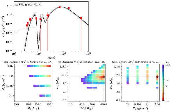
By minimizing the function defined in Eq. 4 of Zhang & Tan (2018) for each physical model, we find that the best five models are consistent with a ranging from 320 to 480 , a with 1.0-3.16 , and, most importantly, a current protostellar mass of (Table 5). The intrinsic bolometric luminosity is also a few L⊙, i.e., which is the level associated with such massive protostars. This further supports the findings from the P-V analysis from the molecular emission. Figure 13 panel a shows the best five models, with the best model represented with thick black line, and the observations as red squares. The error bars are set to be the larger of either 10% of the clump background-subtracted flux density to account for calibration error, or the value of the estimated clump background flux density. Note that all data points below are treated as upper limits (see, e.g., De Buizer et al., 2017). Panels (b) and (c) of Figure 13 show the 2D distribution of the three main physical parameters, i.e., , , and .
| Wavelength | Flux density |
|---|---|
| (µm) | (Jy) |
| Spitzer | |
| 3.6 | 0.02 (0.13) |
| 4.5 | 0.20 (0.33) |
| 8.0 | 0.58 (4.13) |
| 24.0 | 6.81 (12.00) |
| WISE | |
| 3.4 | 0.01 (0.08) |
| 4.6 | 0.27 (0.43) |
| 11.5 | 0.49 (5.31) |
| 22.0 | 6.92 (30.06) |
| Herschel | |
| 70.0 | 1352.47 (1539.58) |
| 160.0 | 2046.43 (2487.86) |
| 500.0 | 43.32 (86.73) |
Note. — Values in parenthesis are fluxes without the continuum subtraction. The photometric aperture radius was fixed at 16″, which was based on the m Herschel image.
| () | () | () | () | (∘) | () | () | (∘) | () | () | () | |
|---|---|---|---|---|---|---|---|---|---|---|---|
| 1.11 | 480 | 3.160 | 0.09 | 24 | 13 | 361.92 | 440.54 | 12 | 2.0 | 1.1 | 2.9 |
| 1.38 | 400 | 3.160 | 0.08 | 24 | 13 | 350.15 | 361.65 | 13 | 1.9 | 1.3 | 3.0 |
| 1.93 | 320 | 3.160 | 0.07 | 24 | 13 | 325.19 | 276.82 | 15 | 1.8 | 1.8 | 3.1 |
| 2.37 | 400 | 3.160 | 0.08 | 16 | 62 | 0.00 | 368.90 | 10 | 1.5 | 8.8 | 1.0 |
| 2.72 | 480 | 1.000 | 0.16 | 24 | 22 | 217.99 | 433.43 | 15 | 8.2 | 1.9 | 2.1 |
References
- Astropy Collaboration et al. (2013) Astropy Collaboration, Robitaille, T. P., Tollerud, E. J., et al. 2013, A&A, 558, A33. doi:10.1051/0004-6361/201322068
- Astropy Collaboration et al. (2018) Astropy Collaboration, Price-Whelan, A. M., Sipőcz, B. M., et al. 2018, AJ, 156, 123. doi:10.3847/1538-3881/aabc4f
- Bally et al. (2020) Bally, J., Ginsburg, A., Forbrich, J., et al. 2020, ApJ, 889, 178. doi:10.3847/1538-4357/ab65f2
- Bergner et al. (2018) Bergner, J. B., Guzmán, V. G., Öberg, K. I., et al. 2018, ApJ, 857, 69. doi:10.3847/1538-4357/aab664
- Bonnell et al. (2001) Bonnell, I. A., Bate, M. R., Clarke, C. J., et al. 2001, MNRAS, 323, 785. doi:10.1046/j.1365-8711.2001.04270.x
- Bradley et al. (2020) Bradley, L., Sipőcz, B., Robitaille, T., et al. 2020, Zenodo
- Caselli & Ceccarelli (2012) Caselli, P. & Ceccarelli, C. 2012, A&A Rev., 20, 56. doi:10.1007/s00159-012-0056-x
- Cesaroni et al. (2019) Cesaroni, R., Beltrán, M. T., Moscadelli, L., et al. 2019, A&A, 624, A100. doi:10.1051/0004-6361/201834700
- Cesaroni et al. (2017) Cesaroni, R., Sánchez-Monge, Á., Beltrán, M. T., et al. 2017, A&A, 602, A59. doi:10.1051/0004-6361/201630184
- Cleeves et al. (2017) Cleeves, L. I., Bergin, E. A., Öberg, K. I., et al. 2017, ApJ, 843, L3. doi:10.3847/2041-8213/aa76e2
- Crockett et al. (2014) Crockett, N. R., Bergin, E. A., Neill, J. L., et al. 2014, ApJ, 787, 112. doi:10.1088/0004-637X/787/2/112
- Csengeri et al. (2018) Csengeri, T., Bontemps, S., Wyrowski, F., et al. 2018, A&A, 617, A89. doi:10.1051/0004-6361/201832753
- De Buizer et al. (2017) De Buizer, J. M., Liu, M., Tan, J. C., et al. 2017, ApJ, 843, 33. doi:10.3847/1538-4357/aa74c8
- Gadhi et al. (1995) Gadhi, J., Lahrouni, A., Legrand, J., et al. 1995, Journal de Chimie Physique, 92, 1984. doi:10.1051/jcp/1995921984
- Goldsmith & Langer (1999) Goldsmith, P. F. & Langer, W. D. 1999, ApJ, 517, 209. doi:10.1086/307195
- Ilee et al. (2016) Ilee, J. D., Cyganowski, C. J., Nazari, P., et al. 2016, MNRAS, 462, 4386. doi:10.1093/mnras/stw1912
- Ilee et al. (2021) Ilee, J. D., Walsh, C., Booth, A. S., et al. 2021, ApJS, 257, 9. doi:10.3847/1538-4365/ac1441
- Johnston et al. (2015) Johnston, K. G., Robitaille, T. P., Beuther, H., et al. 2015, ApJ, 813, L19. doi:10.1088/2041-8205/813/1/L19
- Jørgensen et al. (2020) Jørgensen, J. K., Belloche, A., & Garrod, R. T. 2020, ARA&A, 58, 727. doi:10.1146/annurev-astro-032620-021927
- Le Gal et al. (2019) Le Gal, R., Brady, M. T., Öberg, K. I., et al. 2019, ApJ, 886, 86. doi:10.3847/1538-4357/ab4ad9
- Liu et al. (2019) Liu, M., Tan, J. C., De Buizer, J. M., et al. 2019, ApJ, 874, 16. doi:10.3847/1538-4357/ab07b7
- Liu et al. (2020) Liu, M., Tan, J. C., De Buizer, J. M., et al. 2020, ApJ, 904, 75. doi:10.3847/1538-4357/abbefb
- Loomis et al. (2018) Loomis, R. A., Cleeves, L. I., Öberg, K. I., et al. 2018, ApJ, 859, 131. doi:10.3847/1538-4357/aac169
- Maud et al. (2018) Maud, L. T., Cesaroni, R., Kumar, M. S. N., et al. 2018, A&A, 620, A31. doi:10.1051/0004-6361/201833908
- McKee & Tan (2002) McKee, C. F. & Tan, J. C. 2002, Nature, 416, 59. doi:10.1038/416059a
- McKee & Tan (2003) McKee, C. F. & Tan, J. C. 2003, ApJ, 585, 850. doi:10.1086/346149
- McMullin et al. (2007) McMullin, J. P., Waters, B., Schiebel, D., et al. 2007, Astronomical Data Analysis Software and Systems XVI, 376, 127
- Moscadelli et al. (2021) Moscadelli, L., Cesaroni, R., Beltrán, M. T., et al. 2021, A&A, 650, A142. doi:10.1051/0004-6361/202140829
- Moscadelli et al. (2018) Moscadelli, L., Rivilla, V. M., Cesaroni, R., et al. 2018, A&A, 616, A66. doi:10.1051/0004-6361/201832680
- Müller et al. (2005) Müller, H. S. P., Schlöder, F., Stutzki, J., et al. 2005, Journal of Molecular Structure, 742, 215. doi:10.1016/j.molstruc.2005.01.027
- Öberg et al. (2021) Öberg, K. I., Guzmán, V. V., Walsh, C., et al. 2021, ApJS, 257, 1. doi:10.3847/1538-4365/ac1432
- Pickett et al. (1998) Pickett, H. M., Poynter, R. L., Cohen, E. A., et al. 1998, J. Quant. Spec. Radiat. Transf., 60, 883. doi:10.1016/S0022-4073(98)00091-0
- Sánchez-Monge et al. (2013) Sánchez-Monge, Á., Cesaroni, R., Beltrán, M. T., et al. 2013, A&A, 552, L10. doi:10.1051/0004-6361/201321134
- Sakai et al. (2014) Sakai, N., Sakai, T., Hirota, T., et al. 2014, Nature, 507, 78. doi:10.1038/nature13000
- Sanna et al. (2021) Sanna, A., Giannetti, A., Bonfand, M., et al. 2021, arXiv:2107.05683
- Tan et al. (2014) Tan, J. C., Beltrán, M. T., Caselli, P., et al. 2014, Protostars and Planets VI, 149. doi:10.2458/azu_uapress_9780816531240-ch007
- Tanaka et al. (2016) Tanaka, K. E. I., Tan, J. C., & Zhang, Y. 2016, ApJ, 818, 52. doi:10.3847/0004-637X/818/1/52
- Tanaka et al. (2017) Tanaka, K. E. I., Tan, J. C., & Zhang, Y. 2017, ApJ, 835, 32. doi:10.3847/1538-4357/835/1/32
- Tanaka et al. (2020) Tanaka, K. E. I., Zhang, Y., Hirota, T., et al. 2020, ApJ, 900, L2. doi:10.3847/2041-8213/abadfc
- Taniguchi et al. (2020) Taniguchi, K., Guzmán, A. E., Majumdar, L., et al. 2020, ApJ, 898, 54. doi:10.3847/1538-4357/ab994d
- Taniguchi et al. (2019a) Taniguchi, K., Herbst, E., Caselli, P., et al. 2019a, ApJ, 881, 57. doi:10.3847/1538-4357/ab2d9e
- Taniguchi et al. (2021a) Taniguchi, K., Herbst, E., Majumdar, L., et al. 2021a, ApJ, 908, 100. doi:10.3847/1538-4357/abd6c9
- Taniguchi et al. (2021b) Taniguchi, K., Majumdar, L., Takakuwa, S., et al. 2021b, ApJ, 910, 141. doi:10.3847/1538-4357/abe854
- Taniguchi et al. (2017) Taniguchi, K., Ozeki, H., & Saito, M. 2017, ApJ, 846, 46. doi:10.3847/1538-4357/aa82ba
- Taniguchi et al. (2016) Taniguchi, K., Saito, M., & Ozeki, H. 2016, ApJ, 830, 106. doi:10.3847/0004-637X/830/2/106
- Taniguchi et al. (2019b) Taniguchi, K., Saito, M., Sridharan, T. K., et al. 2019b, ApJ, 872, 154. doi:10.3847/1538-4357/ab001e
- Wang et al. (2010) Wang, P., Li, Z.-Y., Abel, T., et al. 2010, ApJ, 709, 27. doi:10.1088/0004-637X/709/1/27
- Wright et al. (2020) Wright, M., Plambeck, R., Hirota, T., et al. 2020, ApJ, 889, 155. doi:10.3847/1538-4357/ab5864
- Wyrowski et al. (1999) Wyrowski, F., Schilke, P., & Walmsley, C. M. 1999, A&A, 341, 882
- Zhang & Tan (2018) Zhang, Y. & Tan, J. C. 2018, ApJ, 853, 18. doi:10.3847/1538-4357/aaa24a
- Zhang et al. (2019a) Zhang, Y., Tan, J. C., Sakai, N., et al. 2019a, ApJ, 873, 73. doi:10.3847/1538-4357/ab0553
- Zhang et al. (2019b) Zhang, Y., Tan, J. C., Tanaka, K. E. I., et al. 2019b, Nature Astronomy, 3, 517. doi:10.1038/s41550-019-0718-y
- Zhang et al. (2019c) Zhang, Y., Tanaka, K. E. I., Rosero, V., et al. 2019c, ApJ, 886, L4. doi:10.3847/2041-8213/ab5309