VideoSet
VideoSet: A Large-Scale Compressed Video Quality Dataset Based on JND Measurement
Abstract
A new methodology to measure coded image/video quality using the just-noticeable-difference (JND) idea was proposed in [1]. Several small JND-based image/video quality datasets were released by the Media Communications Lab at the University of Southern California in [2, 3]. In this work, we present an effort to build a large-scale JND-based coded video quality dataset. The dataset consists of 220 5-second sequences in four resolutions (i.e., , , and ). For each of the 880 video clips, we encode it using the H.264 codec with and measure the first three JND points with 30+ subjects. The dataset is called the ‘VideoSet’, which is an acronym for ‘Video Subject Evaluation Test (SET)’. This work describes the subjective test procedure, detection and removal of outlying measured data, and the properties of collected JND data. Finally, the significance and implications of the VideoSet to future video coding research and standardization efforts are pointed out. All source/coded video clips as well as measured JND data included in the VideoSet are available to the public in the IEEE DataPort [4].
1 Introduction
Digital video plays an important role in our daily life. About 70% of today’s Internet traffic is attributed to video, and it will continue to grow to the 80-90% range within a couple of years. It is critical to have a major breakthrough in video coding technology to accommodate the rapid growth of video traffic. Despite the introduction of a set of fine-tuned coding tools in the standardization of H.264/AVC and H.265 (or HEVC), a major breakthrough in video coding technology is needed to meet the practical demand. To address this problem, we need to examine limitations of today’s video coding methodology.
Today’s video coding technology is based on Shannon’s source coding theorem, where a continuous and convex rate-distortion (R-D) function for a probabilistic source is derived and exploited (see the black curve in Fig. 1). However, humans cannot perceive small variation in pixel differences. Psychophysics study on the just-noticeable difference (JND) clearly demonstrated the nonlinear relation between human perception and physical changes. The traditional R-D function does not take this nonlinear human perception process into account. In the context of image/video coding, recent subjective studies in [1] show that humans can only perceive discrete-scale distortion levels over a wide range of coding bitrates (see the red curve in Fig. 1).
Without loss of generality, we use H.264 video as an example to explain it. The quantization parameter (QP) is used to control its quality. The smaller the QP, the better the quality. Although one can choose a wide range of QP values, humans can only differentiate a small number of discrete distortion levels among them. In contrast with the conventional R-D function, the perceived R-D curve is neither continuous nor convex. Rather, it is a stair function that contains a couple of jump points, called just noticeable difference (JND) points. The JND is a statistical quantity that accounts for the maximum difference unnoticeable to a human being. Subjective tests for traditional visual coding and processing were only conducted by very few experts called golden eyes. This is the worst-case analysis. As the emergence of big data science and engineering, the worst-case analysis cannot reflect the statistical behavior of the group-based quality of experience (QoE). When the subjective test is conducted with respect to a viewer group, it is more meaningful to study their QoE statistically to yield an aggregated function.
 \phantomcaption
The measure of coded image/video quality using the JND notion was first proposed in [1]. As a follow-up, two small-scale JND-based image/video quality datasets were released by the Media Communications Lab at the University of Southern California. They are the MCL-JCI dataset [2] and the MCL-JCV dataset [3] targeted the JPEG image and the H.264 video, respectively. To build a large-scale JND-based video quality dataset, an alliance of academic and industrial organizations was formed and the subjective test data were acquired in Fall 2016. The resulting dataset is called the “VideoSet” – an acronym for “Video Subject Evaluation Test (SET)”. The VideoSet consists of 220 5-second sequences in four resolutions (i.e., , , and ). For each of the 880 video clips, we encode it using the x264 [5] encoder implementation of the H.264 standard with and measure the first three JND points with 30+ subjects. All source/coded video clips as well as measured JND data included in the VideoSet are available to the public in the IEEE DataPort [4].
The rest of this paper is organized as follows. The source and compressed video content preparation is discussed in Sec. 2. The subjective evaluation procedure is described in Sec. 3. The outlier detection and removal process is conducted for JND data post-processing in Sec. 4. Some general discussion on the VideoSet is provided in Sec. 5. The significance and implication of the VideoSet to future video coding research and standardization efforts are pointed out in Sec. 6. Finally, concluding remarks and future work are given in Sec. 7.
2 Source and Compressed Video Content
We describe both the source and the compressed video content in this section.
2.1 Source Video
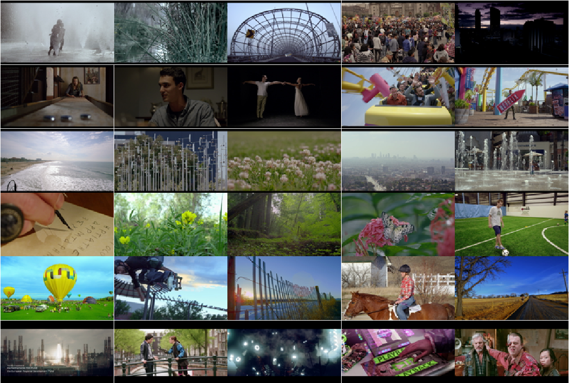
The VideoSet consists of 220 source video clips, each of which has a duration of 5 seconds. We show thumbnails images for 30 representative video clips in Fig 2. The source video clips were collected from publicly available datasets in [6, 7, 8]. The original sequences have multiple spatial resolutions (i.e., , , ), frame rates (i.e., 60, 30, 24) and color formats (i.e., YUV444p, YUV422p, YUV420p). We pay special attention to the selection of these source video clips to avoid redundancy and enrich diversity of selected contents.
After content selection, we process each 5-second video clip to ensure that they are in similar format. Their formats are summarized in Table 1, where the first column shows the names of the source video material of longer duration and the second column indicates the number of video clips selected from each source material. The third, fourth and fifth columns describe the frame rate, the spatial resolution and the pixel format, respectively. They are further explained below.
-
•
Frame Rate. The frame rate affects the perceptual quality of certain contents significantly [9]. Contents of a higher frame rate (e.g. 60fps) demand a more powerful CPU and a larger memory to avoid impairments in playback. For this reason, if the original frame rate is 60fps, we convert it from 60fps to 30fps to ensure smooth playback in a typical environment. If the original frame rate is not greater than 30fps, no frame rate conversion is needed.
-
•
Spatial Resolution. The aspect ratio of most commonly used display resolutions for web users is . For inconsistent aspect ratios, we scale them to by padding black horizontal bars above and below the active video window. As a result, all video clips are of the same spatial resolution – .
-
•
Pixel Format. We down-sample the trimmed spatial resolution (2160p) to four lower resolutions. They are: (1080p), (720p), (540p) and (360p) for the subjective test in building the VideoSet. In the spatial down-sampling process, the lanczos interpolation [10] is used to keep a good compromise between low and high frequencies components. Also, the chroma sampling is adopted for maximum compatibility.
It is worthwhile to point out that 1080p and 720p are two most dominant video formats on the web nowadays while 540p and 360p are included to capture the viewing experience on tablets or mobile phones. After the above-mentioned processing, we obtain 880 uncompressed sequences in total.
| Frame rate | Spatial resolution | Pixel format | |||||
|---|---|---|---|---|---|---|---|
| Source | Selected | Original | Trimmed | Original | Trimmed | Original | Trimmed |
| El Fuente | 31 | 60 | 30 | YUV444p | YUV420p | ||
| Chimera | 59 | 30 | 30 | YUV422p | YUV420p | ||
| Ancient Thought | 11 | 24 | 24 | YUV422p | YUV420p | ||
| Eldorado | 14 | 24 | 24 | YUV422p | YUV420p | ||
| Indoor Soccer | 5 | 24 | 24 | YUV422p | YUV420p | ||
| Life Untouched | 15 | 60 | 30 | YUV444p | YUV420p | ||
| Lifting Off | 13 | 24 | 24 | YUV422p | YUV420p | ||
| Moment of Intensity | 10 | 60 | 30 | YUV422p | YUV420p | ||
| Skateboarding | 9 | 24 | 24 | YUV422p | YUV420p | ||
| Unspoken Friend | 13 | 24 | 24 | YUV422p | YUV420p | ||
| Tears of Steel | 40 | 24 | 24 | YUV420p | YUV420p | ||
2.2 Video Encoding
We use the H.264/AVC [5] high profile to encode each of the 880 sequences, and choose the constant quantization parameter (CQP) as the primary bit rate control method. The adaptive QP adjustment is reduced to the minimum amount since our primary goal is to understand a direct relationship between the quantization parameter and perceptual quality. The encoding recipe is included in the read-me file of the released dataset.
The QP values under our close inspection are between . It is unlikely to observe any perceptual difference between the source and coded clips with a QP value smaller than . Furthermore, coded video clips with a QP value larger than will not be able to offer acceptable quality. On the other hand, it is ideal to examine the full QP range; namely, , in the subjective test since the JND measure is dependent on the anchor video that serves as a fixed reference.
To find a practical solution, we adopt the following modified scheme. The reference is losslessly encoded and referred to as . We use the source to substitute all sequences with a QP value smaller than 8. Similarly, sequences with a QP larger value than 47 are substituted by that with . The modification has no influence on the subjective test result. This will become transparent when we describe the JND search procedure in Sec. 3.2. By including the source and all coded video clips, there are video clips in the VideoSet.
3 Subjective Test Environment and Procedure
The subjective test environment and procedure are described in detail in this section.
3.1 Subjective Test Environment
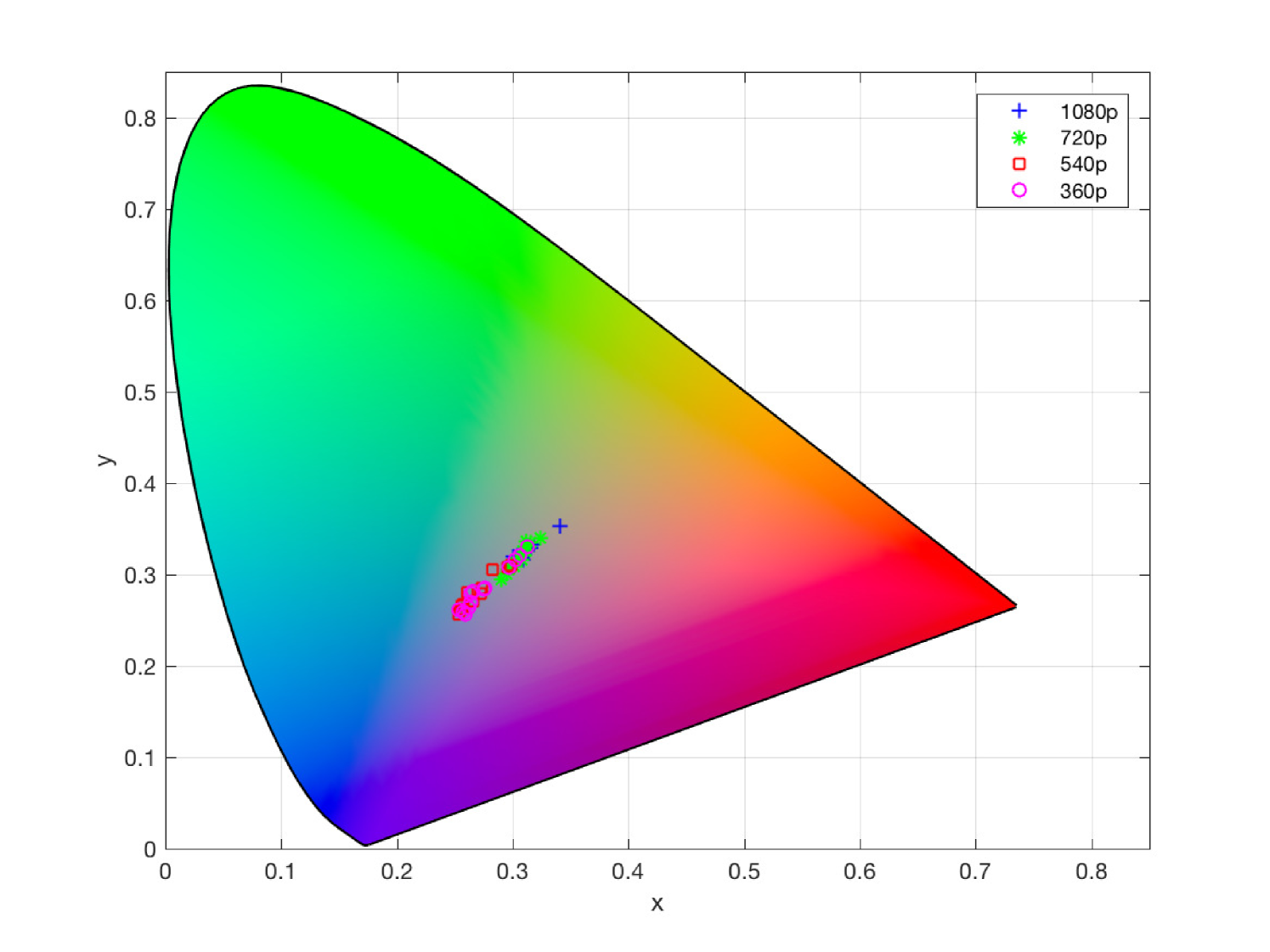
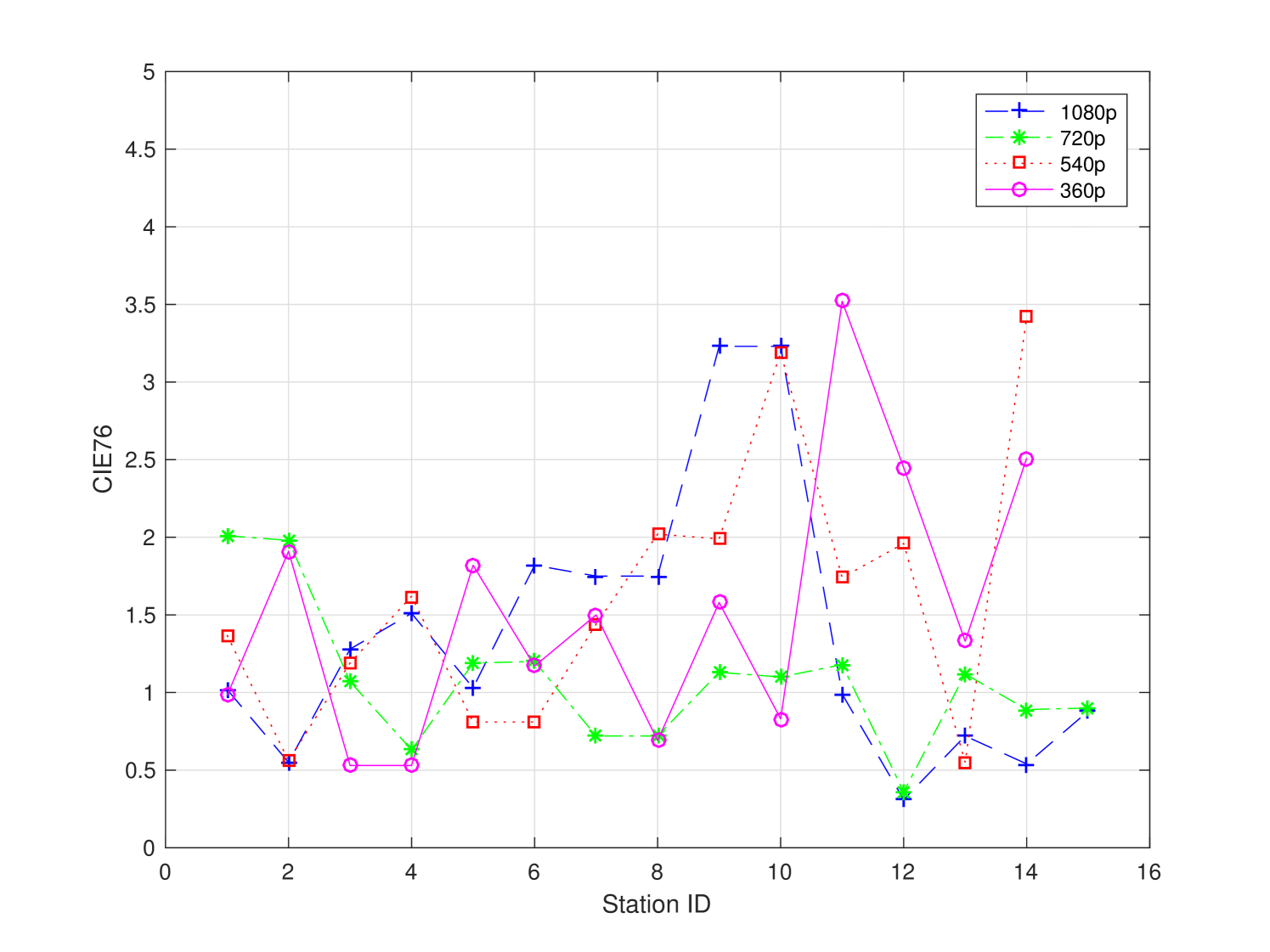
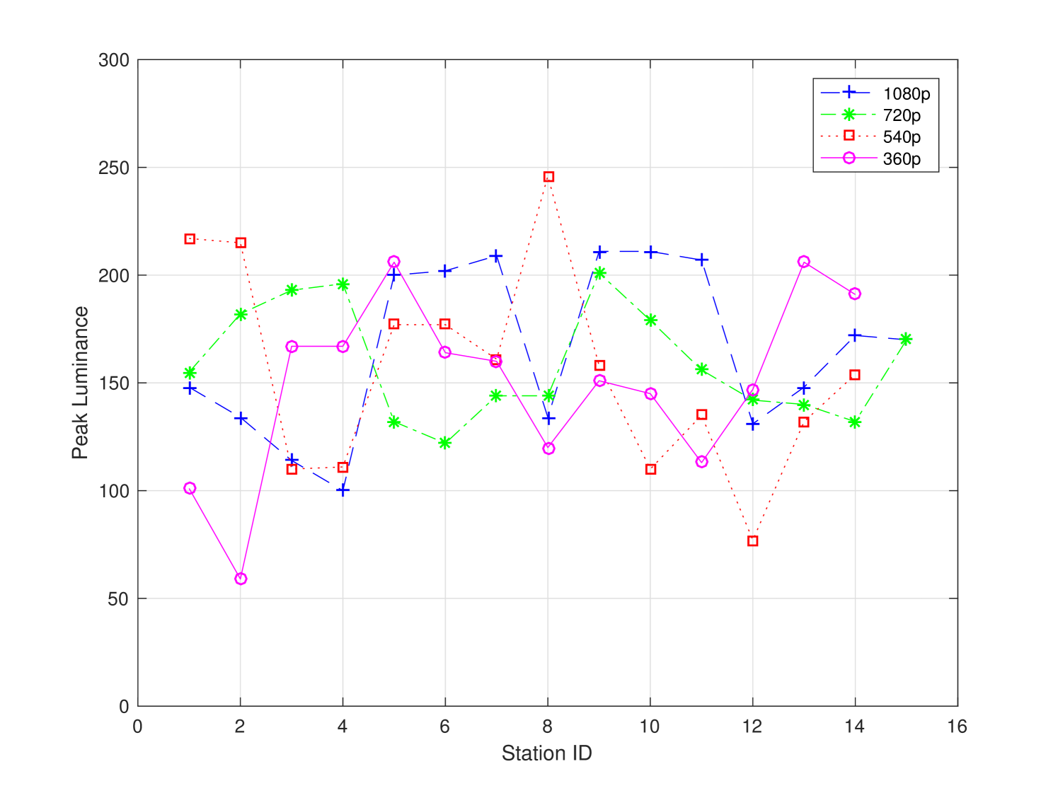
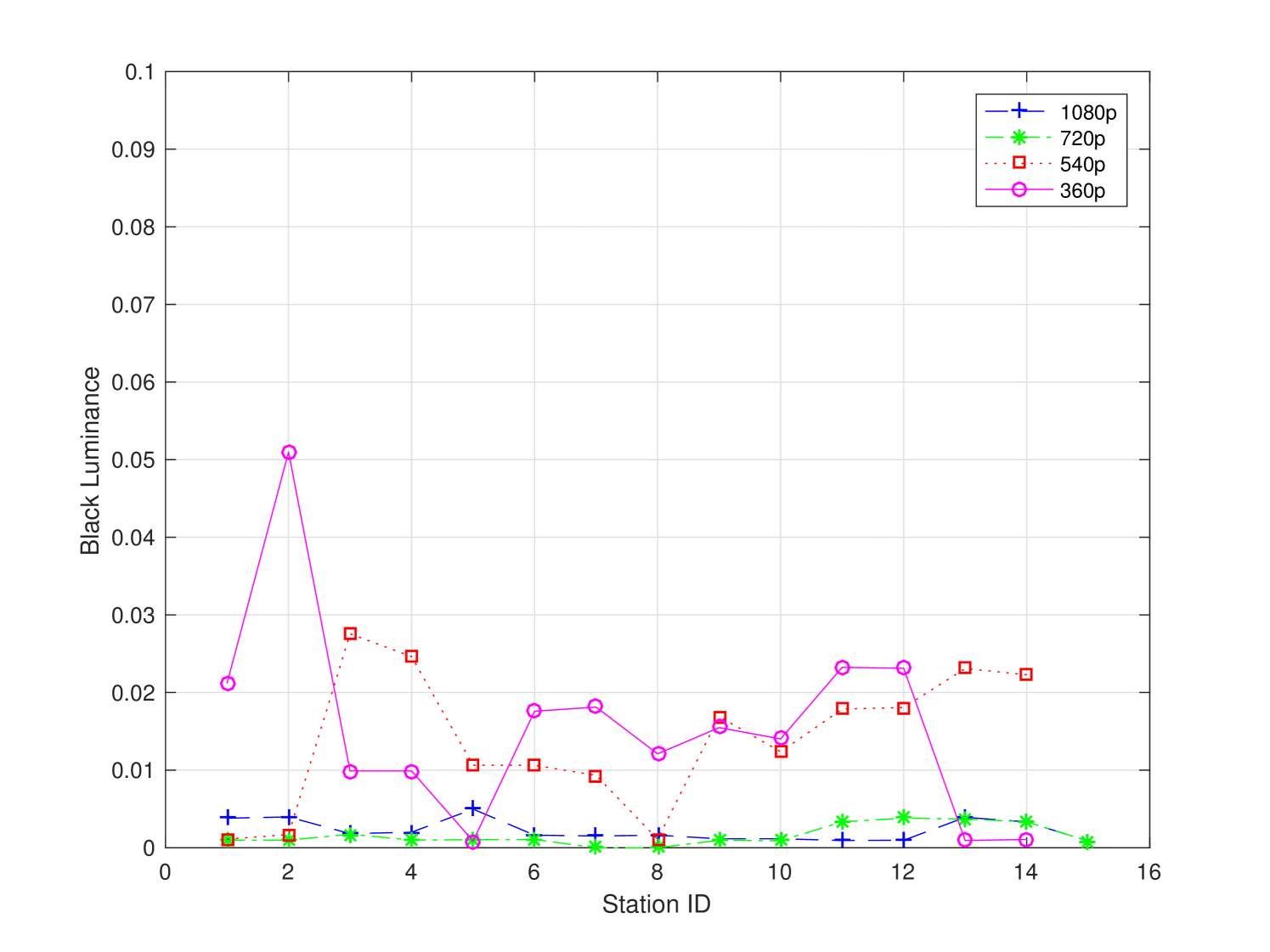
The subjective test was conducted in six universities in the city of Shenzhen in China. There were 58 stations dedicated to the subjective test. Each station offered a controlled non-distracting laboratory environment. The viewing distance was set as recommended in ITU-R BT.2022. The background chromaticity and luminance were set up as an environment of a common office/laboratory. We did not conduct monitor calibration among different test stations, yet the monitors were adjusted to a comfortable setting to test subjects. On one hand, the uncalibrated monitors provided a natural platform to capture the practical viewing experience in our daily life. On the other hand, the monitors used in the subjective test were profiled for completeness. Monitor profiling results are given in Fig. 3 and summarized in Table 2. As shown in Table 2, most stations comply with ITU recommendations.
We indexed each video clip with a content ID and a resolution ID and partitioned 880 video clips into 58 packages. Each package contains 14 or 15 sequence sets of a content/resolution ID pair, and each sequence set contains one source video clip and its all coded video clips. One subject can complete one JND point search for one package in one test session. The duration of one test session was around 35 minutes with a 5-minute break in the middle. Video sequences were displayed in their native resolution without scaling on the monitor. The color of the inactive screen was set to light gray.
We randomly recruited around 800 students to participate in the subjective test. A brief training session was given to each subject before a test session starts. In the training session, we used different video clips to show quality degradation of coded video contents. The scenario of our intended application; namely, the daily video streaming experience, was explained. Any question from the subject about the subjective test was also answered.
| Resolution | Station Number | Peak Luminance () | Black Luminance | Color Difference | Viewing Distance () |
|---|---|---|---|---|---|
| 1080p | |||||
| 720p | |||||
| 540p | |||||
| 360p |
3.2 Subjective Test Procedure
In the subjective test, each subject compares the quality of two clips displayed one after another, and determines whether these two sequences are noticeably different or not. The subject should choose either ‘YES’ or ‘NO’ to proceed. The subject has an option to ask to play the two sequences one more time. The comparison pair is updated based on the response.
One aggressive binary search procedure was described in [3] to speed up the JND search process. At the first comparison, the procedure asked a subject whether there would be any noticeable difference between and . If a subject made an unconfident decision of ‘YES’ at the first comparison, the test procedure would exclude interval in the next comparison. Although the subjects selects ‘Noticeable Difference’ in all comparisons afterwards, the final JND location would stay at . It could not belong to any longer. A similar problem arose if a subject made an unconfident decision of ‘NO’ at the first comparison.
To fix this problem, we adopt a more robust binary search procedure in our current subjective test. Instead of eliminating the entire left or right half interval, only one quarter of the original interval at the farthest location with respect to the region of interest is dropped in the new test procedure. Thus, if a subject made an unconfident decision of ‘YES’ at the first comparison, the test procedure will remove interval so that the updated interval is . The new binary search procedure allows a buffer even if a wrong decision is made. The comparison points may oscillate around the final JND position but still converge to it. The new binary search procedure is proved to be more robust than the previous binary search procedure at the cost of a slightly increased number of comparisons (i.e., from 6 comparisons in the previous procedure to 8 comparisons in the new procedure).
Let be the QP used to encode a source sequence. We use and as the start and the end QP values of a search interval, , at a certain round. Since , the quality of the coded video clip with is better than that with . We use to denote the QP value of the anchor video clip. It is fixed in the entire binary search procedure until the JND point is found. The QP value, , of the comparison video is updated within . One round of the binary search procedure is described in Algorithm 1.
The global JND search algorithm is stated below.
-
•
Initialization. We set and .
-
•
Search range update. If and exhibit a noticeable quality difference, update to the third quartile of the range. Otherwise, update to the first quartile of the range. The ceiling and the floor integer-rounded operations, denoted by and , are used in the update process as shown in the Algorithm of the one round of the JND search procedure.
-
•
Comparison video update. The QP value of the comparison video clip is set to the middle point of the range under evaluation with the integer-rounded operation.
-
•
Termination. There are two termination cases. First, if and the comparison result is ‘Noticeable Difference’, then search process is terminated and is set to the JND point. Second, if and the comparison result is ‘Unnoticeable Difference’, the process is terminated and the JND is the latest when the comparison result was ‘Noticeable Difference’.
The JND location depends on the characteristics of the underlying video content, the visual discriminant power of a subject and the viewing environment. Each JND point can be modeled as a random variable with respect to a group of test subjects. We search and report three JND points for each video clip in the VideoSet. It will be argued in Sec. 5 that the acquisition of three JND values are sufficient for practical applications.
For a coded video clip set, the same anchor video is used for all test subjects. The anchor video selection procedure is given below. We plot the histogram of the current JND point collected from all subjects and then set the QP value at its first quartile as the anchor video in the search of the next JND point. For this QP value, of test subjects cannot notice a difference. We select this value rather than the median value, where of test subjects cannot see a difference, so as to set up a higher bar for the next JND point. The first JND point search is conducted for QP belonging to . Let be the QP value of the JND point for a given sequence. The QP search range for JND is .
4 JND Data Post-Processing via Outlier Removal
Outliers refer to observations that are significantly different from the majority of other observations. The notation applies to both test subjects and collected samples. In practice, outliers should be eliminated to allow more reliable conclusion. For JND data post-processing, we adopt outlier detection and removal based on the individual subject and collected JND samples. They are described below.
4.1 Unreliable Subjects
As described in Sec. 2.2, video clips are encoded with while denotes the source video without any quality degradation. The QP range is further extended to by substituting video of with video of , and video of with video of . With this substitution, the video for is actually lossless, and no JND point should lie in this range. If a JND sample of a subject comes to this interval, the subject is treated as an outlier. All collected samples from this subject are removed.
The ITU-R BT 1788 document provides a statistical procedure on subject screening. It examines score consistency of a subject against all subjects in a test session, where the scores typically range from 1 to 5 denoting from the poorest to the best quality levels. This is achieved by evaluating the correlation coefficient between the scores of a particular subject with the mean scores of all subjects for the whole test session, where the Pearson correlation or the Spearman rank correlation is compared against a pre-selected threshold. However, this procedure does not apply to the collected JND data properly since our JND data is the QP value of the coded video that meets the just noticeable difference criterion.
Alternatively, we adopt the z-scores consistency check. Let be the samples obtained from subject on a video sequence set with video index , where and . For subject , we can form a vector of his/her associated samples as
| (1) |
Its mean and standard deviation (SD) vectors against all subjects can be written as
| (2) | |||||
| (3) |
Then, the z-scores vector of subject is defined as
| (4) |
The quantity, , indicates the distance between the raw score and the population mean in the SD unit for subject and video clip . The dispersion of the z-score vector shows consistency of an individual subject with respect to the majority.
Both the range and the SD of the z-score vector, , are used as the dispersion metrics. They are defined as
| (5) |
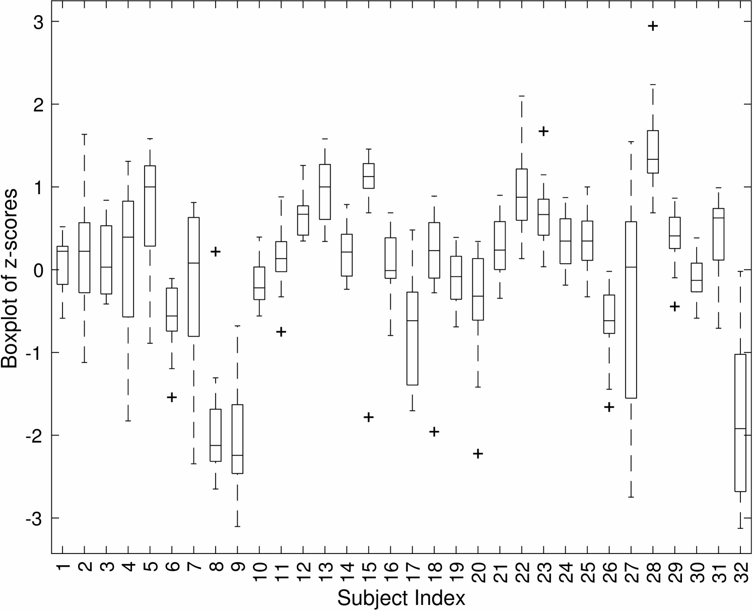
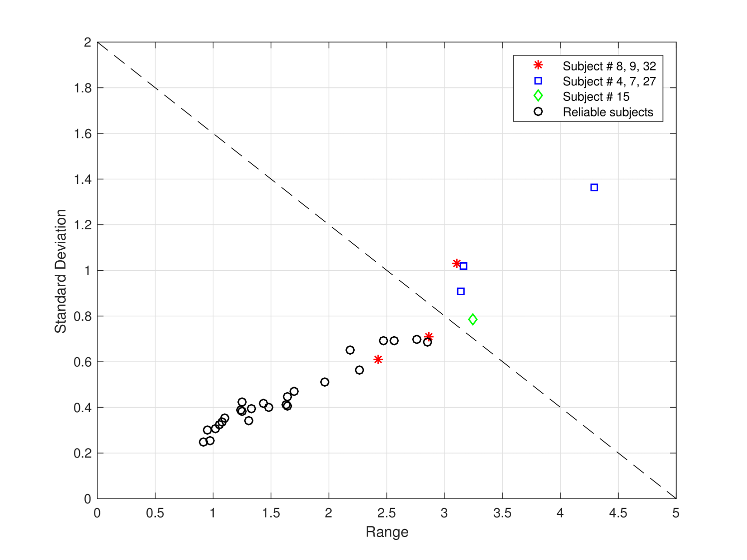
respectively. A larger dispersion indicates that the corresponding subject gives inconsistent evaluation results in the test. A subject is identified as an outlier if the associated range and SD values are both large. An example is shown in Fig. 4. We provide the boxplot of z-scores for all 32 subjects in Fig. 4(a) and the corresponding dispersion plot in Fig. 4(b). The horizontal and the vertical axes of Fig. 4(b) are the range and the SD metrics, respectively.
For this particular test example, subjects #8, #9 and #32 are detected as outliers because some of their JND samples have . Subjects #4, #7 and #27 are removed since their range and SD are both large. For subject #15, the SD value is small yet the range is large due to one sample. We remove that sample and keep others.
4.2 Outlying Samples
Besides unreliable subjects, we consider outlying samples for a given test content. This may be caused by the impact of the unique characteristics of different video contents on the perceived quality of an individual. Here, we use the Grubbs’ test [12] to detect and remove outliers. It detects one outlier at a time. If one sample is declared as an outlier, it is removed from the dataset, and the test is repeated until no outliers are detected.
We use to denote a set of raw samples collected for one test sequence. The test statistics is the largest absolute deviation of a sample from the sample mean in the SD unit. Mathematically, the test statistics can be expressed as
| (6) |
At a given significant level denoted by , a sample is declared as an outlier if
| (7) |
where is the upper critical value of the t-distribution with degrees of freedom. In our subjective test, the sample size is around after removing unreliable subjects and outlying samples. We set the significance level at as a common scientific practice. Then, a sample is identified as an outlier if its distance to the sample mean is larger than the SD unit.
4.3 Normality of Post-processed JND Samples
| Resolution | The first JND | The second JND | The third JND |
|---|---|---|---|
| 1080p | |||
| 720p | |||
| 540p | |||
| 360p |
Each JND point is a random variable. We would like to check whether it can be approximated by a Gaussian random variable [3] after outlier removal. The test was suggested in ITU-R BT.500 to test whether a collected set of samples is normal or not. It calculates the kurtosis coefficient of the data samples and asserts that the distribution is Gaussian if the kurtosis is between 2 and 4.
Here, we adopt the Jarque-Bera test [13] to conduct the normality test. It is a two-sided goodness-of-fit test for normality of observations with unknown parameters. Its test statistic is defined as
| (8) |
where is the sample size, is the sample skewness and is the sample kurtosis. The test rejects the null hypothesis if the statistic in Eq. (8) is larger than the precomputed critical value at a given significance level, . This critical value can be interpreted as the probability of rejecting the null hypothesis given that it is true.
We show the percentage of sequences passing normality test in Table 3. It is clear from the table that a great majority of JND points do follow the Gaussian distribution after the post-processing procedure.
5 Discussion
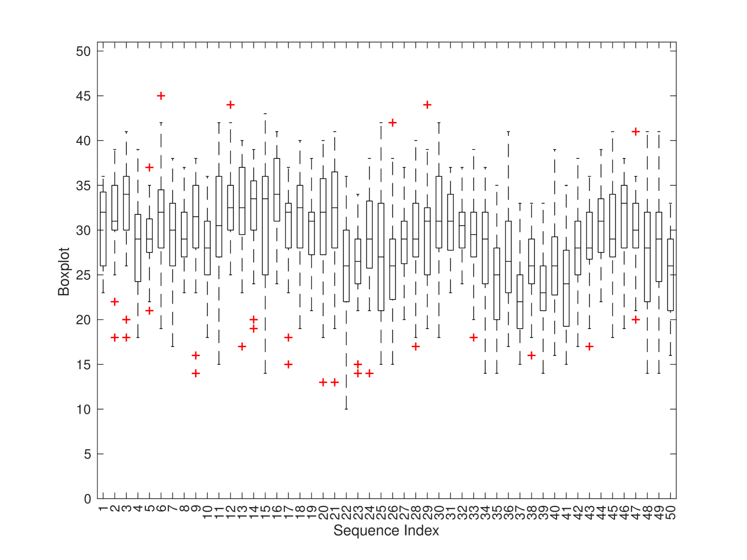
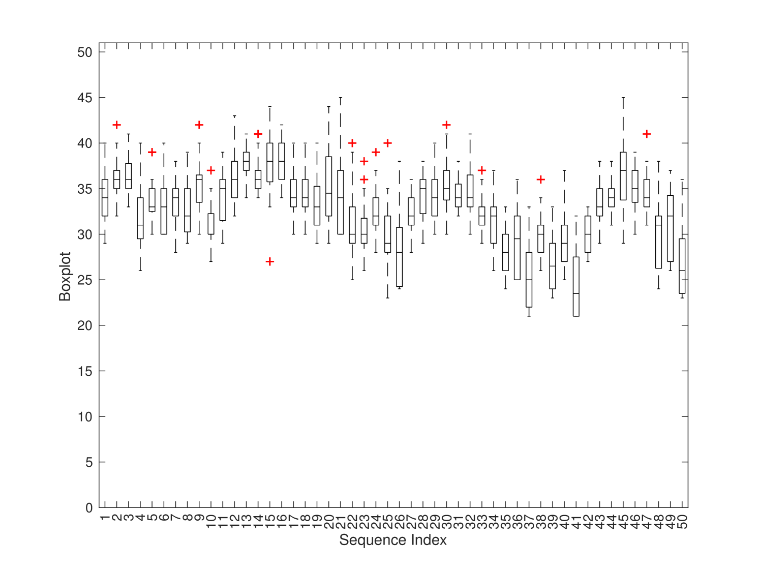
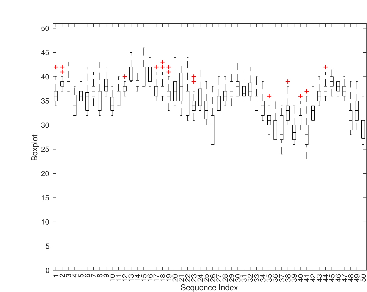
We show the JND distribution of the first 50 sequences (out of 220 sequences in total) with resolution 1080p in Fig. 5. The figure includes three sub-figures which show the distributions of the first, the second, and the third JND points, respectively. Generally speaking, there exhibit large variations among JND points across different sequences.
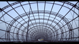
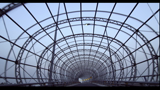
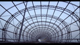
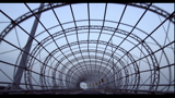

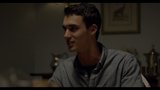
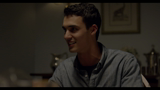
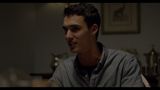
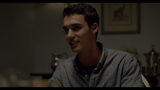
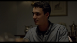
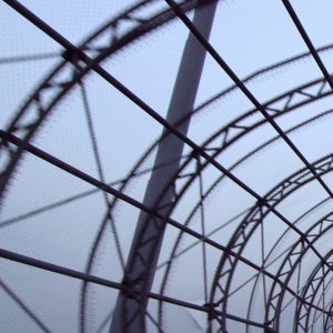
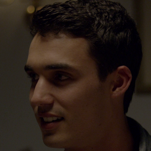
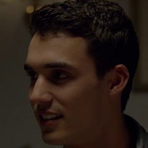
We examine sequences #15 (tunnel) and #37 (dinner) to offer deeper insights into the JND distribution. Representative frames are given in Fig. 6. Sequence #15 is a scene with fast motion and rapid background change. As a result, the masking effect is strong. It is not a surprise that the JND samples vary a lot among different subjects. As shown in Fig. 5(a), the JND samples of this sequence have the largest deviation among the 50 sequences in the plot. This property is clearly revealed by the collected JND samples. Sequence #37 is a scene captured around a dinner table. It focuses on a male speaker with dark background. The face of the man offers visual saliency that attracts the attention of most people. Thus, the quality variation of this sequence is more noticeable than others and its JND distribution is more compact. As shown in Fig. 5(a), sequence #37 has the smallest SD among the 50 sequences.
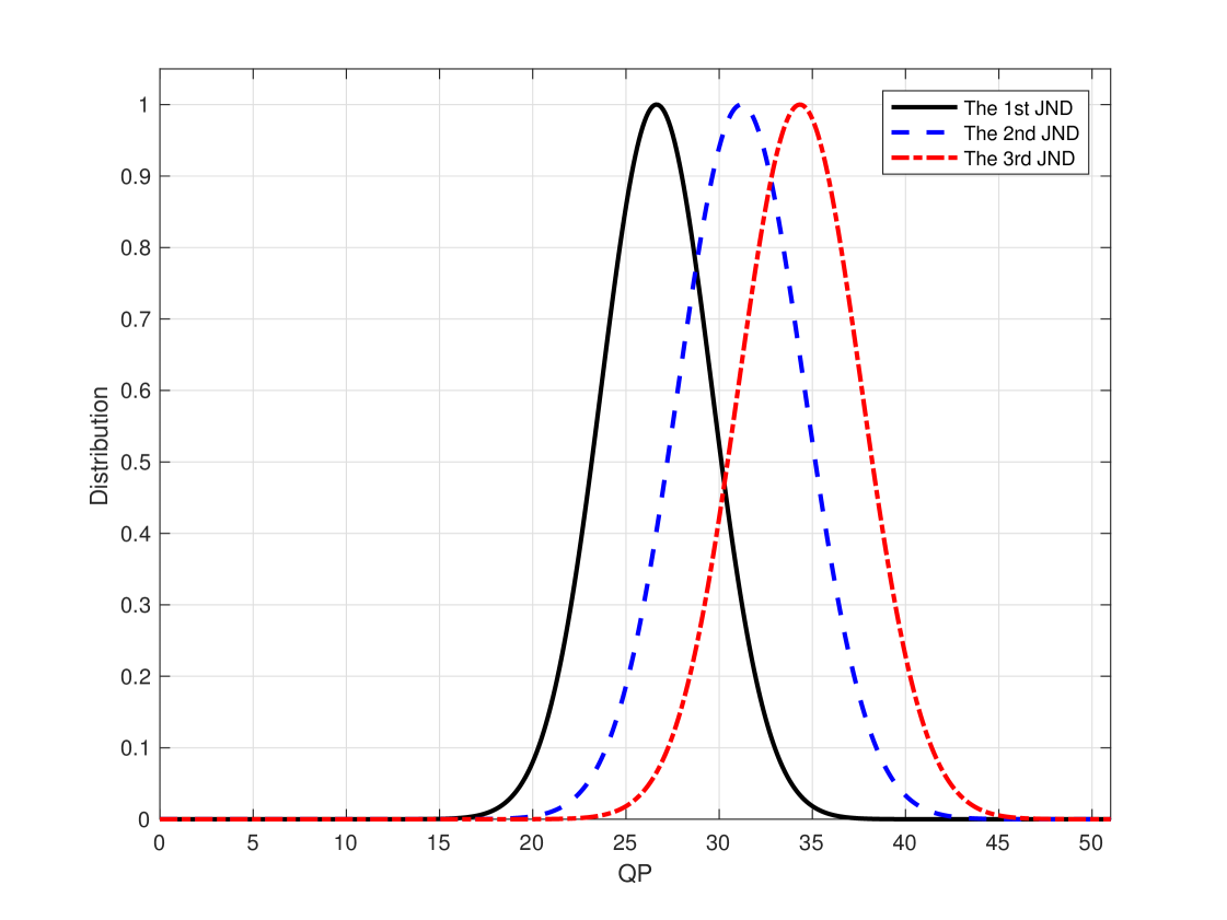
Furthermore, we plot the histograms of the first, the second, and the third JND points of all 220 sequences in Fig. 7. They are centered around QP = 27, 31 and 34, respectively. For the daily video service such as the over-the-top (OTT) content, the QP values are in the range of 18 to 35. Furthermore, take the traditional 5-level quality criteria as an example (i.e., excellent, good, fair, poor, bad). The quality of the third JND is between fair and poor. For these reasons, we argue that it is sufficient to measure 3 JND points. The quality of coded video clips that go beyond this range is too bad to be acceptable by today’s viewers in practical Internet video streaming scenarios.
 \phantomcaption
The scattered plots of the mean and the SD pairs of JND samples with four resolutions are shown in Fig. 8. We observe similar general trends of the scattered plots in Fig. 8 in all four resolutions. For example, the SD values of the second and the third JND points are significantly smaller than that of the first JND point. The first JND point, which is the boundary between the perceptually lossy and lossless coded video, is most difficult for subjects to determine. The main source of observed artifacts is slight blurriness. In contrast, subjects are more confident in the decision on the second and the third JND points. The dominant factor is noticeable blockiness.
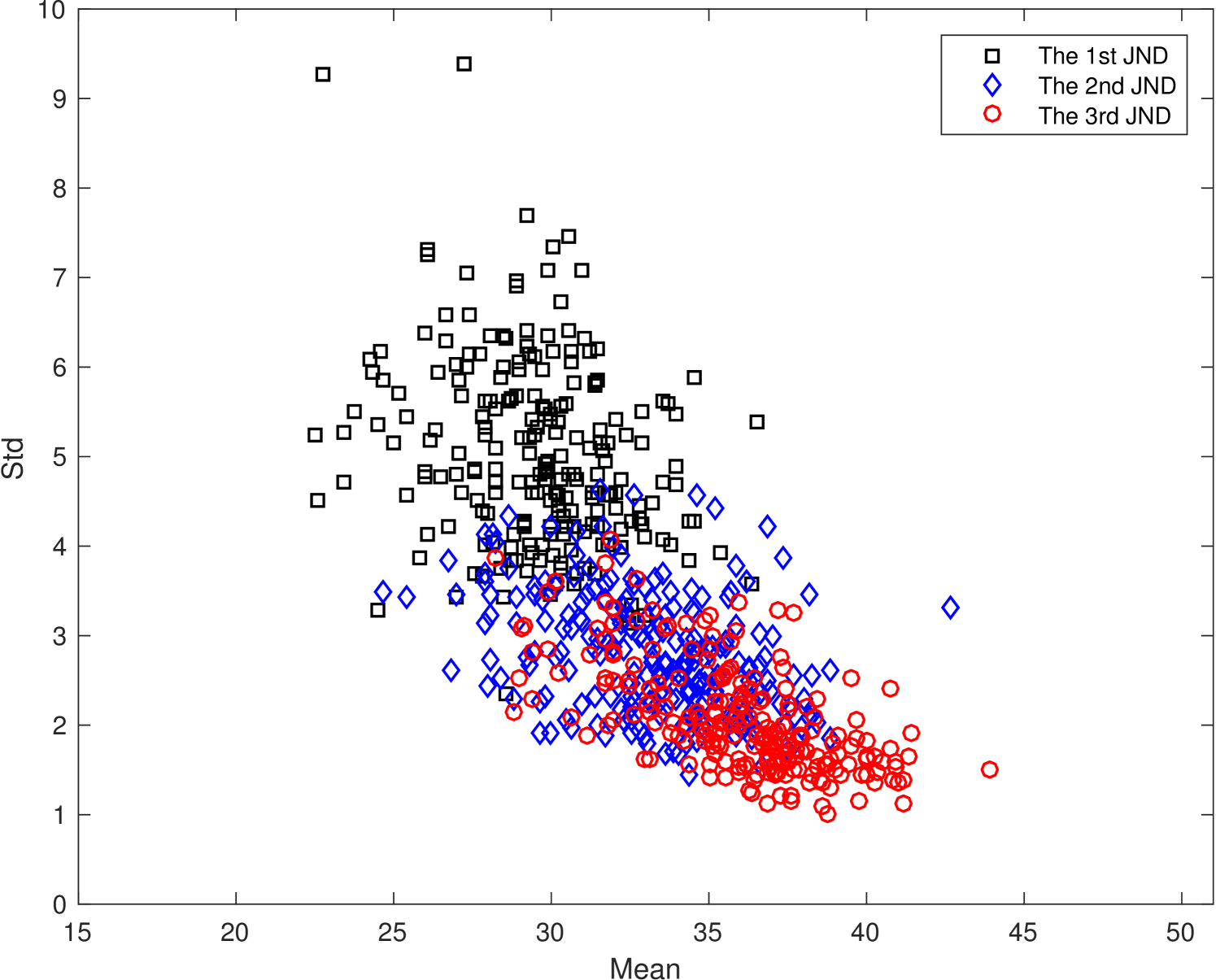
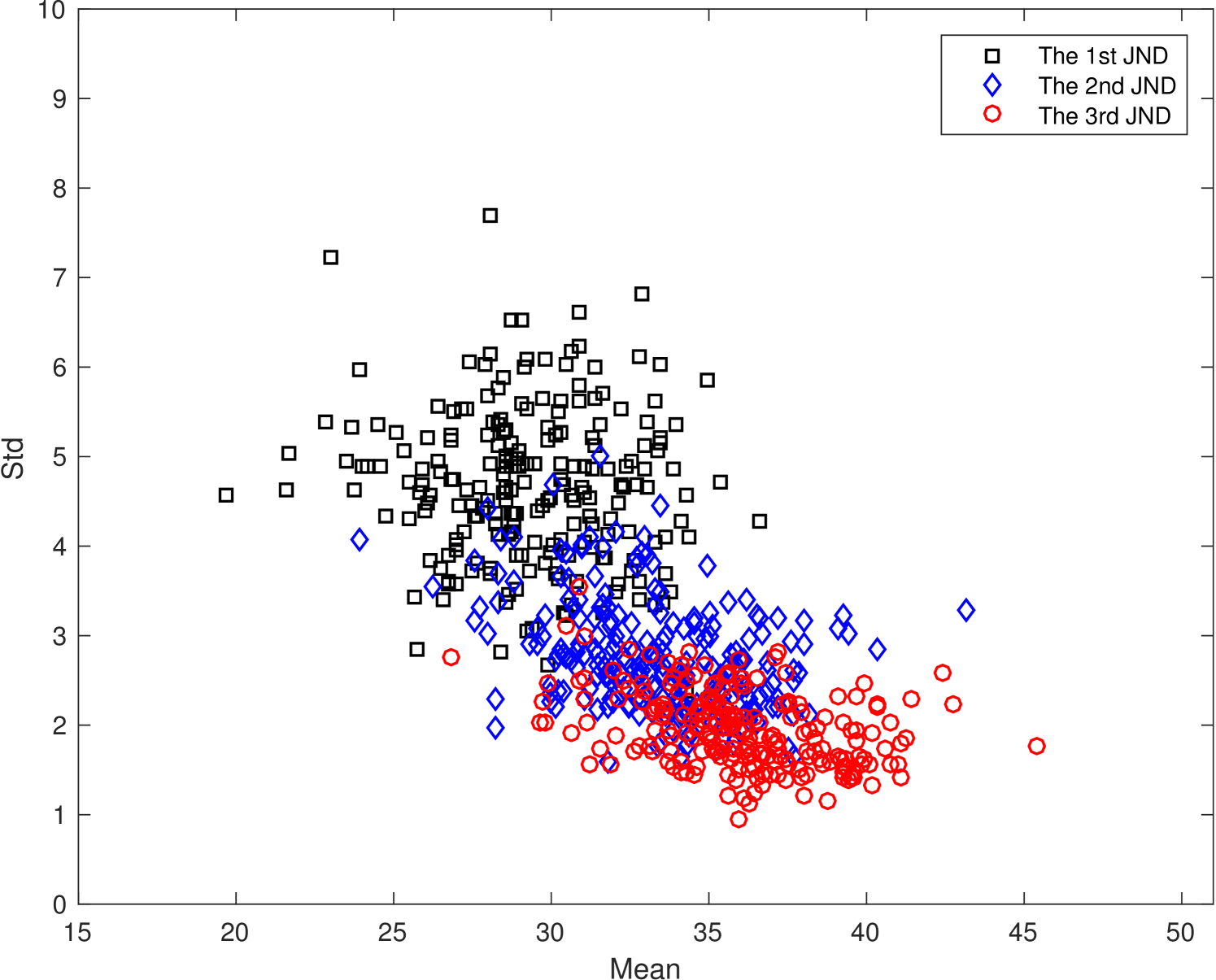
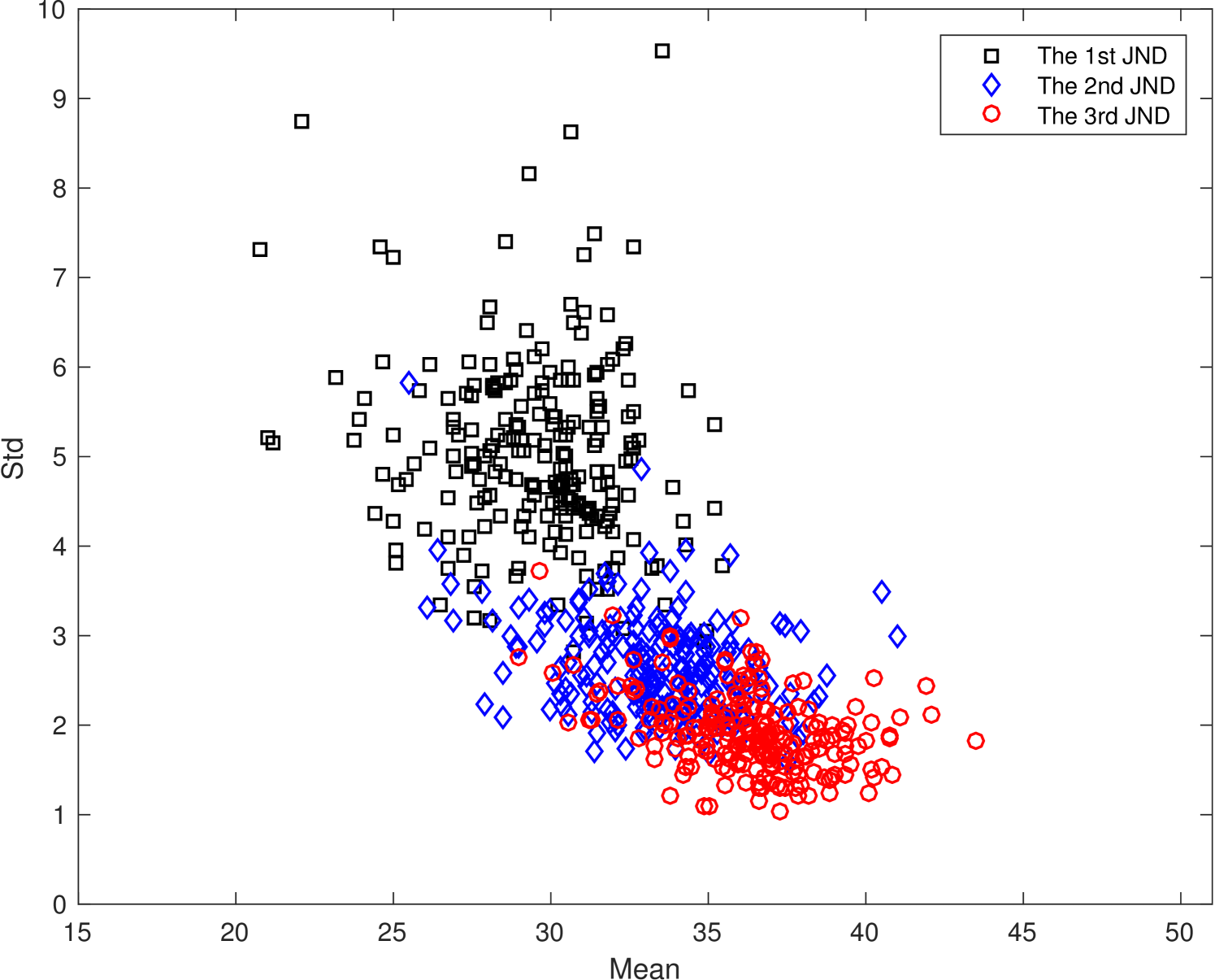
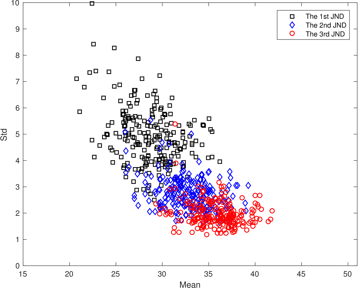
The masking effect plays an important role in the visibility of artifacts. For sequences with a large SD value such as sequence # 15 in Fig. 5(a), its masking effect is strong. On one hand, the JND arrives earlier for some people who are less affected by the masking effect so that they can see the compression artifact easily. On the other hand, the compression artifact is masked with respect to others so that the coding artifact is less visible. For the same reason, the masking effect is weaker for sequences with a smaller SD value.
6 Significance and Implications of VideoSet
The peak-signal-to-noise (PSNR) value has been used extensively in the video coding community as the video quality measure. Although it is easy to measure, it is not exactly correlated with the subjective human visual experience [14]. The JND measure demands a great amount of effort in conducting the subjective evaluation test. However, once a sufficient amount of data are collected, it is possible to use the machine learning technique to predict the JND value within a short interval. The construction of the VideoSet serves for this purpose.
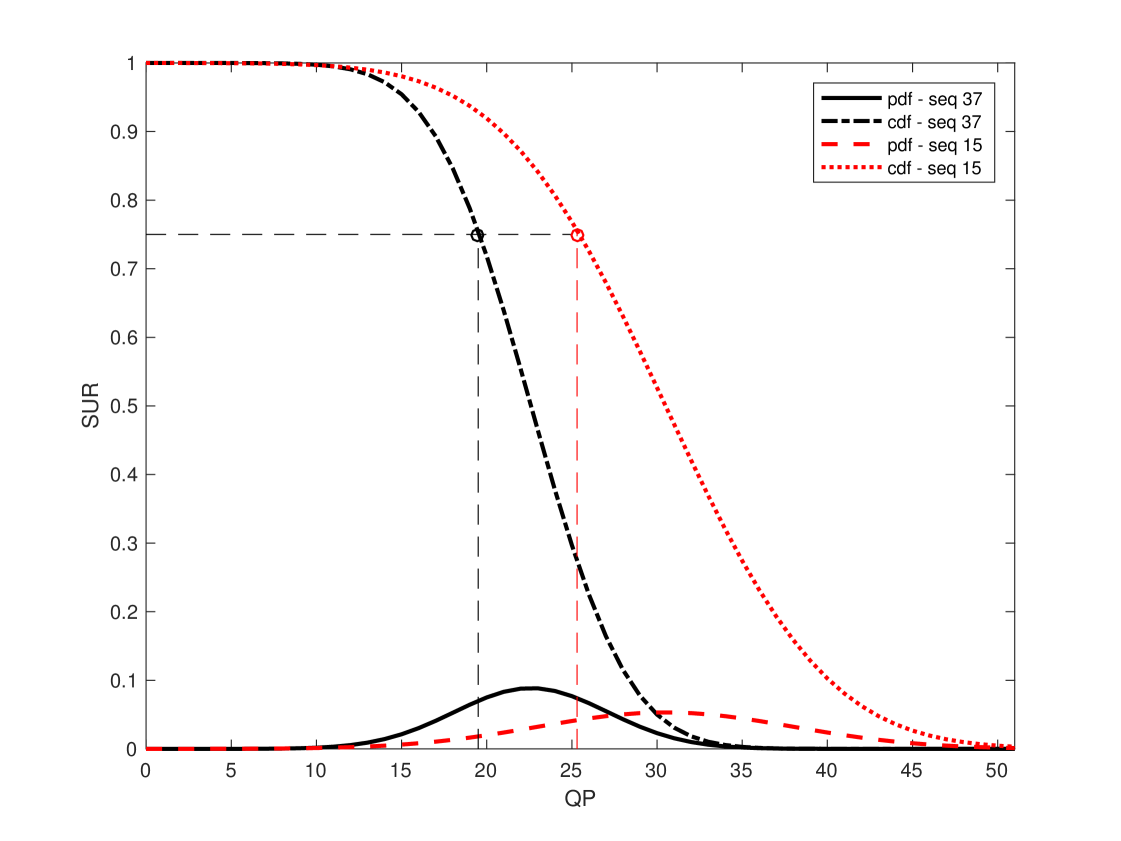
In general, we can convert a set of measured JND samples from a test sequence to its satisfied user ratio (SUR) curve through integration from the smallest to the largest JND values. For the discrete case, we can change the integration operation to the summation operation. For example, to satisfy % viewers with respect to the first JND, we can divide all viewers into two subsets - the first % and the remaining % - according to ordered JND values. Then, we can set the boundary QPp value between the two subsets as the target QP value in video coding. For the first subset of viewers, their JND value is smaller than QPp so that they can see the difference between the source and coded video clips. For the second subset of viewers, their JND value is larger than QPp so that they cannot see the difference between the source and coded video clips. We call the latter group the satisfied user group.
When we model the JND distribution as a normal distribution, the SUR curve becomes the Q-function. Two examples are given in Fig. 9, where the first JND points of sequence #15 and #37 are plotted based on their approximating normal distributions, where the mean and SD values are derived from the subjective test data. Their corresponding Q-functions are also plotted. The Q-function is the same as the SUR curve. For example, the top quartile of the Q-function gives the QP value to encode the video content whose quality will satisfy 75% of viewers in the sense that they cannot see the difference between the coded video and the source video. In other words, it is perceptually lossless compression for these viewers.
 \phantomcaption
We show four representative thumbnail images from the two examples in Fig. 10. The top and bottom rows are encoded results of sequence #15 and sequence #37, respectively. The first column has the best quality with QP=0. Columns 2-4 are encoded with the QP values of the first quartiles of the first, the second, and the third JND points. For a great majority of viewers (say, 75%), the video clip of the first JND point is perceptually lossless to the reference one as shown in the first column. The video clip at the second JND point begins to exhibit noticeable artifacts. The quality of the video clip at the third JND point is significantly worse.


The VideoSet and the SUR quality metric have the following four important implications.
-
1.
It is well known that the comparison of PSNR values of coded video of different contents does not make much sense. In contrast, we can compare the SUR value of coded video of different contents. In other words, the SUR value offers a universal quality metric.
-
2.
We are not able to tell whether a certain PSNR value is sufficient for some video contents. It is determined by an empirical rule. In contrast, we can determine the proper QP value to satisfy a certain percentage of targeted viewers. It provides a practical and theoretically solid foundation in selecting the operating QP for rate control.
-
3.
To the best of our knowledge, the VideoSet is the largest scale subject test ever conducted to measure the response of the human visual system (HVS) to coded video. It goes beyond the PSNR quality metric and opens a new door for video coding research and standardization, i.e. data-driven perceptual coding.
-
4.
Based on the SUR curve, we can find out the reason for the existence of the first JND point. Then, we can try to mask the noticeable artifacts with novel methods so as to shift the first JND point to a larger QP value. It could be easier to fool human eyes than to improve the PSNR value.
7 Conclusion and Future Work
The construction of a large-scale compressed video quality dataset based on the JND measurement, called the VideoSet, was described in detail in this paper. The subjective test procedure, detection and removal of outlying measured data, and the properties of collected JND data were detailed. The significance and implications of the VideoSet to future video coding research and standardization efforts were presented. It points out a clear path to data-driven perceptual coding.
One of the follow-up tasks is to determine the relationship between the JND point location and the video content. We need to predict the mean and the variance of the first, second and third JND points based on the calibrated dataset; namely, the VideoSet. The application of the machine learning techniques to the VideoSet for accurate and efficient JND prediction over a short time interval is challenging but an essential step to make data-driven perceptual coding practical for real world applications. Another follow-up task is to find out the artifacts caused by today’s coding technology, to which humans are sensitive. Once we know the reason, it is possible to mask the artifacts with some novel methods so that the first JND point can be shifted to a larger QP value. The perceptual coder can achieve an even higher coding gain if we take this into account in the next generation video coding standard.
Acknowledgments
This research was funded by Netflix, Huawei, Samsung and MediaTek. The subjective tests were conducted in the City University of Hong Kong and five universities in the Shenzhen City of China. They were Shenzhen University, Chinese University of Hong Kong (SZ), Tsinghua University, Peking University and Chinese Academy of Sciences. Computation for the work was supported in part by the University of Southern California’s Center for High-Performance Computing (hpc.usc.edu). The authors would like to give thanks to these companies and universities for their strong support.
References
- [1] Lin, J.Y., Jin, L., Hu, S., Katsavounidis, I., Li, Z., Aaron, A., Kuo, C.C.J.: Experimental design and analysis of JND test on coded image/video. In: SPIE Optical Engineering+ Applications, International Society for Optics and Photonics (2015) 95990Z–95990Z
- [2] Jin, L., Lin, J.Y., Hu, S., Wang, H., Wang, P., Katasvounidis, I., Aaron, A., Kuo, C.C.J.: Statistical study on perceived JPEG image quality via MCL-JCI dataset construction and analysis. In: IS&T/SPIE Electronic Imaging, International Society for Optics and Photonics (2016)
- [3] Wang, H., Gan, W., Hu, S., Lin, J.Y., Jin, L., Song, L., Wang, P., Katsavounidis, I., Aaron, A., Kuo, C.C.J.: MCL-JCV: A JND-based H.264/AVC video quality assessment dataset. In: 2016 IEEE International Conference on Image Processing (ICIP). (2016) 1509–1513
- [4] Haiqiang, W., Ioannis, K., Xin, Z., Jiwu, H., Man-On, P., Xin, J., Ronggang, W., Xu, W., Yun, Z., Jeonghoon, P., Jiantong, Z., Shawmin, L., Sam, K., Kuo, C.C.J.: Videoset: A large-scale compressed video quality dataset based on JND measurement. https://ieee-dataport.org/documents/videoset (2016)
- [5] Aimar, L., Merritt, L., Petit, E., Chen, M., Clay, J., Rullgrd, M., Heine, C., Izvorski, A.: X264-a free h264/avc encoder. http://www.videolan.org/developers/x264.html (2005) Accessed: 04/01/07.
- [6] Pinson, M.H.: The consumer digital video library [best of the web]. http://www.cdvl.org/resources/index.php (2013)
- [7] CableLabs. (http://www.cablelabs.com/resources/4k/) Accessed: 2016-11-22.
- [8] Blender Foundation, C. (mango.blender.org) Accessed: 2016-11-22.
- [9] Ou, Y.F., Xue, Y., Wang, Y.: Q-star: a perceptual video quality model considering impact of spatial, temporal, and amplitude resolutions. IEEE Transactions on Image Processing 23 (2014) 2473–2486
- [10] Turkowski, K.: Graphics gems. Academic Press Professional, Inc., San Diego, CA, USA (1990) 147–165
- [11] Sharma, G., Bala, R.: Digital color imaging handbook. CRC press (2002)
- [12] Grubbs, F.E.: Sample criteria for testing outlying observations. The Annals of Mathematical Statistics (1950) 27–58
- [13] Jarque, C.M., Bera, A.K.: A test for normality of observations and regression residuals. International Statistical Review/Revue Internationale de Statistique (1987) 163–172
- [14] Lin, W., Jay Kuo, C.C.: Perceptual visual quality metrics: A survey. Journal of Visual Communication and Image Representation 22 (2011) 297–312