Vietoris-Rips Complexes of Split-Decomposable Spaces
Abstract
Split-metric decompositions are an important tool in the theory of phylogenetics, particularly because of the link between the tight span and the class of totally decomposable spaces, a generalization of metric trees whose decomposition does not have a “prime” component. We use this connection to study the Vietoris-Rips complexes of totally decomposable spaces. In particular, we characterize the homotopy type of the Vietoris-Rips complex of circular decomposable spaces whose metric is monotone. We extend this result to compute the homology of certain non-monotone circular decomposable spaces. We also use the block decomposition of the tight span of a totally decomposable metric to induce a decomposition of the VR complex of a totally decomposable metric.
1 Introduction
Split-metric decompositions are an important tool in the theory of phylogenetics, particularly because of the link between the tight span and the class of totally decomposable spaces, a generalization of metric trees whose decomposition does not have a “prime” component. The connection with tight spans has been studied at least since the introduction of split-metric decompositions by Bandelt and Dress in [BD92], and culminated with the characterization of the polytopal structure of the tight span of a totally decomposable metric by Huber, Koolen, and Moulton in [HKM19]. A special type of totally decomposable spaces are the circular decomposable spaces introduced in [BD92]. Intuitively, a space is circular decomposable if there is a bijection from the vertices of a regular -gon inscribed in the circle in such a way that the points of can be “separated” in the same way that is separated by a line. See Definition 2.10 for a precise description.
We study the Vietoris-Rips (VR) complexes of totally decomposable spaces using two central results in Topological Data Analysis. One is the characterization of the VR complexes of subsets of the circle by Adamaszek and Adams [AA17]. Given the similarity between circular decomposable spaces and subsets of the circle, we investigate how similar their VR complexes are. In Section 3, we use the results of [AA17] to characterize the homotopy type of circular decomposable spaces whose metric is also monotone in the sense of [Far97] (see Theorem 3.14). We also give conditions on the isolation indices of a circular decomposable space that guarantee the metric to be monotone (Corollary 3.13). However, not every circular decomposable metric is also monotone. In Section 4, we compute the homology of circular decomposable spaces in terms of a strict subset (Theorems 4.7 and 4.8). The results on the homotopy type of clique complexes of cyclic graphs [AA17] are instrumental in this section.
Lastly, in Section 5, we study how the block decomposition of the tight span of a totally decomposable metric affects the VR complex of . Our main result in this section is that the VR complex of decomposes as a disjoint union or wedge of the VR complexes of certain subsets , each corresponding to a block in the tight span (Theorem 5.12). We then compute the homology of as a direct sum of the homology groups of all , with a small modification for (Theorem 5.13).
Acknowledgments.
The author thanks Facundo Mémoli for introducing him to the paper [BD92] and for useful discussions and suggestions during the writing of this paper. The author also acknowledges funding from BSF Grant 2020124 received during the time he was finishing his PhD.
2 Preliminaries
In this section, we set the notation and collect the most important theorems and definitions from our sources.
2.1 Notation
Let be a metric space. The diameter of is . The (open) Vietoris-Rips complex (or VR complex for short) is the simplicial complex
We model the circle as the quotient and equip it with the geodesic distance scaled so that has circumference 1. We say that a path is clockwise if any lift is increasing – this defines the clockwise direction on .
Definition 2.1 (Cyclic order).
Given three points , we define the cyclic order by setting if the clockwise path from to contains . We use to indicate that .
Definition 2.2 (Circular sum).
Fix and consider a function . Given , we define the circular sum as
when and
when . The value of will be clear from context.
Remark 2.3.
The expression when usually represents an empty sum and its value is 0 by convention, while the notation is usually not 0. However, the degenerate cases in some results (like those in Section 3.2) could involve empty circular sums. Since we are deviating from the above convention, we never write empty circular sums, and always state degenerate cases separately if they would require an empty circular sum.
Two equivalent formulations of the circular sum are:
In fact, we think of as a summation of over the vertices of a regular -gon inscribed on the circle. Indeed, if we label the vertices clockwise from to , the sum adds the value of at all the vertices in the clockwise path between the -th and the -th vertices (inclusive). If , the clockwise path starting at the -th vertex has to go through the -th vertex before getting to the -th vertex.
2.2 Background
Split systems.
Our main object of study is the split-metric decomposition of a finite metric. Given a finite set , a split is a partition of . We denote splits by , , or where is the complement of in . Given , we denote by the element of that contains . A collection of splits is called a split system. A weighted split system is a pair where . We write the value of at as .
Weakly compatible split systems.
A split system is weakly compatible if there are no three splits and four elements such that
Any finite metric space has an associated weakly compatible split system (which could be empty) with weights induced by the metric. For any (not necessarily distinct), define
If is a split of , the isolation index of is the number
Note that and, as a consequence, . If , the split is called a -split. The set
is called the system of -splits of and it is weighted by the isolation indices . Bandelt and Dress proved that is always weakly compatible [BD92, Theorem 3]. However, not every metric space has -splits. We call such a space split-prime [BD92].
Example 2.4.
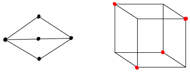
The complete bipartite graph with the shortest path metric has no -splits. It is not hard to prove (see also the introduction of Section 2 of [BD92]) that any -split must be -convex in the sense that and implies (likewise for ). It can be checked that cannot be split into two -convex sets, so it is prime. The hypercube graph with the shortest path metric is also split-prime for (see the description after Proposition 3 in [BD92]).
Split-metric decompositions.
Given a finite set and a split of , a split-metric is the pseudometric defined by
One of the main results of Bandelt and Dress is the decomposition of any finite metric as a linear combination of split-metrics and a split-prime residue.
Theorem 2.5 ([BD92, Theorem 2]).
Any metric on a finite set decomposes as
| (1) |
where is split-prime and the sum runs over all -splits . Moreover, the decomposition is unique in the following sense. Let be a weakly compatible split system on with weights for . If , then there is a bijection such that .
Equation (1) is called the split-metric decomposition of , or split decomposition for brevity.
Remark 2.6.
Definition 2.7.
Given a weighted weakly compatible split system on , we define the pseudometric
Definition 2.8 (Totally decomposable spaces).
A metric space is called totally decomposable if in Equation (1). Equivalently, where and is the isolation index of .
Circular collections of splits.
Suppose is a set with points. Then a weakly compatible split system on can have at most splits. The reason is that the vector space of symmetric functions with diagonal has dimension and the uniqueness in Theorem 2.5 implies that the set of split-metrics is linearly independent [BD92, Corollary 4].
There are examples of split systems that achieve this bound. Let be the vertices of a regular -gon. Any line that passes through two distinct edges and separates into the sets and . Since there are edges, this construction gives a split system with different splits, and it can be verified that is weakly compatible. It turns out that, up to a bijection of the underlying sets, this is the only example.
Theorem 2.9 ([BD92, Theorem 5]).
The following conditions are equivalent for a weakly compatible split system on a set with :
-
1.
;
-
2.
There exists a bijection such that ;
-
3.
The set is a basis of the vector space of all symmetric functions with 0 diagonal.
Note that such an inherits the cyclic order from . Explicitly, if we define , then if and only if .
We later study not only but its subsets as well.
Definition 2.10.
Let be a split system on a set . If there exists a bijection such that , we say that is a circular split system. Likewise, a finite metric space is circular decomposable if is circular. If in addition , we say that is a full circular system. We define full circular decomposable metrics analogously.
Clique complexes of cyclic graphs.
The main tool used in [AA17] to compute the homotopy type of were the directed cyclic graphs. We give an undirected definition.
Definition 2.11.
Let be a graph with vertex set such that . We say that is cyclic if has a cyclic order and there exists a function such that the following two conditions hold:
-
•
For any , if is an edge of , then is an edge of .
-
•
For any , if is an edge of , then is an edge of .
We also make the following definition for convenience.
Definition 2.12.
A clique complex is called cyclic if its 1-skeleton is cyclic. Similarly, we define when is cyclic.
Note that we can give an orientation to our cyclic graphs by orienting an edge from to if or . Thanks to this, the results of [AA17] also hold for undirected cyclic graphs.
Theorem 2.13 ([AA17, Theorem 4.4]).
If is a cyclic graph, then
We are mainly interested in studying metric spaces whose VR complexes are cyclic.
Definition 2.14.
A metric space with is monotone111We adopted the term “monotone” from [Far97]. if it has a cyclic order and there exists a function such that the following two conditions hold:
-
•
For any , we have .
-
•
For any , .
It is not hard to see that the VR complexes of a monotone metric space are cyclic for any .
Buneman complex.
There is a polytopal complex associated to any weakly compatible split system on with weights . Let
Given , let . Define
Note that is polytope isomorphic to a hypercube of dimension . The Buneman complex of is defined by
Both and are equipped with the metric:
The space admits an isometric embedding of via the map where
Tight span.
Let be a metric space. The tight span of is the set such that for all :
-
1.
for all ;
-
2.
for all .
These properties imply, in particular, that for all and .The tight span is equipped with the metric
and there exists an isometric embedding defined by
Tight spans are examples of injective metric spaces. A metric space is injective if for every 1-Lipschitz map and for every isometric embedding , there exists a 1-Lipschitz extension that makes the following diagram commute:
In particular, is the smallest injective space that contains , i.e. for any injective such that . Furthermore, injective spaces have nice topological and geometric structures.
Proposition 2.15.
Any injective metric space is contractible and geodesic.
See the comment after Proposition 2.1 of [LMO22].
Tight spans are an important tool in topological data analysis thanks to Theorem 2.16 below. We need one more definition before stating this result. Given a metric space , and , the metric thickening of in is the set
If there is an isometric embedding , we will write instead of .
Theorem 2.16 ([LMO22, Proposition 2.3]).
Let be a metric space, and let be an injective space such that . Then the Vietoris-Rips complex and the metric thickening are homotopy equivalent for every .
Tight spans of totally decomposable metrics.
The tight span of totally decomposable metrics has been studied by several authors throughout the years [BD92, DH01, HKM06, HKM19]. We use the notation and results of [HKM19], one of the most recent papers. Given a weighted split system on , define the map
where is the metric on . The first salient property of is that it sends each element to . In other words, is “constant” on the embedded copy of inside the Buneman complex and the tight span. The map has much stronger properties when is weakly compatible.
Theorem 2.17.
Let be a weighted split system on . The map is 1-Lipschitz. Furthermore, if and only if is weakly compatible.
See the introduction to Section 4 of [HKM06] to see why and why is 1-Lipschitz. The equivalence between and weak compatibility is the main result of [DHM98].
Remark 2.18.
The map also induces a strong relationship between the polytopal structures of the Buneman complex and the tight span. We need more definitions to state this result.
Let be a connected polytopal complex. A vertex is a cut-vertex if is disconnected. A maximal subcomplex that does not have cut-vertices is called a block. The set of blocks of is denoted as . The block structure of the Buneman complex can be determined from the properties of in a straightforward way.
Definition 2.19.
Let be a split system on . Two splits are called compatible if the following equivalent conditions hold:
-
•
There exist , with ;
-
•
There exist , with ;
-
•
There exist , with or .
If neither condition holds, we say that and are incompatible. We define the incompatibility graph to be the graph with vertex set and edge set consisting of all pairs where and are distinct incompatible splits.
Theorem 2.20.
Let be a weighted split system on . There is a bijective correspondence between the connected components of the incompatibility graph and the blocks of . Moreover, for every , the block corresponding to is isomorphic as a polytopal complex to .
We denote the block of corresponding to as .
We need one more definition before stating the link between the polytopal structures of and . A split system is called octahedral if and there exists a partition such that for (indices are taken modulo 6) and .
Theorem 2.21.
Let be a weighted weakly compatible split system on . Then induces a bijection between and such that:
-
•
If is not octahedral, then the block is isomorphic to the block as polytopal complexes.
-
•
If is octahedral, then is a block isomorphic to a rhombic dodecahedron.
3 Properties of circular decomposable metrics
According to Theorem 2.9, a split system on with maximal cardinality is necessarily circular. In this section, we investigate the properties of a circular decomposable metric space .
We fix throughout this section. We assume that and that the bijection from Theorem 2.9 satisfies . If is a full circular system, the splits have the form where and . Note that there are splits of the form and that they are all distinct. Then if , we have
| (2) |
by Theorem 2.5. If is circular but not full, then (see Definition 2.10). In that case, we set for any split and Equation (2) still holds. We write for any . Recall that inherits the cyclic order from (see Definition 2.1) so that if the clockwise path from to contains .
3.1 An expression for in terms of
Our objective in this section is to find an expression for that does not contain any terms. For that, it will be convenient to extend the definition of and to any . In fact, the current expression for when is equivalent to, so we extend this definition to any . Notice that:
-
•
If , for ;
-
•
If , unless ;
-
•
If and or , then .
Hence, we define:
-
•
For and , and where indices are taken modulo (unless and or );
-
•
If , we set and leave undefined.
The reason to leave undefined if (which includes the case of and ) is because forces . A pair is only a valid split if both and are non-empty. However, defining the coefficients as 0 will be convenient for later calculations.
Remark 3.1.
We summarize the above discussion for future reference. For any , the set is defined as , and the isolation indices satisfy the relations
-
•
, and
-
•
.
If , we define the split , which satisfies the relation .
Lemma 3.2.
Let . Then (indices are treated modulo ). The analogous equation holds if we replace with .
Proof.
Lemma 3.3.
For any with , .
3.2 Monotone circular decomposable metrics
Given that circular split systems have such a close relationship with finite subsets of , we want to explore how similar their VR complexes are. A crucial feature of subsets of is that their VR complexes are cyclic. However, this is not the case for every circular decomposable metric.
Example 3.4.
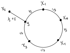
Consider the wedge of and an interval as shown in Figure 2. Let and . has a circular split system and all its VR complexes are cyclic because . Since for , it follows that . Hence, also has a circular split system and it inherits the cycic order from so that . However, , so is not cyclic for . Intuitively, the edge appears in before either or even though is “between” and .
Given that not every circular decomposable metric space has cyclic VR complexes, we look for conditions on the isolation indices that force the VR complexes to be cyclic. We begin with the following Lemma.
Lemma 3.5.
If , we have
-
•
if and only if .
-
•
if and only if .
Proof.
In order for the VR complex of to be cyclic, we need to be an edge of whenever is. Similarly, must be an edge whenever is, and so on. In the other direction, must be an edge whenever is. Rephrasing these conditions in terms of the metric shows that, at a minimum, we need
| (3) |
for some . We give a name to this condition.
Definition 3.6.
Let be a metric space with a cyclic order . We say that is unimodal at if there exists such that:
-
•
for all , and
-
•
for all .
We denote the minimal such as .
Unimodality by itself is not enough to guarantee monotonicity of , but it is pretty close.
Lemma 3.7.
Let be a finite metric space with a cyclic order . If is unimodal at every point and if and only if , then is monotone.
Proof.
Suppose . By hypothesis, implies . Hence, . By unimodality at , . Similarly, implies , so unimodality at implies . The second condition in Definition 2.14 follows by exchanging for in the argument above. ∎
For the remainder of the section, we find conditions on the isolation indices so that the circular decomposable metric is monotone. It turns out that we can prove many more inequalities using the properties of circular decomposable metrics.
Lemma 3.8.
Let be a circular decomposable metric space. Then for any ,
As a consequence, if and , then .
The proof of Lemma 3.8 uses the fact that the sum is at its smallest when and increases as cycles through . Likewise, the sum achieves its maximum when and steadily decreases in the same range. It turns out that the point when becomes larger than determines whether is monotone or not, and we give this point a name.
Definition 3.9.
Let be a circular decomposable metric and fix . We define to be the first element of the sequence such that:
-
•
when ; and
-
•
when .
Let’s prove that determines .
Lemma 3.10.
Let be a circular decomposable metric. Suppose there exists a value such that if and only if . Then is unimodal at and .
Proof.
Heuristically, if all isolation indices have roughly the same value, the distances and should be similar. In consequence, we could expect the following property to hold:
| () |
Throughout the following lemmas, we show that a circular decomposable metric that satisfies this assumption must be monotone. We start by proving the existence of an that satisfies the conditions of Lemma 3.10. This will give a way to find using .
Lemma 3.11.
Let be a circular decomposable metric that satisfies Property ( ‣ 3.2). Let be the last in the sequence such that . Then satisfies if and only if .
Proof.
By definition of , holds for any . Thus, we only need to verify the lemma for . By Property ( ‣ 3.2) and the definition of , . Hence, . ∎
Lemma 3.12.
Let be a circular decomposable metric that satisfies Property ( ‣ 3.2). Then if and only if .
Proof.
We first show that implies . Let be an element of the sequence . By Lemmas 3.10 and 3.11, is the last value that satisfies . Our objective is to determine the range of values of in which can appear.
First, we show that occurs after . If , Lemma 3.11 implies that . Property ( ‣ 3.2) gives , which combines with the previous inequality to give . In particular, satisfies that condition, so occurs at the same time or after .
Now we show that cannot occur after . If , the characterization of says that . By Property ( ‣ 3.2), . Hence, . Thus, does not hold, so cannot occur after . This finishes the proof that , and the proof of is analogous.
∎
Corollary 3.13.
Any circular decomposable metric that satisfies Property ( ‣ 3.2) is monotone.
Proof.
With the previous corollary, we can write a formula for the homotopy type of the VR complex of any circular decomposable metric that satisfies Property ( ‣ 3.2).
Theorem 3.14.
Let be a circular decomposable metric that satisfies Property ( ‣ 3.2) and fix . Let be the 1-skeleton of . Then
4 Non-monotone circular decomposable metrics
In this section, we describe how to compute the homology groups of circular decomposable metrics that are not monotone. However, circular decomposable metrics are not too far from being monotone, so we can use the properties of monotone metrics and cyclic graphs to compute the homology of more general circular decomposable metrics. Concretely, our strategy to compute will be to split into the cyclic piece and the non-cyclic piece, compute the homology of the cyclic piece with 2.13, and use the Mayer-Vietoris sequence to find the homology of .
4.1 Cyclic component of for a circular decomposable non-monotone .
Fix and suppose is a circular decomposable metric. For ease of notation, we denote with and its 1-skeleton with . We use the following function to test if is monotone.
Definition 4.1.
Let be a circular decomposable metric and fix . Given , let be the last in the sequence such that for all .
Notice that for any , both and are smaller than , so holds. However, we don’t know if the same implication holds when . This implication holds if is monotone and, in that case, we can use the results from the previous section to find . If is not monotone, there exists and such that . Intuitively, is not cyclic because the edge appeared at a lower than it was supposed to. These are the edges we want to remove, so we set
Definition 4.2.
Let and suppose is a circular decomposable metric. We form a graph by removing the edges in from and define . We call the cyclic component of .
By definition, is a cyclic complex because we removed the edges that made non-cyclic. Plus, if was cyclic to begin with, then . On the other hand, let be the vertex set of , the closed star of in . Notice that the subcomplex of induced on equals and .
Intuitively, we have separated into its cyclic part and the subcomplex induced by edges that prevent from being cyclic. We want to use these complexes and the Mayer-Vietoris sequence to compute the homology of , and there are a couple of facts to verify. First, let .
Lemma 4.3.
is a cyclic clique complex.
Proof.
Firstly, note that inherits the cyclic order from so that . Also, is a clique complex because both and are. To verify that is cyclic, define by setting to be the last from the sequence such that .
Let such that . To show that is cyclic, we have to prove that implies . If , the fact that is cyclic and means that . This also implies that because is the induced subcomplex of on . Hence, . The second condition in Definition 2.11 follows analogously.
∎
Now we make sure that we didn’t lose any simplices when splitting into and .
Lemma 4.4.
.
Proof.
Let be a simplex of . If does not contain an edge from , then by definition of . If does contain an edge from , then . ∎
Lastly, we record the following for future use.
Proposition 4.5.
Let , , and be the natural inclusions. The homology groups of , , , and satisfy the following Mayer-Vietoris sequence:
| (4) |
4.2 Recursive computation of .
There is an obstacle to using Proposition 4.5. If , equals because we defined as an induced subcomplex. We would also have , which means that the Mayer-Vietoris sequence would give the trivial statements and . Hence, we assume in this section.
First we focus on finding when is in the non-critical regime, i.e. for some . We begin with a technical property.
Lemma 4.6.
Let , , , be group homomorphisms and suppose
is exact. If is an injection/surjection/isomorphism, then so is .
Proof.
Suppose is injective. If , then . By exactness, there exists such that and . Since is injective, , so .
Suppose is surjective. Given , there exist and such that by exactness. Also, there exists such that by assumption. Exactness implies that . Thus, .
∎
Theorem 4.7.
Suppose .
-
1.
If is injective and is torsion-free, then
-
2.
If , then
Proof.
Recall Proposition 4.5:
By Theorem 2.13, equals if and 0 otherwise, so for . The remaining part of the sequence is as follows:
| (5) | ||||
If is injective, then so is and the bottom row becomes a short exact sequence. This forces , so .
Finding requires two cases depending on whether is trivial or not. If , the fact that the bottom row of (5) is a short exact sequence yields . If , we must have by Theorem 2.13. The inclusion of cyclic complexes is induced by the inclusion of their 1-skeleta which, in turn, is a cyclic homomorphism of cyclic graphs by [AA17, Lemma 3.6]. Then, by [AA17, Proposition 4.9], . Hence, is an isomorphism, so Lemma 4.6 gives that is an isomorphism. Moreover, since is torsion-free by hypothesis, the short exact sequence
splits. Thus,
In our second claim we have . In particular, is surjective. The reasoning in the paragraph above shows that is either 0 or isomorphic to , and in either case, is surjective. Hence, is surjective, so by exactness of (5). This observation also implies that (5) reduces to
Lastly, the fact that or implies that this sequence becomes a split short exact sequence upon replacing the terms with . This finishes the proof. ∎
Now assume for some . Unlike the non-critical regime, usually has more than one generator.
Theorem 4.8.
Suppose for some . Let and be the kernel and coimage, respectively, of the map . If both and are free, then
Proof.
5 Wedge decomposition of .
In the last section, we use the block decomposition of the Buneman complex and the tight span to show that decomposes as a wedge sum of smaller VR complexes. During this section, we assume that is a totally decomposable space that is not necessarily circular decomposable.
Let’s find the split decomposition of a subset of that determines a block.
Definition 5.1.
Let be a weighted weakly compatible split system on . Let and define . We define a weighted split system on as follows. For each , define
Set , and define by where the sum runs over all that extend . We denote by .
Lemma 5.2.
If for some , . As a consequence, is weakly compatible.
Proof.
Let . Since is a block of , the connected component that contains is different from . In other words, , so by [HKM19, Theorem 7], for any and . Then
Let . If , then and . The same holds if . On the other hand, if and , then and while and . In other words,
The same holds if and , so
The last equation holds because a split can only extend . By Theorem 2.5, . The lemma follows because restricts to in . ∎
Recall that the map between the Buneman complex and the Tight span is not an isometry in general. However, it does preserve the distance from an element in the Buneman complex to every point in the embedding of .
Proposition 5.3.
Let be a weighted weakly compatible split system on . For any and ,
As a consequence, the map sends onto .
Proof.
Let . Observe that
Since , the reverse triangle inequality yields . This upper bound is actually realized when we set , so . Lastly, observe that maps onto because
∎
Now we use the block structure of the Buneman complex to induce a decomposition of the VR complex of in terms of the VR complex of each for each .
Definition 5.4.
Let be a weighted weakly compatible split system on , and let be the set of cut-vertices of . Let be the graph that has vertex set . We draw an edge between any and every block such that .
We think of as the skeleton of . We make each block in into a vertex and join two intersecting blocks through a path where is the cut-vertex in the intersection of and . Moreover, has a simple structure because the tight span is contractible.
Lemma 5.5.
The graph is a tree.
Proof.
Recall that the tight span of any metric space is contractible (Proposition 2.15). In particular, each block is contractible and deformation retracts onto a space homeomorphic to the star of as a vertex of through a homotopy that fixes the cut-vertices in . Thus, deformation retracts onto through a homotopy relative to . must then be a contractible graph, hence a tree. ∎
On the other hand, the fact that is a tree has implications for the tight span.
Lemma 5.6.
For every , the block is a hyperconvex space, hence injective.
Proof.
Let and such that . To prove that is hyperconvex, we need to find such that for all . We know that is injective, so there exists a point that satisfies . If , we are done. If not, we claim there exists a unique cut-vertex such that and are in different connected components of . First, recall that is a block of by Theorem 2.21, so there exists a cut-vertex that separates from . If there were two such that both and separated from , then there would be a sequence of blocks and cut-vertices of such that
This induces a non-trivial cycle in , which cannot exist by Lemma 5.5. This verifies the uniqueness of . Since is geodesic, there exist geodesics from to of length less than . Since separates from , these geodesics must contain . Hence, and . Hence, is hyperconvex. ∎
Notice that the block structure of induces a decomposition of . By Theorem 2.16, is homotopy equivalent to , and this decomposes into the union of the intersection of with each block of . However, thanks to Lemma 5.6, we will prove that this intersection is the VR complex of a subset of . That subset is given by the following definition.
Definition 5.7.
Let . For each edge , consider all the points such that and are in different connected components of . Among those, choose to be any point that minimizes and define
We verify that the above definition does not depend on the choices of .
Lemma 5.8.
The isometry type of is independent of the choice of .
Proof.
Our strategy will be to show that for any choice of and for , the distances between and every point in depends only on and and . Thus, given , let be any point such that is in the connected component of that does not intersect . By Theorem 2.21, is a cut-vertex of . This, together with the fact that the tight span is geodesic (Proposition 2.15), implies that
| (6) |
for any . In particular, this holds for for any . Hence, only depends on . Since minimizes , the distance does not depend on the choice of . If is another cut-vertex in , we set in the above equation and get
Moreover, any geodesic from to goes through by definition of . Swapping the roles of and implies that a geodesic from to passes through both and , so
which, again, does not depend on the choice of and . ∎
Lemma 5.9.
Let . Let be the space formed by attaching an edge of length to at for every cut-vertex . Then is injective and .
Proof.
By Lemma 5.6, the block is an injective space. Let be a line segment of length for every cut-vertex . A line segment with the usual metric is hyperconvex hence injective, and the wedge of two injective spaces is injective by [LMO22, Lemma 6.2]. Hence, is injective. Now consider the map that sends each to and each to the boundary point of that is different from . By equation (6), is an isometric embedding. ∎
Below we realize the VR complex of as a subset of a block of .
Lemma 5.10.
If ,
Proof.
Let be the connected components of . If , equation (6) implies that is a ball centered at of radius . If , then . Hence, equals union with the balls centered at of radius for those for which .
On the other hand, let be the injective space from Lemma 5.9. Let be the edge attached at for . A homotopy equivalence that contracts the edges of of length less than to their gluing points in induces a homotopy equivalence . We can then apply a homotopy equivalence to contract every edge to whenever . Thus, by Theorem 2.16,
∎
Definition 5.11.
Given and a choice of for each , we define as follows. For each block ,
-
•
Replace the vertex with one vertex for each connected component of .
-
•
An edge of the form is replaced with the edge if and (if any).
Note that, similarly to Lemma 5.8, does not depend on the specific choice of .
Now, think of as an indexing category where an edge with becomes an arrow . Define a functor by
sends each arrow to the inclusion map .
This functor encodes the block decomposition of .
Theorem 5.12.
For any ,
Proof.
Given , let . Notice that any two , intersect in a common cut-vertex if and only if has edges . Let denote the identification of the point and the point whenever are edges of . Then
Then by Theorem 2.16,
∎
The work of this section pays off below. We prove that the homology of the VR complex of decomposes in terms of the homology of .
Theorem 5.13.
Let be a totally decomposable metric with split system . For any ,
For , the equation holds after identifying the class of with the class of any for which .
Proof.
Let be the connected components of and let be their corresponding blocks in . Let and . Lastly, let . We claim that
| (7) |
The claim is clear for . For , we have the Mayer-Vietoris sequence
Notice that is either empty or a cut-vertex , so is a set of isolated points. Hence, (7) holds for . In order for the claim to hold for , we need the boundary map to be 0. This happens if and only if the map
is injective. In other words, we need to show that if any pair of non-empty intersections and has , then and belong to different connected components of or . Indeed, this must happen by Lemma 5.5 because if both and belonged to the same connected components of and , then would have a cycle. Hence, (7) holds for all . The theorem for now follows from Lemma 5.10.
Lastly, let . Every point belongs to the for which . However, could also belong to if for some , . This introduces duplicate connected components in . We get the correct after identifying these classes.
∎
References
- [AA17] Michał Adamaszek and Henry Adams. The Vietoris-Rips complexes of a circle. Pacific Journal of Mathematics, 290(1):1–40, 2017.
- [BD92] Hans-Jürgen Bandelt and Andreas Dress. A canonical decomposition theory for metrics on a finite set. Advances in Mathematics, 92(1):47–105, 1992.
- [DH01] Andreas Dress and Katharina T. Huber. Totally split-decomposable metrics of combinatorial dimension two. Annals of Combinatorics, 5(1):99–112, Jun 2001.
- [DHM98] Andreas Dress, Katharina T. Huber, and Vincent Moulton. A comparison between two distinct continuous models in projective cluster theory: The median and the tight-span construction. Annals of Combinatorics, 2(4):299–311, Dec 1998.
- [Far97] Martin Farach. Recognizing circular decomposable metrics. Journal of Computational Biology, 4(2):157–162, 1997. PMID: 9228614.
- [HKM06] Katharina T. Huber, Jack H. Koolen, and Vincent Moulton. On the structure of the tight-span of a totally split-decomposable metric. European Journal of Combinatorics, 27(3):461–479, 2006.
- [HKM19] Katharina T. Huber, Jack H. Koolen, and Vincent Moulton. The polytopal structure of the tight-span of a totally split-decomposable metric. Discrete Mathematics, 342(3):868–878, 2019.
- [LMO22] Sunhyuk Lim, Facundo Memoli, and Osman Berat Okutan. Vietoris-Rips persistent homology, injective metric spaces, and the filling radius. Algebraic and Geometric Topology, 2022.