Viewport Prediction for Volumetric Video Streaming by Exploring Video Saliency and Trajectory Information
Abstract
Volumetric video, also known as hologram video, is a novel medium that portrays 3D content in extended reality. It is expected to be the next-gen video technology and a prevalent use case for 5G and beyond wireless communication. Considering that each user typically only watches a section of the volumetric video, known as the viewport, it is essential to have precise viewport prediction for optimal streaming performance. However, research on this topic is still in its infancy. To this end, this paper proposes a novel approach, Saliency and Trajectory Viewport Prediction (STVP), to improve the precision of viewport prediction in volumetric video streaming by extensively exploiting the video saliency and viewport trajectory information. In particular, we introduce a novel sampling method, Uniform Random Sampling (URS), to efficiently preserve video features while reducing computational complexity. Then we propose a saliency detection technique that combines spatial and temporal information for detecting visually static and dynamic geometric, and luminance salient regions. Finally, we fuse saliency and trajectory information to achieve more accurate viewport prediction. Extensive experimental results validate the superiority of our method over existing state-of-the-art schemes. The dataset and source code will be publicly accessible after acceptance. To the best of our knowledge, this is the first comprehensive study of viewport prediction in volumetric video streaming.
Index Terms:
viewport prediction, volumetric video, trajectory prediction, saliency detection, samplingI Introduction
Volumetric video, also known as holographic video, allows users to fully immerse themselves in a 3D scene and move freely in any direction, providing 6 degrees of freedom (6DoF) experience [1, 2]. Typically, users watch only a section of a video, referred to as a “viewport”111Viewport, also referred to as the field of view (FoV), is the portion of a video that a user actually watches. In this paper, we use “viewport” and “FoV” interchangeably., at a time and are allowed to switch between viewports freely at will. This versatility makes volumetric video to be expected to become the next-generation video technology for entertainment, education, and manufacturing applications, among others [3, 4].
Point cloud video is a prevalent kind of volumetric video, presenting various challenges due to the high bandwidth and low latency requirements for transmission. Many works adopt tiling and adaptive streaming technologies to address these limitations [5] by allowing the server to transmit only the tiles within the user’s viewport [6]. However, an inaccurate estimate of the viewport may lead to a deterioration in the user’s viewing experience. Hence, accurate viewport prediction is critical for optimal point cloud video transmission, as illustrated in Fig. 1.
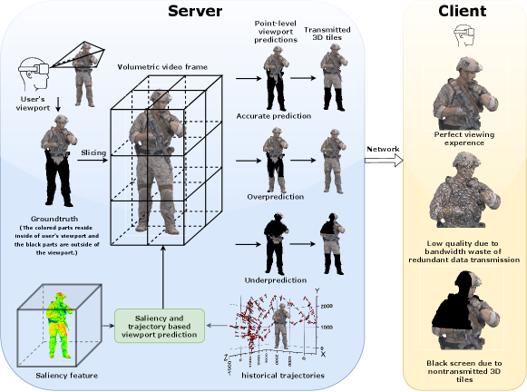
When watching point cloud videos, users are often attracted to visually salient content, such as vibrant hues, noticeable geometric shapes, and motion. Relatedly, the user trajectory consists of head position and orientation and exhibits temporal coherence, which can be predicted with deep learning techniques[7]. Therefore, the saliency features of a point cloud video and the user’s trajectory can be used to accurately predict the user’s viewport. Depending on the information used for prediction, there are usually three alternatives to perform viewport prediction for point cloud video.
(1) Trajectory based viewport prediction. The user’s trajectory exhibits temporal coherence, allowing us to infer the state at the next moment based on the preceding historical trajectory.
(2) Saliency based viewport prediction. Visual saliency detection is designed to identify areas that users are likely to view [8]. Therefore, visual saliency detection serves as a method for predicting user viewports. The investigation of saliency prediction in 360-degree videos has seen considerable advancemen[9, 10, 11, 12]. However, to the best of our knowledge, there is still a gap in dynamic saliency detection for 6DoF volumetric video systems.
(3) Saliency and Trajectory based hybrid prediction. To further improve the prediction accuracy, multi-modal methods that combine video saliency and trajectory are also proposed [13, 14, 15].
Despite significant efforts directed toward predicting user viewports, viewport prediction in volumetric video systems is still in its early stages. The technical challenges are as follows:
Lack of efficient techniques in temporal feature extraction for large-scale point cloud videos: The dense nature of point cloud videos imposes considerable computational demands. Conversely, for the temporal feature extraction of large-scale point cloud videos, it is advantageous to calculate the motion intensity of moving parts instead of processing all points to mitigate the computational costs.
Deficiency in sampling method preserving temporal information for large-scale point cloud videos: During the training of a network for saliency detection in point cloud videos, it’s crucial to identify a sampling method tailored to point cloud videos. The goal is to reduce the number of points while preserving both temporal and spatial information, all while maintaining lower time complexity. Currently, existing heuristic sampling methods [16, 17, 18, 19], primarily designed for static point cloud images, may not be directly applicable to point cloud videos. Meanwhile, some heuristic sampling methods may sacrifice time information, while others exhibit high computational complexity (explained in Section II). Hence, it is important to design a suitable sampling method to enhance the point cloud video sampling.
Inadequacy in encoding techniques for capturing local visual saliency discrepancies: Additionally, in a point cloud video frame, regions with significant geometric variations and brightness changes are particularly captivating to viewers. The current spatial aggregator [20, 21, 22] focuses solely on encoding local point coordinates to extract geometric features, neglecting the importance of local luminance information. This limitation hinders an accurate representation of spatial saliency features within a single frame of a point cloud video. Therefore, it is crucial to design a spatial encoder that effectively integrates both geometric and luminance information from a single video frame.
This paper proposes a high-precision viewpoint prediction network based on some neural networks, like LSTM to address the challenges. Initially, a low-complexity 3D tile-based uniform random sampling (URS) unit is introduced, which combines spatial uniform partitioning, random sampling, and the K-nearest neighbor (KNN) method to preserve as much temporal and spatial information of the point cloud video as possible during the sampling process. By improving the efficiency of our sampling process, the corresponding sampling results for adjacent frames ascertain the feasibility of the saliency detection module.
| Reference | Video Type | Degree of Freedom | Using head trajectory | Using video saliency | Network |
| [23] | 360∘ video | 3DoF | ✔ | ✖ | WLR |
| [24] | 360∘ video | 3DoF | ✔ | ✖ | LR&KNN |
| [25] | 360∘ video | 3DoF | ✔ | ✔ | LSTM |
| [13] | 360∘ video | 3DoF | ✔ | ✔ | PanoSalNet |
| [14] | 360∘ video | 3DoF | ✔ | ✔ | Graph Learning |
| [7] | VR | 6DoF | ✔ | ✖ | LSTM&MLP |
| Our | Point cloud video | 6DoF | ✔ | ✔ | LSTM&Saliency Detection |
This paper also proposes a local feature comparison method for extracting temporal saliency features. This technique is achieved through the implementation of the temporal contrast (TC) layer, which reduces computational efforts and eliminates network instability resulting from the unordered nature of the point cloud.
We introduce an encoder (the local discrepancy catcher, LDC) for extracting spatial salient features from each frame of the point cloud video. We term the approach that integrates spatial-temporal saliency detection and LSTM-based user trajectory estimation for multi-modal viewport prediction as STVP. This fusion of trajectory and saliency fully accounts for the influence of video content and the user’s trajectory on the dynamic viewport, enhancing the accuracy of viewport estimates. In summary, the main contributions of this paper include:
-
•
the formulation of an efficient sampling method (URS), aimed at diminishing the computational load while preserving essential video features.
-
•
the enhancement of the current saliency detection method through the integration of temporal and spatial information, facilitating the capture of visual salient regions.
-
•
the implementation of a deep fusion strategy for integrating saliency and trajectory information, leading to more precise viewport prediction.
The paper is structured as follows: Section III outlines the construction of a point cloud video user viewport prediction model. Section IV elaborates on the principles of saliency models for point cloud videos. Section V explains the principles of LSTM-based user head trajectory prediction and the feature fusion mechanism. Section VI covers the experimental setup and performance evaluation results. Finally, Section VII concludes the paper with a summary.
II EXISTING WORK
This section describes related work on saliency detection, viewport prediction and point cloud sampling.
II-A Viewport Prediction
Efficiently predicting the viewer’s field of view (FoV) is crucial for immersive videos, such as 360 video and point cloud video. Linear regression (LR) [26, 23] is widely used, along with variations such as weighted LR, KNN-based methods, and the incorporation of confidence values [23, 24, 27] to enhance accuracy. For example, S. Gül et al. [28] employ LR to predict each of the 6DoF, resulting in two-dimensional videos. Y. S. de la Fuente et al. [27] predict future positions by monitoring the angular velocity and acceleration of head movements.
With the advancement of neural networks, these techniques have been employed to predict the viewport. For instance, S. Yoon et al. propose a 6DoF AR algorithm for visual consistency, and X. Hou et al. employ LSTM and MLP models for low-latency 6DoF VR using tracking devices [29, 7].
However, these methods only consider the temporal characteristics of user head motion and do not account for the impact of video content on user attention, which can lead to reduced prediction performance.
By incorporating video content features, viewport prediction can be significantly improved. For instance, C. Fan et al. [25] combine 360-degree video content features with head-mounted display (HMD) sensor-related features for user fixation prediction. Similarly, studies [13, 10, 30] leverage panoramic saliency and head orientation history for panoramic viewport prediction.
However, as shown in Table I, research on viewport prediction of point cloud video considering both video content and user trajectory is limited compared to 360 video or VR video. In this study, we aim to bridge this research gap and maximize the viewport prediction performance by jointly considering point cloud video saliency and the user’s head trajectory.
II-B Visual Saliency Detection
The detection of visual saliency is a prominent research topic in the field of computer vision, with the goal of quickly locating the most attractive objects or patterns in an image or video clip. This is vital to predicting the user’s visual attention and viewport [31, 13, 32, 30, 6, 33].
Visual saliency detection comes in two categories: images and videos. Deep learning techniques enhance saliency detection in still images, addressing associated challenges through various proposed methods. For instance, Q. Lai et al. [34] propose a weakly supervised visual saliency prediction method using a joint loss module and a deep neural network. M. Zhong et al. [35] develop a computational visual model based on support vector regression to predict user attention to specific categories. G. Ma et al. [36] revisit image salient object detection from a semantic perspective, providing a novel network to learn the relative semantic saliency degree for two input object proposals. In the domain of 3D point clouds, V. F. Figueiredo et al.[37] employ orthographic projections and established saliency detection algorithms to create a 3D point cloud saliency map. In contrast, X. Ding et al. [38] propose a novel approach to detect saliency in point clouds by jointly utilizing local distinctness and global rarity cues supported by psychological evidence.
Detecting video saliency is more intricate, involving spatial and temporal information, with significant research attention. W. Wang et al. [9] introduc an attentive CNN-LSTM architecture, encoding static attention into dynamic saliency representation, leveraging both static and dynamic fixation data. M. Paul et al. [11] propose a novel video summarization framework based on eye tracker data, which calculates motion saliency scores by considering the distance between the viewer’s current focus and the previous focus, facilitating video summarization. However, this approach focuses on extracting salient frames rather than regions within video frames.
Enlightened by these insights, we find it necessary to capture both static and dynamic saliency cues for point cloud video saliency detection. K. Zhang et al. [39] present a spatio-temporal dual-stream network using a cascaded architecture of deep 2D-CNN and shallow 3D-CNN for temporal saliency, excelling in feature extraction but lacking exploration into feature fusion. Z. Wu et al. [40] design three different deep fusion modules, including summation, maximization, and multiplication, to effectively utilize spatiotemporal features. However, these fusion operations cannot discern the differential impact of temporal and spatial saliency features on visual saliency detection in distinct scenarios. Some researchers propose fusing features from different layers or points to obtain more important features [41, 16, 17, 18].
Additionally, the mentioned traditional CNN networks are ineffective for processing unordered inputs like point cloud data. Treating points in 3D space as a volumetric grid is an alternative, but it’s practical only for sparse point clouds, and CNNs are computationally intensive for high-resolution point clouds.
Therefore, towards point-cloud video streaming some studies employ scene flow methods to calculate motion vectors for all points in the current frame, thereby capturing temporal information across multiple frames [42, 43, 44]. Nevertheless, given that the point count in each point cloud frame is approximately or more, such an approach demands significant computational resources.
This paper introduces an innovative network for saliency detection in point cloud videos, adept at handling the unordered nature of the data. Our approach emphasizes capturing both static and dynamic saliency cues, making it well-suited for effective point cloud video saliency detection.
II-C Point Cloud Sampling
Point cloud sampling is often used to reduce the computational complexity of point cloud video analysis. The current two major approaches of point cloud sampling - heuristic and learning-based - have unignorable limitations. Learning-based methods require large amounts of time and memory to train complex neural networks, making them unsuitable for large-scale point cloud videos. Heuristic sampling methods fall into five categories: farthest point sampling (FPS), inverse density importance sampling (IDIS), voxel sampling (VS), random sampling (RS), and geometric sampling (GS). GS considers the curvature of points, RS employs random probability for sampling, and IDIS samples based on inverse density. Therefore, GS, RS, and IDIS cannot guarantee the preservation of inter-frame dynamic components in every sampling outcome. FPS and VS, due to their uniform distribution in spatial sampling, can retain information in point clouds, including inter-frame dynamic regions. Then we conduct an analysis of the time complexity for FPS and VS.
Assuming the original point cloud comprises approximately points, and our objective is to sample points, the time complexity for FPS, which selects each in the sampling point set as the farthest point from the first points, is . For VS, which divides the point cloud into voxels of equal volume (with time complexity ) and computes the centroid of points within each voxel to replace all points in the voxel (with time complexity ), the final time complexity is .
III Overview of the Proposed Viewport Prediction
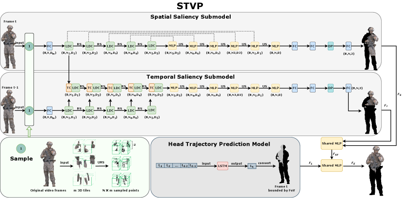
When drawn by conspicuous geometric shapes, vivid colors, or moving objects, a user will cast his or her view to that specific region by slowly changing his or her trajectory. Based on this intuition, we develop STVP, consisting of two main models: a saliency detection model and a user head trajectory prediction model, where the saliency detection model is subdivided into temporal saliency and spatial saliency detection in order to identify spatial and temporal salient regions, respectively. The detailed structure of STVP is shown in Fig. 2. The approximate principles of the saliency model and the trajectory prediction model are described in the following.
Prerequisites: To ensure the performance of saliency detection, we have to make the sampling results of adjacent frames similar in the time dimension to preserve temporal information and make the sampling points aggregated in local space to preserve spatial information. Furthermore, due to the large amount of point cloud video data, an effective sampling method is crucial. Addressing this issue, we propose a saliency detection model that incorporates a tile-based URS unit.
Input: Assuming there are frames in a point cloud video, and points in frame , representing the 3D scene.
Given consecutive 3D point cloud frames, we extract spatial features in the current frame and capture temporal features between consecutive frames in spatial-temporal saliency detection sub-model. In addition, the user’s head state records before time are input to the trajectory prediction model to predict the head state of the current frame , where the user’s head state at time is composed of the head coordinates and the Euler angles of the head rotation , i.e., , .
Saliency detection: To reduce computation power consumption and improve processing efficiency, original video frames are sampled through the URS unit before being fed into the temporal and spatial saliency detection sub-models in parallel. Then we propose an LDC module, which catches local color and coordinate discrepancies, to learn spatial saliency features and a 3D tile-based TC layer to learn temporal saliency features . The details of saliency detection model are explained in Section IV.
Head trajectory prediction and feature fusion:
To predict the user’s head state of frame , we use LSTM to analyze the patterns between historical trajectories. Then the predicted result is transformed into trajectory features by assigning different color attributes to the points inside and outside of the viewport.
In order to achieve accurate viewport prediction, we incorporate the results of saliency detection with those of trajectory prediction through an adaptive fusion process. The adaptive fusion of spatial-temporal saliency features , and trajectory features employs an attention mechanism to produce viewport prediction estimates . Further elaboration on the head trajectory prediction and feature fusion can be found in Section V.
IV Spatial-temporal saliency detection model
In this section, we will introduce the URS unit, the spatial saliency detection sub-model, and the temporal saliency detection sub-model.
IV-A Uniform-Random Sampling
Reducing the number of points in a point cloud video through sampling offers benefits like decreased computation and communication consumption. The URS method is proposed for effective uniformly spaced sampling, preserving temporal information, and KNN is used to aggregate spatial information from neighboring points.
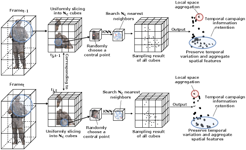
Assuming the total number of each frame is , each frame is cut into 3D tiles in the spatial dimension for transmission. Let be the -th 3D tile in frame , the total number of sampling points is and let be the -th 3D tile in frame and be the sampled data of 3D tile in frame .
As illustrated in Fig. 3, we establish a mapping relationship between 3D tiles, and , as they share similar spatial locations in their respective frames. This mapping is crucial for the TC layer to analyze changes in global information at their corresponding locations. To ensure the preservation of temporal information, we evenly distribute sampling points within mapping 3D tiles to guarantee similar sampling results. For efficient sampling, we further divide each 3D tile into (ranging from 10 to ) smaller cubes and randomly select central points. Around these central points, we search for neighbors as sampling points using KNN to consolidate local spatial information, where , and is the total number of sampling points in each 3D tile. With the introduced URS method, we can adeptly choose evenly spaced sampling points to retain temporal information. Furthermore, the URS sampling process leverages random sampling, providing an additional boost to sampling efficiency. The overall time complexity of URS is , so VS and URS exhibits lower time complexity compared to FPS. To further compare the fastness of VS and URS, we conduct full experiments in Sec.VI.
The implementation of TC layer requires that sampled data with similar spatial locations have a close mapping relationship. The degree of this closeness can be estimated by the proposed inter-frame mapping strength in Sec.VI, which measures the level of temporal information retention.
IV-B Spatial Saliency Detection Sub-model
The sampling result of frame obtained by URS is passed to the Fully Connected (FC) layer for feature extraction, to the LDC module for spacial encoding and to the RS layer for down-sampling.
Given the coordinate attributes and color attributes of each point in , we firstly obtain the initial feature of point through the FC layer, the process of feature extraction is simply expressed as:
| (1) |
where denotes concatenation. Finally, the sampled data goes through the FC layer to obtain the initial features . Then we further use LDC to fully integrate local coordinate and color discrepancies. The key components of LDC are divided into three parts: Neighborhood Coding, Attention Pooling and Dilated Residual Blocks.
Neighborhood Coding. This Neighborhood Coding unit explicitly embeds the coordinate and color discrepancies between each point in and its all neighboring points. In this way, the corresponding point features are always aware of their relative spatial differences, facilitating the network’s ability to learn spatial salient features more effectively.
For the coordinate and color attributes , of neighboring point around the point , where , is the set of color attributes of neighboring point , we explicitly encode the relative discrepancies as follows:
| (2) |
| (3) |
| (4) |
where the constants , and are used in the luminance algorithm[45] to convert RGB values to grayscale , taking into account the sensitivity of the human eye to red, green, and blue. denotes the coordinate relative Euclidean distance.
The discrepancy encoding between point and neighboring point is correspondingly connected with the initial feature to obtain the enhanced point feature . Then a set of enhanced features of point encoded with all neighboring points can be obtained through neighborhood coding.
Attention Pooling. This unit is used to aggregate each feature in the set of enhanced features as the spatial discrepancy feature of point . Thus each point contains the features of each neighboring point, which can compensate for the reduction of both temporal and spatial information, which is caused by the replacement of URS by RS as the downsampling technique in the following network training process.
Given each enhanced feature , we first use shared function to learn its attention score . Then we use function to normalize attention score , and weight enhanced feature by the normalized score to obtain the spatial discrepancy feature as follows:
| (5) |
| (6) |
where is the shared weight, is function, and means Shared MLP function.
Dilated Residual Blocks. The neighborhood coding and attention pooling can spatially link each sampled point to neighbors. To expand the receptive field of each point, we perform neighborhood coding and attention pooling twice in dilated residual blocks to receive information from up to neighbors.
According to the encoding process of the LDC module above, the process of passing the initial features of the sampled data through the -th LDC module and RS layer is simplified as:
| (7) |
| (8) |
where denotes the encoded features of through -th LDC and RS, which is passed to -th LDC module as input, and the input of st LDC module, , is initialized according to the Eq. 8. represents the -th LDC module, is the learnable weight, represents the -th RS layer.
The encoded features are decoded by applying MLP layers, Up-Sampling (US) layers, and FC layers. Additionally, to prevent overfitting, a Dropout (DP) layer is used. The output of this decoding process is a set of spatial saliency features, denoted by .
IV-C Temporal Saliency Detection Sub-model
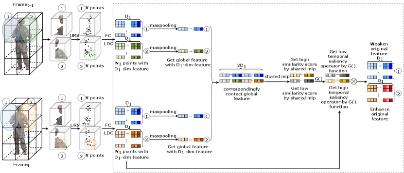
Based on the mapping relationship of and extracted from frame and , we propose a TC module to capture temporal information by comparing feature difference between them, as the feature difference can reflect the degree of variation from to .
The general structure of TC is shown in Fig. 4 and is explicitly expressed as follows:
Maxpooling. First, compute the global features of the two corresponding 3D tiles, and , separately:
| (9) |
| (10) |
where and denote the inputs of the -th TC from 3D tile and 3D tile , respectively. The and are initialized as the first encoded features and . and refer to the global features of and , respectively, computed through the function .
Comparing Feature Similarity. Compare the similarity of the corresponding global features, obtain the similarity score, and convert it into saliency intensity. It is defined as follows:
| (11) |
| (12) |
where denotes the similarity score calculated between the corresponding global features and . is the intensity of temporal saliency obtained by applying the temporal saliency operator, , on the similarity score . The operator is defined as . A lower degree of variation and a smaller are expected when the similarity score, , is higher between the global features and .
Weighting Features. Weighting input feature with saliency intensity. It is defined as follows:
| (13) |
| (14) |
where the temporal change features are obtained by weighting the input features , from frame , with the temporal saliency intensity. The minimum saliency intensity is 1. This means that if the saliency intensity is greater than 1, the saliency intensity will be superimposed after 5 TC layers, otherwise, it will always be 1, without changing the input features. After applying LDC and RS to it, the resulting features are passed as input to the next TC module.
With multiple TC modules, we can efficiently capture the temporal information between the mapping 3D tiles, and then we obtain the temporal salient features by decoding using MLP, US and FC layer.
V User’s Head Trajectory Prediction Module and Feature Fusion Unit
This section presents the LSTM-based module for predicting head trajectory and the feature fusion unit that utilizes attention mechanisms.
Because LSTM has the memory to learn the temporal dependence between observations, we use it to predict the user’s head state at the next moment based on the past user head position. The state update process of user’s head state ( is the time index) through the LSTM cell is shown in the following equation:
| (15) |
where is the hidden state of the LSTM cell structure at -th moments. is the nonlinear activation function of the LSTM cell. Each LSTM cell contains forget gate , input gate , output gate and cell state . The specific encoding process of LSTM cells is as follows:
| (16) |
| (17) |
| (18) |
| (19) |
| (20) |
| (21) |
where is the connection vector between the hidden layer state and the input . , , , are the learnable weights in the network and are the learnable biases in the network. denotes the function. Then hidden state and the next moment head state are passed into the next LSTM cell to learn the temporal dependence.
At the last LSTM cell, we get the predicted result of the user’s head state . The user’s predicted head state is projected onto the user’s viewport, and the current frame is divided into two regions based on its location relative to the viewport, as illustrated in Fig. 2. An RGB color scheme is assigned to the points inside and outside the viewport, where points within the viewport are colored white (RGB values of 255,255,255) while points outside the field of view (FoV) are colored black (RGB values of 0,0,0). After that, the features of the current frame are extracted as trajectory features .
Then, we need to integrate spatial saliency features and temporal saliency features into saliency features , and then integrate the saliency features with trajectory features to get final predicted estimates .
Traditional feature aggregation methods such as or lead to a significant loss of point information because they aggregate features without considering their relationships.
To avoid this loss, we use the attention mechanism to adaptively fuse the spatial-temporal saliency features of point cloud videos. The specific fusion process is as follows:
Computing attention scores. Given the spatial saliency features and the temporal saliency features , we use the shared MLP followed by function to calculate the attention scores. It is formally defined as follows:
| (22) |
| (23) |
where is the learnable weight, is the function, and is a proxy for shared MLP.
Weighting Features. The learned attention scores can be regarded as a mask for the automatic selection of salient features. The features are weighted to output the saliency feature , which is represented as follows:
| (24) |
where denotes the element-wise multiplication.
Second, we use the same fusion approach to fuse salient features with trajectory features :
| (25) |
| (26) |
| (27) |
where are the learnable weight parameters, is the function, is a proxy for shared MLP and denotes the element-wise multiplication. Finally, we get the viewport prediction features , which divides the points into points in the viewport and points outside the viewport.
VI Experiment
In this section, we verify the effectiveness of our proposed prediction method through extensive experiments.
VI-A Experimental Setup
VI-A1 Datasets
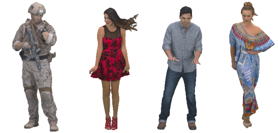
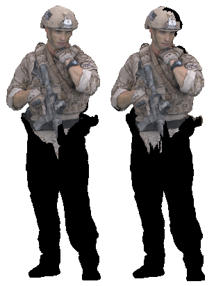
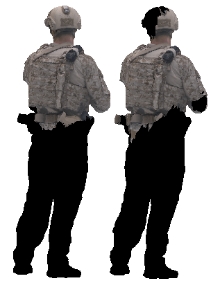
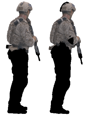
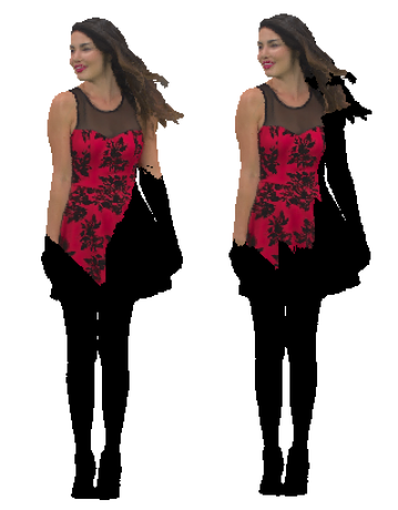
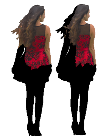
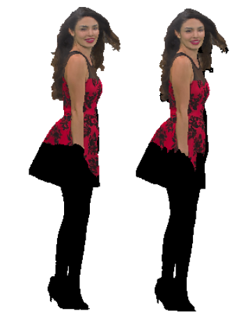
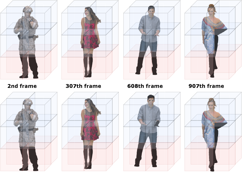
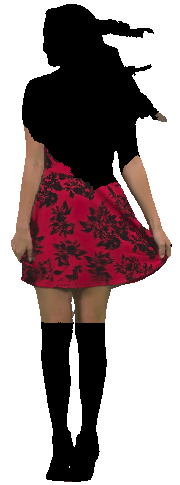
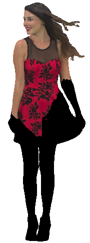
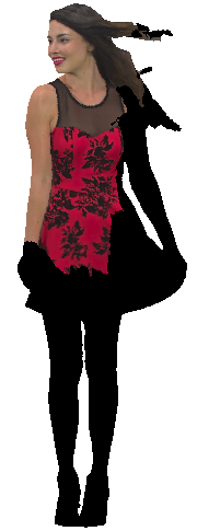
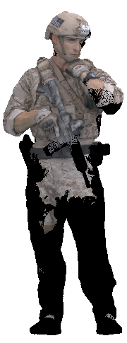
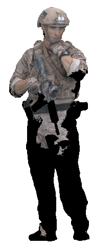
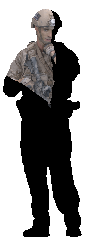
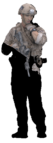
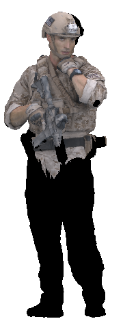
We choose four point cloud video sequences from the 8iVFB dataset [46], namely “Soldier”, “Redandblack”, “Loot”, and “Longdress”, as shown in Fig. 5. These sequences provide comprehensive coverage of the portrait characters’ entire body and allow users to observe their movements. During the model training phase, we allocate 900, 150, and 150 frames for training, validation, and testing, respectively. On three networks (STVP, RandLANet, BAAF-Net), we conduct experiments using 12, 20, and 36 3D tiles () to analyze the impact of varying the number of 3D tiles on viewport prediction.
We recruit 40 student volunteers (25 males and 15 females) for our experiment to view point cloud videos using HMDs. The experiment requires participants to experience a 6DoF immersive experience and explore areas of interest in a way they deem appropriate during the viewing process. The head trajectories of all participants are meticulously recorded throughout the entire duration of the video.
VI-A2 Implementation
Our STVP model has been implemented using TensorFlow, and we plan to make the experimental code publicly available on GitHub upon acceptance. The details of the network architecture are explained in Appendix. All experiments are conducted on our AI server equipped with four Nvidia Tesla V100 GPUs.
VI-A3 Metrics
We assess the overall performance of STVP using various metrics.
(1) Sampling performance: To evaluate the performance of our URS method, the memory consumption, time consumption and inter-frame mapping intensity (IFMI) are compared with other sampling competitors. To check the IFMI of different sampling methods, we propose a metric named as distance and color variation values (DaCVV). It calculates the coordinates and the degree of color difference between the point and point from the corresponding 3D tiles, and is defined as:
| (28) |
where the and are the max coordination and color distance of 3D tile , respectively.
Thus we can calculate the DaCVV between point from and point from . If the DaCVV between two points is less than a certain threshold, the two points are considered to be mapped to each other. We count the ratio of all mapped points to all sampled points as IFMI. We try to compare the IFMI of each sampling method for DaCVV thresholds of .
(2) Saliency detection: To assess the saliency detection performance of STVP, we compare its predicted saliency output with the ground truth and other competing models. The evaluation is carried out using four metrics: accuracy , precision, recall, and mean intersection over union (MIoU).
(3) Viewport prediction: We evaluate the viewport prediction performance of STVP using the same metrics used in saliency detection evaluation. In particular, we extend the MIoU metric into two categories for the viewport prediction evaluation: point-level MIoU and tile-level MIoU. Point-level MIoU measures the ratio of intersection and concatenation of point-level prediction results with the ground truth, while tile-level MIoU measures the ratio of intersection and concatenation of tile-level prediction results with the ground truth.
VI-A4 Baselines
We compare STVP with the competitors in terms of sampling and saliency detection respectively.
(1) Baselines for sampling: The performance of URS is compared with five commonly used competitors: FPS [16], GS, RS, IDIS [17], VS [18].
(2) Baselines for saliency detection : PointNet++ [16] RandLANet[47] and BAAF-Net[48] have excellent performance in saliency detection, and we compare the saliency detection performance of STVP saliency detection network (STVP-SD) with them. Specifically, PointNet++ proposes a hierarchical ensemble abstraction method that takes a frame of point cloud image as input, and performs hierarchical downsampling and neighborhood group coding processes on each video frame, and the extracted spatial features contain more and more local information. Inspired by PointNet++, RandLANet improves the group encoding layer by creating a local feature aggregator to encode neighborhood coordination information, which can better learn spatial features. BAAF-Net goes one step further and proposes a bilateral context module to extend local coordinate encoding. The bilateral context module first fuses the local semantic context information of the point cloud frames into the local geometric context information and subsequently extracts local spatial features by adapting the local geometric context information to the local semantic context information.
VI-A5 Ablation setup
During the experiments, we also conduct the following ablation studies for STVP.
(12) RS++ and IDIS++: We replace URS of STVP with RS and IDIS, respectively, while keeping the STVP saliency extraction modules. This is to highlight the performance of the URS unit that can retain spatial-temporal information by comparison.
(3) LFA++: To demonstrate the potential benefits of using our proposed LDC, we replace LDC of STVP with LFA of RandLANet, which focuses only on the geometric coordinate information of the neighborhood. This allows us to better understand the performance of using the LDC, which leverages both the neighboring coordinate information and color information to obtain more accurate local spatial saliency, as explained in Sec. IV.
(4) TSD–: We remove the temporal saliency detection (TSD–) and obtain the viewport prediction results for this ablation experiment. By comparing the prediction results of STVP and TSD–, we obtain the importance of the temporal saliency model used to achieve the viewport prediction.
VI-B Experimental Results
The effect of the number of 3D tiles: We hypothesize that the number of 3D tiles can impact viewport prediction. In our experiments, as shown in Table II, varying the number of 3D tiles (12, 20, and 36) shows a slight increase in MIoU at both the point and tile-levels across different networks. However, the computation time for segmenting the entire point cloud video into individual 3D tiles significantly increases with the number. Therefore, for subsequent experiments, we set the number of 3D tiles to 12.
| Network | The number of 3D tiles | MIOU | slicing Time(s) | |
|---|---|---|---|---|
| point-level MIoU | tile-level MIoU | |||
| STVP | 12 | 82.09 | 88.10 | 300 |
| 20 | 82.67 | 89.03 | 420 | |
| 36 | 83.19 | 89.90 | 930 | |
| RandLA-Net | 12 | 61.66 | 74.32 | 289 |
| 20 | 62.36 | 75.15 | 315 | |
| 36 | 63.45 | 75.99 | 921 | |
| BAAF-Net | 12 | 64.66 | 77.29 | 275 |
| 20 | 65.97 | 78.06 | 422 | |
| 36 | 66.03 | 79.60 | 913 | |
| MIoU | Accuracy | Precision | Recall | ||
| Point-level MIoU | tile-level MIoU | ||||
| PointNet++ | 52.22 | - | 69.44 | - | - |
| RandLANet | 61.66 | 74.32 | 76.28 | 67.68 | 87.49 |
| BAAF-Net | 64.66 | 77.29 | 72.35 | 71.86 | 93.71 |
| STVP-SD | 71.82 | - | 84.30 | 88.45 | 72.64 |
| STVP | 82.09 | 88.10 | 90.17 | 83.72 | 96.80 |
| RS++ | 58.19 | 69.86 | 74.06 | 69.39 | 80.84 |
| IDIS++ | 59.40 | 70.90 | 79.12 | 78.12 | 79.53 |
| LFA++ | 61.38 | 77.50 | 77.32 | 81.02 | 61.05 |
| TSD– | 67.40 | 79.97 | 80.95 | 81.70 | 71.22 |
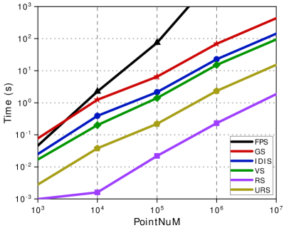
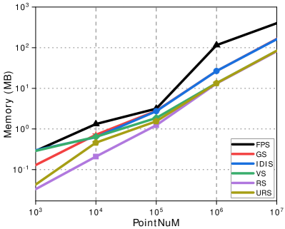
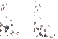
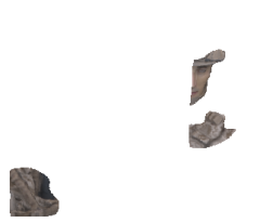
The efficiency of URS: To evaluate the efficiency of sampling, we select four levels of point cloud sizes ( points, points, points, points, and points). We downsample the point clouds to 1/4 of the original number of points using FPS, VS, IDIS, GS, RS, and URS, respectively. We measure the sampling time and memory consumption of each sampling method. Each sampling experiment is independently run 50 times, and the results are averaged for the final experimental results. Additionally, we present the sampling distribution results for each sampling method separately.
The time and memory consumption of all the sampling methods are listed in Fig.6. Experimental results indicate that the sampling time and memory consumption for URS is second only to RS, due to the fact that URS needs to slice the point cloud into 3D tiles and cubes. When the number of sampling points exceeds , the memory consumption of URS, VS and RS is much smaller than other sampling methods. The confidence intervals for this sampling comparison experiment at the 0.95 confidence level are shown in the Table IV.
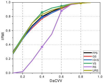
As shown in Fig. 6c, we also compare the IFMI of the six sampling methods at the same DaCVV values. When the DaCVV of URS are 0.3 and 0.8, its IFMI values are comparable to VS. In other cases, the IFMI values of URS are slightly lower than VS but higher than or equivalent to FPS, RS, GS and IDIS across all DaCVV values. However, considering time consumption, as shown in Fig. 6a, when the number of points in the point cloud is around , the time consumption of VS is 80 seconds higher than that of URS (while the number of points in a single frame ranges from to , and a point cloud video sequence contains a total of 300 frames). URS achieves efficient sampling efficiency by trading off a slight loss in temporal information retention.
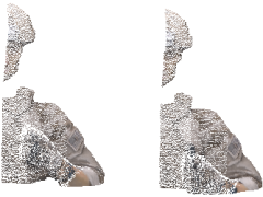
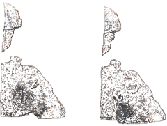
To observe the sampling effect visually, we take the corresponding 3D tiles and of consecutive frames and as sampling inputs and the number of sampling points is set to 12288 to get the result shown as Fig. 7. The sampling result shows that URS can indeed retain temporal information and spatial information. Although FPS and VS retain the temporal information between frames more completely, they consume more sampling time and sampling memory than URS and neglect spatial local information. RS and GS are even less preserving of temporal information than URS.
| Number of Points | Sampling Methods |
|
Mean | Sampling Methods |
|
Mean | Sampling Methods |
|
Mean | |||||||||
|---|---|---|---|---|---|---|---|---|---|---|---|---|---|---|---|---|---|---|
| FPS | Time(s) | [0.045,0.063] | 0.046 | VS | Time(s) | [0.016,0.019] | 0.017 | IDIS | Time(s) | [0.024,0.026] | 0.025 | |||||||
| Memory(MB) | [0.26,0.31] | 0.29 | Memory(MB) | [0.27,0.31] | 0.29 | Memory(MB) | [0.29,0.35] | 0.30 | ||||||||||
| Time(s) | [2.21,2.32] | 2.24 | Time(s) | [0.20,0.21] | 0.20 | Time(s) | [0.39,0.40] | 0.39 | ||||||||||
| Memory(MB) | [1.32,1.37] | 1.33 | Memory(MB) | [0.63,0.66] | 0.64 | Memory(MB) | [0.57,0.75] | 0.63 | ||||||||||
| Time(s) | [73.81,75.35] | 74.58 | Time(s) | [1.38,1.41] | 1.40 | Time(s) | [2.12,2.15] | 2.14 | ||||||||||
| Memory(MB) | [2.73,3.57] | 3.16 | Memory(MB) | [1.52,2.20] | 1.87 | Memory(MB) | [2.64,2.85] | 2.74 | ||||||||||
| Time(s) | [9917.09,9995.40] | 9956.25 | Time(s) | [15.04,15.20] | 15.12 | Time(s) | [22.64,22.81] | 22.73 | ||||||||||
| Memory(MB) | [114.40,116.83] | 115.61 | Memory(MB) | [13.43,13.57] | 13.50 | Memory(MB) | [26.52,26.86] | 26.70 | ||||||||||
| Time(s) | [358771.65,366392.56] | 362582.11 | Time(s) | [93.13,94.76] | 93.95 | Time(s) | [141.93,143.42] | 142.68 | ||||||||||
| Memory(MB) | [240.38,269.67] | 254.36 | Memory(MB) | [83.99,84.73] | 84.36 | Memory(MB) | [161.44,162.82] | 162.13 | ||||||||||
| GS | Time(s) | [0.074,0.079] | 0.077 | RS | Time(s) | [0.00097,0.00099] | 0.00097 | URS | Time(s) | [0.0028,0.0029] | 0.0028 | |||||||
| Memory(MB) | [0.11,0.13] | 0.13 | Memory(MB) | [0.026,0.039] | 0.033 | Memory(MB) | [0.026,0.045] | 0.043 | ||||||||||
| Time(s) | [1.22,1.26] | 1.24 | Time(s) | [0.0012,0.0019] | 0.0016 | Time(s) | [0.038,0.039] | 0.038 | ||||||||||
| Memory(MB) | [0.62,0.82] | 0.72 | Memory(MB) | [0.18,0.24] | 0.21 | Memory(MB) | [0.37,0.55] | 0.46 | ||||||||||
| Time(s) | [6.45,6.57] | 6.51 | Time(s) | [0.021,0.023] | 0.022 | Time(s) | [0.21,0.23] | 0.22 | ||||||||||
| Memory(MB) | [2.68,2.89] | 2.79 | Memory(MB) | [1.47,1.63] | 1.10 | Memory(MB) | [1.17,1.31] | 1.24 | ||||||||||
| Time(s) | [68.77,69.65] | 69.21 | Time(s) | [0.23,0.24] | 0.23 | Time(s) | [2.33,2.34] | 2.34 | ||||||||||
| Memory(MB) | [26.54,26.71] | 26.62 | Memory(MB) | [13.07,13.14] | 13.11 | Memory(MB) | [13.35,13.41] | 13.38 | ||||||||||
| Time(s) | [430.93,438.10] | 434.52 | Time(s) | [1.85,1.88] | 1.86 | Time(s) | [15.17,15.39] | 15.28 | ||||||||||
| Memory(MB) | [163.86,165.19] | 164.53 | Memory(MB) | [81.29,81.75] | 81.52 | Memory(MB) | [83.90,84.51] | 84.21 | ||||||||||

The results of saliency detection: We compare the saliency prediction performance of STVP-SD with PointNet++, BAFF, and RandLANet. The experimental results are shown in Table III, STVP-SD achieves on-par or better saliency detection performance than state-of-the-art methods. This is because STVP-SD makes full use of the temporal information, spatial coordinates and color information between point cloud video frames. Of the four performance metrics, STVP-SD is lower than the other three networks only in the metric of recall, due to the overly stringent conditions for determining the visible region.
The results of viewport prediction: Table III presents the experimental results, showing that STVP achieved high viewport prediction performance, with a point-level MIoU of 82.09%. The accuracy at the tile-level is even higher, with an MIoU of 88.10%.
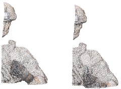
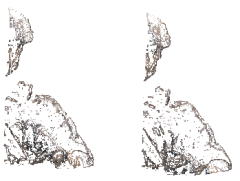
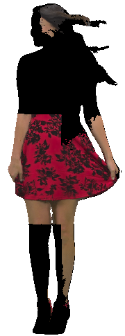
To visualize the prediction results, we extract one frame from two video sequences to display the final viewport prediction results. The prediction results are presented in two forms: a point-level prediction (Fig. 8) and a tile-level prediction (Fig. 9). From the point-level prediction results, we can see that although the STVP predictions are slightly different at the edge of the viewport compared to the ground truth, their viewport ranges largely overlap. However, their viewport edges do not resemble this defect, which is perfectly solved by extending the predictions to the tile level. From the tile-level prediction results, we can see that ground truth is almost the same as the predicted result.
The result of ablation: We also compare the performance of all ablation networks, and show the results in Table III. The result indicates that substituting the URS unit with either RS or IDIS leads to a reduction of approximately 23% in the MIoU score of the prediction outcome. This shows that URS plays a fundamental role in preserving the information of the original point cloud video. Replacing or removing it has a large impact on the viewport prediction. The LDC replacement also has a large impact on prediction performance. This is because both spatial color and geometric prominence attract the user’s attention, and LDC increases color discrepancy coding compared to LFA, which can effectively capture spatially color salient regions and fully improve the spatial saliency prediction performance.
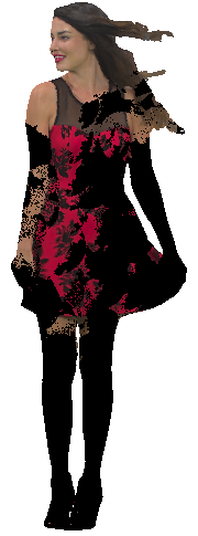
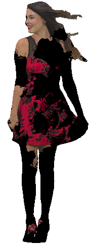
We also visualize the prediction results of the ablation experiments in Fig. 10. Since RS does not guarantee that the sampling results of adjacent video frames match, RS++ leads to disconnected frames within the viewport in the prediction results as shown in Fig. 10a and Fig. 10g. Due to the low degree of local spatial information retention in IDIS, IDIS++ also leads to the above situation, as shown in Fig. 10b and Fig. 10h. Meanwhile, since LFA ignores spatially salient information, from Fig. 10c and Fig. 10i we can see that the results of LFA++ have a salient part of the region less than the ground truth, e.g., hair in “Redandblack” and gun in “Soldier”. The temporal detection sub-module is created to capture the dynamic saliency region between frames. Therefore, as shown in Fig. 10d and Fig. 10j, the result of TSD– lacks some dynamic salient regions, e.g., hair in “Redandblack”, neck in “Soldier”, compared with the ground truth.
VII Conclusion
This paper proposes a high-precision viewport prediction scheme for point cloud video exploring viewport trajectory and video saliency information. In particular, we propose a novel and efficient sampling method, and a new saliency detection method incorporating temporal and spatial information to capture dynamic, static geometric, and color salient regions. Our proposal smartly fuses the saliency and trajectory information to achieve more accurate viewport prediction. We have conducted extensive simulations to evaluate the efficacy of our proposed viewport prediction methods using state-of-the-art point cloud video sequences. The experimental results demonstrate the superiority of the proposal over existing schemes.
ACKNOWLEDGMENT
This work is supported in part by grants from the National Natural Science Foundation of China (52077049), the Anhui Provincial Natural Science Foundation (2008085UD04)
References
- [1] D. Mieloch, P. Garus, M. Milovanović, J. Jung, J. Y. Jeong, S. L. Ravi, and B. Salahieh, “Overview and efficiency of decoder-side depth estimation in mpeg immersive video,” IEEE Transactions on Circuits and Systems for Video Technology, vol. 32, no. 9, pp. 6360–6374, 2022.
- [2] R. Mekuria, K. Blom, and P. Cesar, “Design, implementation, and evaluation of a point cloud codec for tele-immersive video,” IEEE Transactions on Circuits and Systems for Video Technology, vol. 27, no. 4, pp. 828–842, 2016.
- [3] Z. Liu, Q. Li, X. Chen, C. Wu, S. Ishihara, J. Li, and Y. Ji, “Point cloud video streaming: Challenges and solutions,” IEEE Network, vol. 35, no. 5, pp. 202–209, 2021.
- [4] B. Han, Y. Liu, and F. Qian, “Vivo: Visibility-aware mobile volumetric video streaming,” in Proceedings of the 26th Annual International Conference on Mobile Computing and Networking, ser. MobiCom ’20. New York, NY, USA: Association for Computing Machinery, 2020.
- [5] T. Stockhammer, “Dynamic adaptive streaming over http –: Standards and design principles,” in Proceedings of the Second Annual ACM Conference on Multimedia Systems, ser. MMSys ’11. New York, NY, USA: Association for Computing Machinery, 2011, p. 133–144.
- [6] J. Li, C. Zhang, Z. Liu, R. Hong, and H. Hu, “Optimal volumetric video streaming with hybrid saliency based tiling,” IEEE Transactions on Multimedia, 2022.
- [7] X. Hou and S. Dey, “Motion prediction and pre-rendering at the edge to enable ultra-low latency mobile 6dof experiences,” IEEE Open Journal of the Communications Society, vol. 1, pp. 1674–1690, 2020.
- [8] Z. Wang, Z. Zhou, H. Lu, Q. Hu, and J. Jiang, “Video saliency prediction via joint discrimination and local consistency,” IEEE Transactions on Cybernetics, vol. 52, no. 3, pp. 1490–1501, 2022.
- [9] W. Wang, J. Shen, F. Guo, M.-M. Cheng, and A. Borji, “Revisiting video saliency: A large-scale benchmark and a new model,” in 2018 IEEE/CVF Conference on Computer Vision and Pattern Recognition, 2018, pp. 4894–4903.
- [10] Y. Zhu, G. Zhai, Y. Yang, H. Duan, X. Min, and X. Yang, “Viewing behavior supported visual saliency predictor for 360 degree videos,” IEEE Transactions on Circuits and Systems for Video Technology, vol. 32, no. 7, pp. 4188–4201, 2022.
- [11] M. Paul and M. Musfequs Salehin, “Spatial and motion saliency prediction method using eye tracker data for video summarization,” IEEE Transactions on Circuits and Systems for Video Technology, vol. 29, no. 6, pp. 1856–1867, 2019.
- [12] C. Chen, M. Ye, M. Qi, J. Wu, Y. Liu, and J. Jiang, “Saliency and granularity: Discovering temporal coherence for video-based person re-identification,” IEEE Transactions on Circuits and Systems for Video Technology, vol. 32, no. 9, pp. 6100–6112, 2022.
- [13] A. Nguyen, Z. Yan, and K. Nahrstedt, “Your attention is unique: Detecting 360-degree video saliency in head-mounted display for head movement prediction,” in Proceedings of the 26th ACM International Conference on Multimedia, ser. MM ’18. New York, NY, USA: Association for Computing Machinery, 2018, p. 1190–1198.
- [14] X. Zhang, G. Cheung, Y. Zhao, P. Le Callet, C. Lin, and J. Z. G. Tan, “Graph learning based head movement prediction for interactive 360 video streaming,” IEEE Transactions on Image Processing, vol. 30, pp. 4622–4636, 2021.
- [15] Y. Bao, H. Wu, T. Zhang, A. A. Ramli, and X. Liu, “Shooting a moving target: Motion-prediction-based transmission for 360-degree videos,” in 2016 IEEE International Conference on Big Data (Big Data), 2016, pp. 1161–1170.
- [16] C. R. Qi, L. Yi, H. Su, and L. J. Guibas, “Pointnet++: Deep hierarchical feature learning on point sets in a metric space,” in Proceedings of the 31st International Conference on Neural Information Processing Systems, ser. NIPS’17. Red Hook, NY, USA: Curran Associates Inc., 2017, p. 5105–5114.
- [17] F. Groh, P. Wieschollek, and H. P. A. Lensch, Flex-Convolution: Million-Scale Point-Cloud Learning Beyond Grid-Worlds. Computer Vision – ACCV 2018, 2019.
- [18] Y. Zhou and O. Tuzel, “Voxelnet: End-to-end learning for point cloud based 3d object detection,” in 2018 IEEE/CVF Conference on Computer Vision and Pattern Recognition, 2018, pp. 4490–4499.
- [19] F. Yin, Z. Huang, T. Chen, G. Luo, G. Yu, and B. Fu, “Dcnet: Large-scale point cloud semantic segmentation with discriminative and efficient feature aggregation,” IEEE Transactions on Circuits and Systems for Video Technology, vol. 33, no. 8, pp. 4083–4095, 2023.
- [20] J. Li, B. M. Chen, and G. H. Lee, “So-net: Self-organizing network for point cloud analysis,” in 2018 IEEE/CVF Conference on Computer Vision and Pattern Recognition, 2018, pp. 9397–9406.
- [21] H. Zhao, L. Jiang, C.-W. Fu, and J. Jia, “Pointweb: Enhancing local neighborhood features for point cloud processing,” in 2019 IEEE/CVF Conference on Computer Vision and Pattern Recognition (CVPR), 2019, pp. 5560–5568.
- [22] L. Wang, Y. Huang, Y. Hou, S. Zhang, and J. Shan, “Graph attention convolution for point cloud semantic segmentation,” in 2019 IEEE/CVF Conference on Computer Vision and Pattern Recognition (CVPR), 2019, pp. 10 288–10 297.
- [23] F. Qian, L. Ji, B. Han, and V. Gopalakrishnan, “Optimizing 360 video delivery over cellular networks,” in Proceedings of the 6th Workshop on All Things Cellular - Operations, Applications and Challenges, AllThingsCellular@MobiCom 2016, New York City, New York, USA, October 3-7, 2016, M. K. Marina and U. C. Kozat, Eds. ACM, 2016, pp. 1–6.
- [24] Y. Ban, L. Xie, Z. Xu, X. Zhang, Z. Guo, and Y. Wang, “Cub360: Exploiting cross-users behaviors for viewport prediction in 360 video adaptive streaming,” in 2018 IEEE International Conference on Multimedia and Expo (ICME), 2018, pp. 1–6.
- [25] C.-L. Fan, J. Lee, W.-C. Lo, C.-Y. Huang, K.-T. Chen, and C.-H. Hsu, “Fixation prediction for 360° video streaming in head-mounted virtual reality,” in Proceedings of the 27th Workshop on Network and Operating Systems Support for Digital Audio and Video, ser. NOSSDAV’17. New York, NY, USA: Association for Computing Machinery, 2017, p. 67–72.
- [26] L. Xie, Z. Xu, Y. Ban, X. Zhang, and Z. Guo, “360probdash: Improving qoe of 360 video streaming using tile-based http adaptive streaming,” in Proceedings of the 25th ACM International Conference on Multimedia, ser. MM ’17. New York, NY, USA: Association for Computing Machinery, 2017, p. 315–323.
- [27] Y. S. de la Fuente, G. S. Bhullar, R. Skupin, C. Hellge, and T. Schierl, “Delay impact on mpeg omaf’s tile-based viewport-dependent 360° video streaming,” IEEE Journal on Emerging and Selected Topics in Circuits and Systems, vol. 9, no. 1, pp. 18–28, 2019.
- [28] S. Gül, D. Podborski, T. Buchholz, T. Schierl, and C. Hellge, “Low-latency cloud-based volumetric video streaming using head motion prediction,” in Proceedings of the 30th ACM Workshop on Network and Operating Systems Support for Digital Audio and Video, ser. NOSSDAV ’20. New York, NY, USA: Association for Computing Machinery, 2020, p. 27–33. [Online]. Available: https://doi.org/10.1145/3386290.3396933
- [29] S. Yoon, H. j. Lim, J. H. Kim, H.-S. Lee, Y.-T. Kim, and S. Sull, “Deep 6-dof head motion prediction for latency in lightweight augmented reality glasses,” in 2022 IEEE International Conference on Consumer Electronics (ICCE), 2022, pp. 1–6.
- [30] J. Li, L. Han, C. Zhang, Q. Li, and Z. Liu, “Spherical convolution empowered viewport prediction in 360 video multicast with limited fov feedback,” ACM Transactions on Multimedia Computing, Communications, and Applications (TOMM), 2022.
- [31] L. Itti, C. Koch, and E. Niebur, “A model of saliency-based visual attention for rapid scene analysis,” IEEE Transactions on Pattern Analysis and Machine Intelligence, vol. 20, no. 11, pp. 1254–1259, 1998.
- [32] T. Judd, K. Ehinger, F. Durand, and A. Torralba, “Learning to predict where humans look,” in 2009 IEEE 12th International Conference on Computer Vision, 2009, pp. 2106–2113.
- [33] R. Cong, J. Lei, H. Fu, M.-M. Cheng, W. Lin, and Q. Huang, “Review of visual saliency detection with comprehensive information,” IEEE Transactions on Circuits and Systems for Video Technology, vol. 29, no. 10, pp. 2941–2959, 2019.
- [34] Q. Lai, T. Zhou, S. Khan, H. Sun, J. Shen, and L. Shao, “Weakly supervised visual saliency prediction,” IEEE Transactions on Image Processing, vol. 31, pp. 3111–3124, 2022.
- [35] M. Zhong and L. Shen, “Learning to predict what humans look at: Computational visual attention model for specific category,” in 2022 International Symposium on Electrical, Electronics and Information Engineering (ISEEIE), 2022, pp. 1–7.
- [36] G. Ma, S. Li, C. Chen, A. Hao, and H. Qin, “Rethinking image salient object detection: Object-level semantic saliency reranking first, pixelwise saliency refinement later,” IEEE Transactions on Image Processing, vol. 30, pp. 4238–4252, 2021.
- [37] V. F. Figueiredo, G. L. Sandri, R. L. de Queiroz, and P. A. Chou, “Saliency maps for point clouds,” in 2020 IEEE 22nd International Workshop on Multimedia Signal Processing (MMSP), 2020, pp. 1–5.
- [38] X. Ding, W. Lin, Z. Chen, and X. Zhang, “Point cloud saliency detection by local and global feature fusion,” IEEE Transactions on Image Processing, vol. 28, no. 11, pp. 5379–5393, 2019.
- [39] K. Zhang and Z. Chen, “Video saliency prediction based on spatial-temporal two-stream network,” IEEE Transactions on Circuits and Systems for Video Technology, vol. 29, no. 12, pp. 3544–3557, 2019.
- [40] Z. Wu, L. Su, and Q. Huang, “Learning coupled convolutional networks fusion for video saliency prediction,” IEEE Transactions on Circuits and Systems for Video Technology, vol. 29, no. 10, pp. 2960–2971, 2019.
- [41] L. Zhao and W. Tao, “Jsnet++: Dynamic filters and pointwise correlation for 3d point cloud instance and semantic segmentation,” IEEE Transactions on Circuits and Systems for Video Technology, vol. 33, no. 4, pp. 1854–1867, 2023.
- [42] A. Behl, D. Paschalidou, S. Donné, and A. Geiger, “Pointflownet: Learning representations for rigid motion estimation from point clouds,” in 2019 IEEE/CVF Conference on Computer Vision and Pattern Recognition (CVPR), 2019, pp. 7954–7963.
- [43] X. Liu, C. R. Qi, and L. J. Guibas, “Flownet3d: Learning scene flow in 3d point clouds,” CVPR, 2019.
- [44] G. Wang, X. Wu, Z. Liu, and H. Wang, “Hierarchical attention learning of scene flow in 3d point clouds,” IEEE Transactions on Image Processing, vol. 30, pp. 5168–5181, 2021.
- [45] W. K. Pratt, Digital Image Processing (2nd Ed). Digital image processing (2nd ed.), 1987.
- [46] E. d’Eon, B. Harrison, T. Myers, and P. Chou, “8i voxelized full bodies—a voxelized point cloud dataset, document iso,” IEC JTC1/SC29 Joint WG11/WG1 (MPEG/JPEG), WG11M40059/WG1M74006, Geneva, 2017.
- [47] Q. Hu, B. Yang, L. Xie, S. Rosa, Y. Guo, Z. Wang, N. Trigoni, and A. Markham, “Randla-net: Efficient semantic segmentation of large-scale point clouds,” in 2020 IEEE/CVF Conference on Computer Vision and Pattern Recognition (CVPR), 2020, pp. 11 105–11 114.
- [48] S. Qiu, S. Anwar, and N. Barnes, “Semantic segmentation for real point cloud scenes via bilateral augmentation and adaptive fusion,” in 2021 IEEE/CVF Conference on Computer Vision and Pattern Recognition (CVPR), 2021, pp. 1757–1767.