Viscous shocks and long-time behavior of scalar conservation laws
Abstract
We study the long-time behavior of scalar viscous conservation laws via the structure of -limit sets. We show that -limit sets always contain constants or shocks by establishing convergence to shocks for arbitrary monotone initial data. In the particular case of Burgers’ equation, we review and refine results that parametrize entire solutions in terms of probability measures, and we construct initial data for which the -limit set is not reduced to the translates of a single shock. Finally we propose several open problems related to the description of long-time dynamics.
1 Introduction and main results
We are interested in the long-time dynamics of viscous scalar conservation laws,
| (1.1) |
with smooth and strictly convex flux function , that is, for all . A typical example is Burgers’ equation where . The Cauchy problem for (1.1) is globally well-posed in the space , see e.g. [29]. More precisely, given initial data , equation (1.1) has a unique global solution such that converges to in the weak- topology of as . By parabolic regularity, the function is smooth for all positive times. For any , let be the nonlinear map defined by , where is the solution of (1.1) with initial data . We also write , the identity map.
To a first approximation, the long-time behavior of as is described by the collection of all limit points, usually referred to as the -limit set. The unboundedness of the spatial domain implies a typical lack of compactness of the trajectory , and the -limit set may indeed be empty when convergence is measured in the uniform topology defined by the norm in . It is therefore preferable to rely on the local topology induced by , which is the topology of uniform convergence on compact intervals . The -limit set is commonly defined as follows:
| (1.2) |
but this definition assigns a particular role to the laboratory frame and is not invariant under Galilean transformations. A somewhat richer description of asymptotic behavior is obtained by considering the set of limit points modulo translations,
| (1.3) |
where . Note that we use the zero subscript in the definition of in (1.2) to emphasize the fixed origin in the definition of locally uniform convergence in (1.2).
Fairly standard results assert that both and are non-empty, compact, connected, fully invariant, attractive, and chain recurrent (up to translations) in the topology of ; see Propositions 3.2 and 3.3. Full invariance implies in particular that for any in the -limit set, there exists a solution of (1.1) that is defined for all and satisfies . We refer to such solutions, defined for all positive and negative times, as entire solutions. Describing all possible long-term dynamics can then be rephrased as describing all subsets of the family of entire solutions that can occur as -limit sets for bounded initial data.
The results we present can be seen as small steps in this direction. Somewhat trivial candidates for the -limit sets are first spatially constant states and then viscous shocks, found as traveling-wave solutions with , for all , and given by the Rankine-Hugoniot formula . It is known since the classical work of Il’in and Oleinik [15] that large sets of initial data give rise to solutions of (1.1) that converge uniformly to shocks as , see also [8]. In Proposition 4.1 below, we show that this is the case for all initial data that are monotonically decreasing, without any assumption on the rate at which the limits are approached as . At this level of generality, we cannot prove convergence to a fixed translate of the shock as . In fact, as discussed in Remark 4.2, there exist monotone initial data with and such that, for instance, ; in particular one observes that for all .
Our first general result establishes a property reminiscent of the Poincaré-Bendixson theorem, in the sense that it describes the long-time behavior of solutions with initial data in -limit sets.
Proposition 1.1.
For every and any nonconstant , there exist real numbers such that
| (1.4) |
In particular, the set contains a shock unless it consists entirely of constants.
In other words, if is nonconstant, the -limit set consists of all translates of a viscous shock , together with the constant states and that arise as limits of the shock profile at . The proof relies on the simple observation that any such is necessarily monotonically decreasing, as a consequence of Oleinik’s inequality (2.2). We can thus invoke Proposition 4.1 to determine the -limit , which is included in since the latter set is invariant under the dynamics of (1.1).
Our remaining results focus on the specific case of Burgers’ equation, which through the Cole-Hopf transformation allows for a somewhat explicit representation of any solution in terms of its initial data. Interestingly, as pointed out in [16], bounded entire solutions of Burgers’ equation can be represented in terms of probability measures on the real line,
| (1.5) |
This remarkable formula gives, in particular, an explicit characterization of candidates for elements in -limit sets. In Section 5 we give a short proof of the representation (1.5), showing that the measure is unique and supported in the closure of the range of the entire solution . We also relate the measure to backward-in-time asymptotics of the entire solution . A striking result in this direction is:
Proposition 1.2.
Assume that is given by (1.5) for some probability measure on . A real number belongs to if and only if converges to in as .
It is also possible to determine the asymptotic behavior of as in Galilean frames with speeds . In that case we define
Proposition 1.3.
We refer to Propositions 5.6 and 5.8 below for more general statements, which also cover the somewhat delicate situation where . Other properties of the measure , such as the presence of atoms, can also be detected in the ancient behavior of the corresponding entire solution .
Lastly, we show that out of this plethora of entire solutions, the -limit set may contain elements that are not simply shocks or constants.
Proposition 1.4.
There exist initial data for Burgers’ equation such that contains a solution that is neither a constant nor a shock. In fact describes the merging of a pair of shocks into a single shock.
The construction is carried out in a somewhat explicit fashion in Section 6. In the terminology of dynamical systems, the -limit set contains a heteroclinic trajectory connecting the zero solution to a steady shock , as well as a continuous family of steady shocks interpolating between and . This can be compared to a famous example of coarsening dynamics due to Eckmann and Rougemont [5], also rigorously studied by Poláčik [21, 22], where the -limit set is a heteroclinic loop.
Outline. We recall basic properties of conservation laws and shocks in Section 2. We then formulate and establish properties of both -limit sets and in Section 3. Our first main result, the convergence to shocks for monotone initial data, is proved in Section 4. Section 5 derives the representation of entire solutions in terms of probability measures, displays some key examples, and relates measures to ancient limits. Lastly, Section 6 is devoted to the proof of Proposition 1.4. We conclude with a brief discussion.
Acknowledgements. This project started from discussions held in the stimulating atmosphere of the Mathematisches Forschungsinstitut Oberwolfach, in August 2021. ThG would like to thank Denis Serre for his expert advice on several points addressed in this work. The authors were partially supported by the grants ISDEEC ANR-16-CE40-0013 (ThG) and NSF DMS-1907391, DMS-2205663 (AS).
2 Properties of scalar conservation laws and shocks solutions
We first recall some basic properties of scalar conservation laws of the form (1.1).
A priori bounds and monotonicity.
The evolution semigroup defined by (1.1) in has the following properties :
-
a)
Monotonicity : if and almost everywhere, then everywhere when ;
-
b)
Contraction in : if satisfy , then and for all ;
-
c)
Conservation of mass : under the assumptions of b), we also have
Assertions a), b), c) are readily established using the parabolic maximum principle [24] and the fact that (1.1) is a conservation law, see e.g. [27, 29].
Another remarkable property of the solutions of (1.1) is a universal upper bound for the derivative , which is known as Oleinik’s inequality. Given , we define
| (2.1) |
Since constants are steady states of (1.1), monotonicity implies that the solution satisfies for all and all (in fact, due to the strong maximum principle, both inequalities are strict as soon as ). Oleinik’s inequality asserts that, for all and all ,
| (2.2) |
For convenience, we include a short proof of (2.2) in Section A.1.
Viscous shocks.
Given with , equation (1.1) has a unique traveling wave solution of the form , such that and , and . The profile is strictly decreasing and solves
| (2.3) |
where
| (2.4) |
Strict convexity of gives the Lax condition , and the ODE (2.3) then implies that converges exponentially to its limits at .
Stability of viscous shocks has been known since the classical work of Il’in and Oleinik [15]. For localized perturbations, that is, for initial data with for some , the solution of (1.1) converges uniformly to as , with as in (2.4) and
| (2.5) |
Extensions towards viscous conservation laws with more general flux function, allowing for degenerate shocks, can be found in the references [18, 8, 29, 20, 13, 11]. Rates of convergence can be obtained under stronger localization of the perturbations. However, the hypothesis that , which allows one to determine the asymptotic shift (2.5), seems to play an important role in all existing results. Our analysis in Section 4 removes this restriction for monotone solutions.
3 Properties of -limit sets
In this section we establish the properties of the -limit sets (1.2), (1.3) that were announced in the introduction. Here and in what follows, we denote by the distance on defined by
| (3.1) |
As is easily verified, on any bounded set , the topology defined by the distance (3.1) coincides with the topology of , namely the topology of uniform convergence on compact subsets of .
In view of the properties recalled in Section 2, for any initial data the solution of (1.1) belongs for all times to the ball
| (3.2) |
The following standard result plays a fundamental role:
Lemma 3.1.
When equipped with the topology of , the ball defined by (3.2) is closed and the solution map is continuous for any .
-
Proof . It is easy to check that is closed in , and the properties recalled in Section 2 imply that the semiflow maps the ball into itself. The key point is the continuous dependence of the solution upon the initial data , in the topology of . This a rather standard result for parabolic PDEs on unbounded domains, see e.g. [19]. For the reader’s convenience, the argument showing continuity is reproduced in Section A.2 below.
We are now in position to establish the main properties of the -limit set (1.2).
Proposition 3.2.
For any , the -limit set defined by (1.2) is bounded in and, when equipped with the topology of , has the following properties :
-
a)
is non-empty, compact, connected, and
(3.3) -
b)
is fully invariant, attractive, and chain recurrent, namely :
-
•
for all ;
-
•
for any neighborhood of , there exists such that for all ;
-
•
for each and any , there exists a closed -pseudo-orbit in starting at , that is, there exist finite sequences and for , such that and for all .
In particular, if , there exists an entire solution of (1.1) such that for all and ; moreover .
-
•
-
c)
is a bounded subset of for all , and any satisfies .
-
Proof . Smoothing properties of the parabolic equation (1.1) and a priori bounds for the solutions and their derivatives guarantee that, for any and any , the solution is uniformly bounded in for . This does not imply that the forward trajectory is compact in , because in general the map is not continuous at in that topology. However, for any , the trajectory is relatively compact and connected in . Topological properties (a) and dynamic properties (b) of the -limit set follow in a standard fashion. We include some details here for later reference.
1) Compactness and attractivity. It is easy to verify that the relation (3.3) is equivalent to the definition (1.2). Now (3.3) shows that is the intersection of a decreasing family of non-empty compact sets, so that is itself compact and non-empty. By the same argument, if is any neighborhood of in , there exists such that , which proves attractivity.
2) Connectedness. We argue by contradiction: if where are non-empty disjoint closed sets, then are in fact compact and are therefore separated by a distance . If are -neighborhoods of , respectively, then are non-empty disjoint open sets, and the attractivity property shows that, for sufficiently large, the connected forward orbit is contained in the neighborhood , without being included in either or , which is clearly impossible.
3) Full invariance. If there exists a sequence such that in . By Lemma 3.1, for any , we thus have
which proves that . Similarly, we can extract a subsequence (still denoted by ) such that , where satisfies . Altogether, this shows that for all . It is easy to deduce that, given any , there exists an entire solution of (1.1) such that .
4) Chain recurrence. This is a consequence of continuity and attractivity, which can be established as follows. Fix and take . By continuity, there exists such that, for all such that , one has for all . By attractivity, we can then choose such that for all . Now, we take such that , and also such that . For some , we define intermediate times such that and
Finally we denote for , and we take such that . Note that is given from the beginning, and we can take . We claim that the sequence for is the desired pseudo-orbit. Indeed for we have , hence
where we used the uniform continuity of and the fact that .
5) Assertion (c) is an easy consequence of parabolic smoothing and Oleinik’s inequality (2.2).
We next consider the larger -limit set (1.3), where limit points are considered up to translations in space. The analogue of Proposition 3.2 is:
Proposition 3.3.
For any , the -limit set defined by (1.3) is bounded in and, when equipped with the topology of , has the following properties :
-
a)
is non-empty, compact, connected, and
(3.4) -
b)
is fully invariant in time, translation invariant in space, uniformly attractive, and chain recurrent up to translations;
-
c)
is a bounded subset of for all , and any satisfies .
-
Proof . The proof is completely parallel to that of Proposition 3.2, and we just indicate here the main differences. The starting point is the formula (3.4), which is easily derived from the definition (1.3). Since the space-time trajectory is relatively compact in for any , we see that is non-empty and compact as the decreasing intersection of non-empty compact sets. Moreover, if is any neighborhood of in , we have for any sufficiently large , which means that attracts the trajectory uniformly in as . As a consequence, since the space-time trajectory is connected for all , the same argument as in Proposition 3.2 shows that is a connected set. There is no difference either in the reasoning showing that for all . Finally, the definition (1.3) immediately implies that for all , and the boundedness properties (c) are established exactly as before.
The main difference we would like to point out is that is not chain recurrent in the sense of Proposition 3.2, but only in a weaker sense that can be called “chain recurrence up to translations”. The precise definition is as follows: for each and any , there exist finite sequences , , and for , such that and for all . In other words, the definition of the -pseudo-orbit involves spatial shifts in addition to the time shifts , which is natural in view of (1.3). The existence of such a pseudo-orbit for all , all , and all is established by the same argument as in Proposition 3.2.
Although the -limit sets (1.2), (1.3) are relatively easy to define and enjoy the nice properties listed in Propositions 3.2 and 3.3, it is notoriously difficult to compute them for arbitrary initial data. In the case of equation (1.1), general results in this direction are only available under monotonicity assumptions. If is increasing, the solution remains increasing for all by the maximum principle, and as by Oleinik’s inequality (2.2). This implies that consists of the constant states for all , where are as in (2.1). On the other hand, if is decreasing, Proposition 4.1 below implies that is the set of all translates of the viscous shock , supplemented with the constant states and . A similar conclusion is reached if satisfies the assumptions of Il’in and Oleinik’s result [15]. Incidentally, we observe in this example that is a heteroclinic orbit in the terminology of dynamical systems, so that is not chain recurrent.
More generally, if and if there is a that is not a constant, then is decreasing by Proposition 3.3, and since we deduce that contains the translates of a viscous shock, as asserted in (1.4). So we see that Proposition 1.1 is a direct consequence of Propositions 3.3 and 4.1. In addition we have
Corollary 3.4.
For any , the -limit set contains a constant state or a viscous shock.
This statement can be compared with a result by S. Slijepčević and the first author [9] which shows that, for a general class of dissipative systems including reaction-diffusion equations on the real line, the -limit set of a bounded trajectory always contains an equilibrium. For the viscous conservation law (1.1), where all Galilean frames are equivalent, the role of equilibria is played by the constant states and the viscous shocks.
From a different perspective, one may wonder which collections of entire solutions of (1.1) may occur as -limit sets of bounded initial data. From the results presented thus far, only non-empty, compact, connected, invariant, and chain-recurrent sets are candidates. In general, compact, connected sets with a chain-recurrent flow are precisely the possible -limit sets of flows, in the sense that any such set is topologically conjugated to an -limit set of some flow [7]. It is however not clear at all if any compact, connected, invariant, and chain-recurrent set within the family of entire solutions is realized as the -limit set of the particular flow generated by the conservation law (1.1).
Remark 3.5.
In the definition (1.3) of the -limit set , we allow for arbitrary spatial shifts while the temporal shifts must go to infinity. This is clearly not the only possibility. One the one hand, we could restrict the class of spatial shifts by imposing, for instance, a Galilean constraint of the form with, typically, . Actually, we could even require that converges to some limit in as . In a different direction, we could consider all spatio-temporal shifts such that as , which potentially gives an -limit set even larger than (1.3). However, in the examples we are aware of, these alternative possibilities do not seem to change the nature of the -limit set in a profound way, so in what follows we stick to the original definition (1.3).
4 Convergence to shocks for monotone initial data
The main result of this section is:
Proposition 4.1.
Remark 4.2.
It is not difficult to find examples for which the shift function in (4.2) is not asymptotically linear, namely has no limit as . For instance, assume that but . Given any , we define for and for . As , monotonicity implies that for all . On the other hand, since , we can apply the result of [15] to deduce that converges uniformly to as , where
In particular one has by monotonicity. Now, taking taking , we see that by assumption on , and we conclude that as . A more explicit example of such a “sublinear shift” will be given in Section 5.2 below.
The remainder of this section is devoted to the proof of Proposition 4.1. Assume that the initial data are nonincreasing and satisfy (4.1) for some . The solution of (1.1) is smooth for positive times, and the strong maximum principle implies that for all and all . On the other hand, using for instance Lemma 3.1, it is not difficult to verify that the limits of as are independent of time. As a consequence, for each , there exists a unique point such that
| (4.3) |
Moreover is a smooth function of time thanks to the implicit function theorem.
Lemma 4.3.
The shift function defined by (4.3) satisfies
| (4.4) |
-
Proof . We use the monotonicity of the evolution map to compare the solution with suitably translated viscous shocks. Take small enough so that
(4.5) Since is nonincreasing and satisfies (4.1), there exist and such that
(4.6) where denotes the viscous shock connecting with . In fact, it is straightforward to verify that (4.6) holds as soon as and are sufficiently large, depending on . By monotonicity, we deduce from (4.6) that
(4.7) for all and all , where the speeds are given by the Rankine-Hugoniot formulas
(4.8) On the other hand, due to the second inequality in (4.5), there exist and such that
(4.9) In view of (4.9), we deduce from (4.7) that the shift function defined by (4.3) satisfies
(4.10) In particular we infer from (4.10) that
(4.11) Finally it is clear from (4.8) that as , which concludes the proof of (4.4).
In a second step, we consider the auxiliary function defined by
| (4.12) |
where the constants are defined in (2.4). This function is smooth for positive times and a direct calculation shows that it satisfies the evolution equation
| (4.13) |
The key step in the proof of Proposition 4.1 is :
Lemma 4.4.
The function defined by (4.12) converges uniformly to zero as :
| (4.14) |
-
Proof . Shifting the initial time if needed, we can assume without loss of generality that the functions and are smooth for all . We consider the linear advection-diffusion equation
(4.15) where the function is considered as given. The following – estimates are known for the solution of (4.15) with initial data :
(4.16) where is a universal constant. While the first bound in (4.16) is a direct consequence of the parabolic maximum principle, the second one takes into account the convexity of the flux function as well as the monotonicity of the solution . For the reader’s convenience, we provide a proof of the second estimate (4.16) in Section A.3.
For the time being, to conclude the proof of Lemma 4.4, we consider the solution of (4.13) with initial data . We know that because is decreasing and bounded, and that converges to zero as because of (2.4). As a consequence, given any , we can decompose , where and . For we denote by the solution of (4.15) with initial data , so that by linearity. Using (4.16), we infer that
so that . Since was arbitrary, this gives (4.14).
Equipped with Lemmas 4.3 and 4.4, it is now straightforward to conclude the proof of Proposition 4.1. Let be the convex function defined by , where are given by (2.4), and let
Fix any . In view of (4.12), the function defined by satisfies the ODE
This is to be compared with the ODE (2.3) satisfied by the viscous shock , namely and . If , we infer that . Integrating this differential inequality and recalling that , we obtain
| (4.17) |
Since by Lemma 4.14, it follows from (4.17) that converges to zero as , uniformly for in any compact interval. Taking into account the fact that both functions and are decreasing and have the same limits as , we deduce that the convergence is in fact uniform for all . This proves (4.2), and we already established in Lemma 4.3 that has a limit as .
Remark 4.5.
Neither the strict convexity of the flux nor the Lax condition for the shock is used in the proof of Proposition 4.1, which therefore remains valid if we only assume that for all .
5 Representation of entire solutions via probability measures
From now on we restrict our attention to the special case of Burgers’ equation
| (5.1) |
which corresponds to taking in (1.1). The Cauchy problem for (5.1) can be solved in explicit form through the celebrated Cole-Hopf transformation [4, 14]. As is easily verified, if is any positive solution of the heat equation , a corresponding solution of (5.1) is obtained by setting
| (5.2) |
It is tempting to conclude that the dynamics of (5.1) is trivial, but one should keep in mind that bounded solutions of (5.1) are associated via (5.2) to functions that may grow exponentially as , and this seriously complicates the process of computing the long-time asymptotics, even if solves a simple equation.
A beautiful application of the Cole-Hopf transformation is the derivation of the representation formula (1.5) for bounded entire solutions of (5.1). By Oleinik’s inequality (2.2), any entire solution of (5.1) necessarily satisfies for all . If we assume in addition that is bounded, the limits defined by
| (5.3) |
are therefore finite, and independent of time (the last property follows from Lemma 3.1 and translation invariance.) We then have the following result:
Proposition 5.1.
The proof of Proposition 5.1 uses a representation of positive, ancient solutions of the heat equation of the form , which substituted into (5.2) immediately gives (5.4). The formula (5.4) appears implicitly in the work of Kenig and Merle [17], and explicitly in the PhD thesis of U. P. Karunathilake [16]. Since the latter reference is not widely available, we reproduce the proof here and establish the uniqueness of the measure , which is not asserted in [16].
Remark 5.2.
When restricted to the time interval , for some , the representation formula (5.4) remains valid for ancient solutions that are not necessarily bounded. In that situation is just a positive measure, supported on the closure of the range of , which may have finite or infinite mass (in the latter case it cannot be normalized, and no uniqueness is claimed). In what follows we focus on bounded entire solutions, due to their connection with -limit sets, but we allow ourselves occasional comments on the general case.
We now turn to the proof of Proposition 5.1, then study some examples of measures in Section 5.2 and conclude with an analysis of (5.4) for in Section 5.3.
5.1 Representation of ancient solutions
Assume that is a smooth solution of Burgers’ equation (5.1) on the space-time domain . Our goal is to obtain a representation formula for in terms of a positive measure on the real line. We proceed in three steps.
Step 1 : Cole-Hopf transformation [4, 14]. We first define
| (5.5) |
where
Here is some arbitrary reference time. A direct calculation shows that
Our solution of Burgers’ equation can therefore be expressed as
| (5.6) |
where is a positive solution of the heat equation .
Step 2 : Appell transformation [2, 31]. We next transform the ancient solution of the heat equation into a solution of the same equation which is defined for positive times, namely on the space-time domain . This remarkable transformation, first discovered by P. Appell, takes the form
| (5.7) |
where is the fundamental solution of the one-dimensional heat equation :
| (5.8) |
A simple calculation shows that for all , and by construction is strictly positive on the domain .
Step 3 : Poisson representation [30]. A classical result due to Widder [30, Theorem 6] asserts that, if is a nonnegative solution of the heat equation in , there exists a (unique) positive Borel measure on such that
| (5.9) |
It should be emphasized at this point that the convergence of the integral in (5.9) is part of the conclusion of Widder’s theorem. In particular, the measure of any compact interval should be finite, which implies that is a regular measure [25, Theorem 2.18]. In addition should have a “moderate growth” at infinity so that the integral in (5.9) is finite even when is large. For instance, if for some , the right-hand side of (5.9) is infinite when , which contradicts the assumption that is defined on the whole domain .
Remark 5.3.
The assumption that is nonnegative is crucial in Widder’s theorem. For instance the function is a (sign-changing) solution of the heat equation in which converges to zero as for any . As is easily verified, in that case one cannot find any measure on such that (5.9) holds.
We now return to the ancient solution of Burgers’ equation. Combining (5.7) and (5.9) we first obtain
for all . The right-hand side can be simplified using the explicit expression (5.8) of the heat kernel, leading to the following representation formula for ancient positive solutions of the heat equation :
| (5.10) |
see also [31, Theorem 8.1]. Finally, we deduce from (5.6) the desired representation of ancient solutions to Burgers’ equation :
| (5.11) |
Conversely, if is a positive measure on that is finite on compact intervals and has moderate growth at infinity, it is straightforward to verify that the function defined by (5.11) is an ancient solution of Burgers’ equation (5.1). For any , the quantity can be interpreted as the average of a random variable with respect to the (non-normalized) measure . Introducing the obvious notation , we find by direct calculation
This shows that all solutions of the form (5.11) are non-increasing in , which is also a direct consequence of Oleinik’s inequality (2.2). Actually, we have for all unless the measure is a single Dirac mass, in which case for all .
Example 5.4.
The simple example where is just the Lebesgue measure on is already quite instructive. In that case, it is clear from (5.9) that on , and we deduce from (5.7), (5.6) that
We observe that the ancient solution of the heat equation blows up as at any point , and that the ancient solution of Burgers’ equation does so for any .
The blow-up phenomenon observed in Example 5.4 only occurs for unbounded solutions. Indeed, by the maximum principle, bounded ancient solutions of either the heat equation or the Burgers equation remain uniformly bounded at later times, and can therefore be extended to (bounded) entire solutions. In what follows, we concentrate on bounded ancient solutions, which are candidates for trajectories in -limit sets of bounded initial data. We have the following characterization:
Proposition 5.5.
-
Proof . Let be a (nontrivial) positive measure on that is finite on compact intervals and has moderate growth at infinity. We define by (5.12), so that and . We shall show that, for any fixed , the quantity defined by (5.11) converges to as , and to as . We concentrate on the limit at , the other case being similar. Setting , where , we have the representation
Given real numbers such that , we decompose
and we observe that
Since , the last integral is strictly positive, and we deduce that as . A similar argument gives
where as . It follows that
Since this is true for any , we deduce that . This means that the solution is unbounded from above if . In the converse case, we must have , because it easily follows from (5.11) that for all . A symmetric argument shows that is bounded from below if and only if , in which case for all .
It is now straightforward to conclude the proof of Proposition 5.1. If is a bounded entire solution of (5.1), then is a fortiori a bounded ancient solution on , and can therefore be represented as in (5.11) for some positive Borel measure that is finite on compact intervals. By Proposition 5.5 we know that , where are the spatial limits defined in (5.3). In particular is a finite measure, which can be normalized into a probability measure without affecting the representation (5.11). We conclude that (5.4) holds for all , hence for all because both members are bounded solutions of Burgers’ equation which coincide on the space-time domain .
It remains to verify that the representation (5.4) is unique. Assume that are two probability measures on such that (5.4) holds. Defining
| (5.13) |
we see that are positive solutions of the heat equation such that for all . This means that the ratio does not depend on the space variable . Setting in (5.13) we deduce that
which implies that since the Laplace transform is one-to-one. Finally, as are both probability measures, we conclude that .
5.2 Examples: shocks, mergers, and continuous shock superposition
In this section we examine some examples of bounded entire solutions corresponding to simple choices for the measure in (5.4). As a preliminary remark, we recall that Burgers’ equation (5.1) is invariant under several continuous symmetries : translations in space and time, Galilean transformations, and parabolic scaling. It is instructive to observe, in the case of bounded entire solutions, how the symmetry group acts on the (not necessarily normalized) measure . From the representation formula (5.4) we easily obtain the following group actions, where and :
-
a)
Translation in space : , ;
-
b)
Translation in time : , ;
-
c)
Galilean transformation : , ;
-
d)
Parabolic scaling : , .
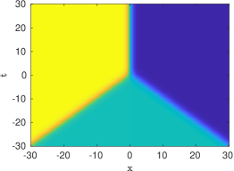
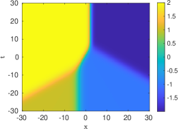
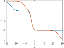
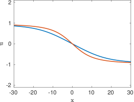
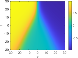
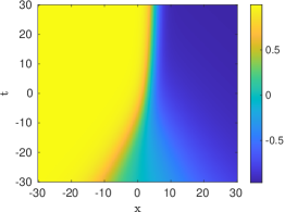
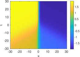
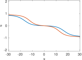
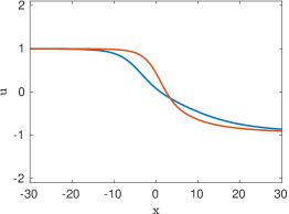
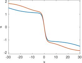
In the following, we analyze several special cases of measures . Illustrations of the corresponding entire solutions can be found in Figure 1. The simplest possible example of a bounded entire solution corresponds to being a Dirac mass located at some point . In that case we clearly have for all . A more interesting situation is obtained when for some . A direct calculation then shows that , where is the viscous shock profile given by
| (5.14) |
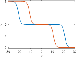
As soon as contains more than two Dirac masses, the solution given by (5.4) describes the merger of several viscous shocks into a single one. A typical example is for which
| (5.15) |
It is clear that as , whereas for large negative times a direct calculation shows that with . Thus the solution (5.15) realizes the merger of a pair of traveling viscous shocks into a single steady shock. Mergers of more than two shocks can be described in a similar fashion.
We next consider examples where the measure has an absolutely continuous component. In analogy to finitely many Dirac masses describing discrete superpositions of shocks and subsequent mergers, a continuous measure can be thought of as representing a continuous superposition of shocks with continuous merger events. Such an interpretation is reminiscent of Hamel and Nadirashvili’s characterization of entire solutions to the Fisher-KPP equation in , see [10].
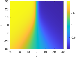
The prototypical example of an absolutely continuous measure is the Lebesgue measure on the interval , which was considered in [16, 17]. In that case, the entire solution (5.10) of the heat equation takes the simple form
| (5.16) |
so that . When , we obtain after integrating by parts
so that the entire solution (5.6) of Burgers’ equation has the following expression :
| (5.17) |
It remains to obtain a more explicit formula for . When a direct calculation shows that
| (5.18) |
where is the (non-normalized) error function. Using (5.17), (5.18), it is not difficult to verify that
the convergence being uniform for provided as . This is of course in full agreement with Propositions 1.2 and 1.3. For positive times, the analogue of (5.18) is
| (5.19) |
where is the Dawson function
It easily follows from (5.17) and (5.19) that as , in agreement with Proposition 4.1.
We next investigate how the solution is modified if the measure contains in addition a Dirac mass. Assume for instance that , where is again the Lebesgue measure on , and let be the entire solution of (5.1) associated with the measure . The same calculations as before show that
| (5.20) |
where is given by (5.16). As is easily verified, the asymptotic behavior as is unchanged. However, the presence of a Dirac mass at the origin can be detected by looking at the solution for large negative times. Indeed, a direct calculation reveals that, for all ,
| (5.21) |
Finally, we consider the measure , which includes a Dirac mass at , and we investigate the asymptotic behavior of the corresponding solution as . It is clear that
Using the expression (5.19) and the asymptotic behavior of the Dawson function at infinity, we find
Defining , we see that as , and we conclude that as . In other words, the presence of a Dirac mass at is responsible for a logarithmic shift in the position of the viscous shock, as discussed in Remark 4.2.
5.3 Asymptotic analysis of entire solutions as
The properties of the measure in (5.4) are reflected in the asymptotic behavior of the entire solution in the ancient limit . Some results in this direction were already stated in Propositions 1.2 and 1.3, and illustrated by the examples considered in the previous section. Our goal here is to perform a more systematic study of the ancient limit for entire solutions of (5.1). Our main results are Propositions 5.6 and 5.8 below, which immediately imply the statements given in the introduction, and also extend the results obtained in [16, Section 7].
To gain a first intuitive understanding, we consider the entire solution (5.4) in a Galilean frame moving with speed . In the spirit of Appel’s transformation (5.7), we also introduce the inverse time , so that the ancient limit becomes a standard short time limit in the new variable . A simple calculation shows that
| (5.22) |
where is the heat kernel (5.8). We investigate the behavior of (5.22) in the limit , for a fixed (for simplicity, we assume here that ). The denominator in the right-hand side of (5.22) is exactly the solution at time of the heat equation with initial data , evaluated at point . When is small, this quantity is an average of the measure in a small neighborhood of the point . The numerator has a similar interpretation, except that the initial measure is now .
These observations strongly suggest that should converge to as , whenever belongs to the support of the measure . If , we expect that the ancient limit of will depend on the behavior of the measure near the point in that is closest to . The results established below show that these heuristic considerations are indeed correct.
In what follows, we always assume that is probability measure supported in a bounded interval of , and we denote by the bounded entire solution of (5.1) given by (5.4). We first consider the case where .
Proposition 5.6.
-
Proof . By Galilean invariance, it is sufficient to prove (5.23) in the particular case where . We proceed as in the proof of Proposition 5.5. Given we observe that
(5.24) where for we denote
Assuming that and recalling that , we observe that , hence
(5.25) On the other hand, we obviously have
(5.26) where since . Taking with , we deduce from (5.25), (5.26) that converges to zero as , uniformly for . If we now return to (5.24), we conclude that
(5.27) Since was arbitrary, the left-hand side in (5.27) actually vanishes, which gives (5.23).
Remark 5.7.
The assumption that as is optimal in general. As can be seen from Example 5.4, where is the Lebesgue measure on , the conclusion (5.23) fails for any if does not converge to zero. However, if the measure has an atom at which is an isolated point in , it is easy to verify that (5.23) holds with for some .
The case where is more difficult to treat, see [16, Lemma 7.2] for an attempt in this direction. For simplicity, we formulate our result in the case where , but as already mentioned this does not restrict the generality.
Proposition 5.8.
Remark 5.9.
-
Proof . The proof of case (i) uses exactly the same arguments as in Proposition 5.6. Assume for instance that , so that is the point in that is closest to the origin. If is large, the leading contributions in the representation formula (5.4) correspond to the restriction of the measure to a small neighborhood of . More precisely, given any , we find
where and is as in (5.23). This gives (5.29) when , and the other case is treated similarly.
We now concentrate on the case (ii) where , which requires a more careful analysis because both intervals and equally contribute to the representation formula (5.4) when is large. Denoting
we easily find that converges to zero as uniformly for , provided as . So it remains to determine the behavior of for large negative times.
For this purpose we first observe that
so that where
(5.31) Using the change of variables we can write
(5.32) where are positive measures on with . If we substitute (5.32) in (5.31) we obtain the nicer expression
(5.33) Summarizing the results obtained so far, we have shown that, given any ,
(5.34) where is the viscous shock (5.14) connecting the states and . The bound (5.34) holds provided as .
To go further, we need properties of the shift function that are established in Section A.4.
Lemma 5.10.
The shift function defined in (5.33) satisfies the uniform bounds
(5.35) Moreover is independent of the parameter in the ancient limit, in the sense that
(5.36) provided as .
In the rest of the proof, we assume without loss of generality that . For any , we denote by the unique real number satisfying
| (5.37) |
Note that by (5.35), so that the equation for has indeed a unique solution. The following properties of will also be established in Section A.4.
Lemma 5.11.
If the function defined by (5.37) satisfies
| (5.38) |
Equipped with Lemmas 5.10 and 5.11, we now conclude the proof of Proposition 5.8. For large enough and , we want to estimate the quantity
| (5.39) |
The first term in the right-hand side is controlled using (5.34). To bound the second one, we consider three different regions:
- 1)
-
2)
When , the triangle inequality implies that
so that . It follows that
because as .
-
3)
The same bound holds when , and is established by a similar argument.
Summarizing, we have shown that there exists a constant such that
| (5.40) |
If we now combine (5.34), (5.39), and (5.40), we arrive at
| (5.41) |
In fact, since , it follows from (5.38), (5.41) that
| (5.42) |
where the constant does not depend on . Thus, taking the limit in (5.42), we arrive at (5.30) with .
In view of Galilean invariance, Proposition 1.3 is simply a reformulation of case (i) in Proposition 5.8. In case (ii), the solution converges to a translate of the viscous shock if the shift function has a finite limit as , or to the constant state if . A priori it is also possible that does not converge at all, if has an oscillatory behavior, but we do not have any explicit example. In any case cannot converge to zero in , because this would contradict either (5.29) of (5.30). So we see that Propositions 5.6 and 5.8 together imply Proposition 1.2.
Remark 5.12.
It is also possible to detect the presence of atoms in the measure by using a different scaling in the ancient limit. Assume for instance that . For any , the representation formula (5.4) can be written in the form
| (5.43) |
By Lebesgue’s dominated convergence theorem, the numerator in the right-hand side vanishes in the ancient limit , whereas the denominator converges to . So, if the measure has an atom at the origin, we deduce that converges to zero in as . Now, assume on the contrary that near the origin, where the density is continuous and satisfies . Using the change of variable , we can transform (5.43) into
| (5.44) |
Applying Lebesgue’s theorem again, we see that converges to in as . This explains the observations made in (5.21).
6 Long-time the asymptotics beyond shocks
Equipped with the representation formula (5.4), we now return to the discussion of -limit sets, focusing our attention to the particular case of Burgers’ equation. If , we know from Proposition 3.3 that is bounded and fully invariant under the evolution semigroup defined by (5.1). This implies that any is the evaluation at time of some bounded entire solution of (5.1). Applying Proposition 5.1, we thus find:
Corollary 6.1.
For any , where is the -limit set (1.3) corresponding to Burgers’ equation, there exists a unique probability measure on such that
| (6.1) |
This result means that, at least for Burgers’ equation, the -limit set of any solution of (5.1) with values in some interval can be identified with a subset of all probability measures supported on that interval. This does not imply, however, that any probability measure on can be realized in this way. To make the discussion more precise, let us denote
| (6.2) |
where is the translation operator and is given by (5.14). In other words is the collection of all translates of all viscous shocks, including the constants. Any corresponds, via (5.4), to a probability measure that is a convex combination of at most two Dirac masses.
We know from Proposition 4.1 that whenever is monotonically decreasing. On the other hand, Oleinik’s inequality (2.2) indicates that all solutions of (5.1) are “eventually decreasing” when . Combining these observations, it is rather tempting to conjecture that for any . Our last result provides an example that contradicts this hasty conclusion. To make a precise statement we introduce for any the function defined by
| (6.3) |
Note that is just the evaluation at time of the two-shock solution (5.15).
Proposition 6.2.
There exist initial data for Burgers’ equation such that
| (6.4) |
where is the -limit set (1.2). In particular .
In other words, Proposition 6.2 gives an example of bounded initial data such that even the “small” -limit set contains the two-shock solution (5.15), in addition to a continuum of steady shocks. More generally we conjecture that, for any probability measure on the interval , there exist initial data satisfying (2.1) such that the -limit set contains the function defined by (6.1). We believe that this (nontrivial) extension of Proposition 6.2 can be obtained following the same lines of thought as in Section 6.1 below. This question is left for future work.
Examples of -limit sets with complicated structure were also constructed for reaction-diffusion equations on the real line, see e.g. [5, 21, 22]. In those examples, nonstationary solutions appear in the -limit set as a result of a coarsening dynamics. The same idea is exploited here in our proof of Proposition 6.2, but the result is in some sense more surprising because it is not clear a priori if something like a coarsening dynamics is compatible with the constraints imposed by Oleinik’s inequality (2.2).
Remark 6.3.
In the spirit of the work of Slijepčević and the first author, one may ask if, for general initial data (including those considered in Proposition 6.2), the solution approaches locally uniformly the set at least for “almost all times”, in the precise sense considered in [9]. We hope to address that interesting question in a near future.
6.1 Shock mergers in the -limit set
In this section, we construct bounded initial data for Burgers’ equation (5.1) such that the corresponding solution exhibits mergers of viscous shocks at the origin for an infinite sequence of times. The construction is based on the Cole-Hopf representation formula (5.6).
Definition 6.4.
For any , let be the solution of the linear heat equation with initial data
| (6.5) |
Since is an exact solution of the heat equation, the parabolic maximum principle implies that for all and all . The following two lemmas give more precise estimates on the function and its derivative.
Lemma 6.5.
For any and any the following estimates hold :
| (6.6) |
Estimates (6.6) provide a good approximation of the solution for large times. The short time behavior near the origin is described by the following result.
Lemma 6.6.
Assume that and . Then
| (6.8) |
-
Proof . Let . Then is again a solution of the heat equation, hence
(6.9) Our main goal is to find an upper bound on in the region region where . We observe that where
(6.10) where denotes the complementary error function. In the last equalities in (6.10), we used the changes of variables to reduce the integrals to an error function. By assumption, we have , and it is known that is a decreasing function on which satisfies for all . This leads to the upper bound
which proves the first part of (6.8). The second inequality is established by a similar calculation based on the identity
This concludes the proof of Lemma 6.6.
We now explain our strategy to prove Proposition 6.2. If is large enough, the solution of Burgers’ equation given by satisfies, by Lemma 6.6,
whereas when by Lemma 6.5. In other words describes, for relatively small times, the merger of a pair of viscous shocks at the origin, but in the long time regime actually converges to zero, uniformly in on compact intervals. The idea is to construct, by superposition, a solution of (5.1) which exhibits infinitely many such mergers, along an appropriate sequence of times.
Proof of Proposition 6.2 (first part). Fix and let be a sequence of times such that
| (6.11) |
We consider the function defined by
| (6.12) |
where is given by Definition 6.4 with . Since , it is clear that the series in (6.12) converge uniformly on compact sets in space-time, and that is a solution of the heat equation on . We are interested in the corresponding solution of Burgers’ equation, given by
| (6.13) |
As for all , we have for all by the maximum principle, and it follows that , so that is a bounded solution of Burgers’ equation. We shall show that, for any sufficiently large , this solution exhibits a merger of viscous shocks at the origin on the time interval . More precisely, we shall prove that
| (6.14) |
To establish (6.14), we fix a large , and we assume that ] and . If , we know from Lemma 6.6 that
| (6.15) |
because since . In view of (6.11), estimate (6.15) shows that, in the space-time region under consideration, all terms with can be neglected in the sum (6.12) defining , namely
If , we apply Lemma 6.5 and obtain the bound
| (6.16) |
where the left-hand side is strictly positive since . Again it follows from (6.11), (6.16) that the terms with can be neglected in the sum (6.12), in the sense that
Summarizing, we have shown that the function defined by (6.12) satisfies when ] and , where
| (6.17) |
More precisely we have
| (6.18) |
where the estimate for the derivative is obtained in the same way using Lemmas 6.5 and 6.6. We now take , so that both terms in the right-hand side of (6.17) are of comparable size. With that choice, we have , and using estimates (6.18) we easily deduce that the function indeed satisfies (6.14).
So far we have shown that the function introduced in (6.3) belongs to the -limit set when . But the argument above also implies that, given any ,
which shows that the -limit set contains the entire two-shock solution (5.15) (as is clear from time invariance). So we conclude that , as asserted in (6.4).
6.2 Repair along the family of steady shocks
In the topology of , the two-shock solution (5.15) converges to zero as and to the steady shock as . Such a heteroclinic connection is obviously not chain recurrent in the sense of Proposition 3.2. As a consequence, for the initial data constructed in the previous section, the -limit set must be larger than the heteroclinic orbit given by the two-shock solution. In this section, we show that contains in addition a continuum of steady shocks, as stated in Proposition 6.2.
To prove the claim, we need to control the function introduced in Definition 6.4 for some intermediate times that are not covered by Lemmas 6.5 and 6.6.
Lemma 6.7.
For any fixed we have, as ,
| (6.19) |
where convergence is uniform in for any . A similar asymptotic expansion also holds for the spatial derivative .
-
Proof . To establish (6.19) it is convenient to use an explicit expression for the function . Starting from the definition
and proceeding as in (6.10), we obtain the tractable formula
(6.20) where
(6.21) In what follows, we assume that for some fixed , and we consider the limit for in some fixed interval . Using the asymptotic expansion of the complementary error function
we easily find that
(6.22) Next, observing that as because , we see that the second term in the expression (6.21) of is negligible compared to the first one. Since
we thus find
(6.23) Finally, replacing (6.22) and (6.23) into (6.20), we arrive at (6.19). A corresponding asymptotic expansion for the derivative is obtained in the same way.
Proof of Proposition 6.2 (second part). We consider again the solution of the heat equation given by (6.12), and we evaluate it along the sequence of times , for some fixed . The main contribution to the sum comes from the term where , and using Lemma 6.7 with we obtain
| (6.24) |
where convergence holds uniformly for . The terms where can be easily estimated using the trivial bound , leading to
| (6.25) |
where the right-hand side is much smaller than (6.24) since . Finally, for the terms where , we use the simple bound which gives
| (6.26) |
Again, for , the right-hand side is much smaller than (6.24) because the sequence grows fast enough as and .
Summarizing, it follows from (6.24), (6.25), (6.26) that the function defined by (6.12) satisfies
uniformly for , and a similar expansion also holds for the first derivative . So, we deduce that the solution of Burgers’ equation defined by (6.12), (6.13) satisfies, for any ,
This implies that the -limit set contains the viscous shock for any value of , hence for any since is closed in . The proof of (6.4) is now complete.
7 Discussion
We presented results on long-time behavior in scalar conservation laws on the real line, both in the case of a general convex flux and in the special case of Burgers’ equation with quadratic flux. Our main results include a general definition and characterization of -limit sets, the convergence to single shocks for monotone data, and the construction of initial data for which the -limit set does not consist of a constant state nor of the translates of a single shock. The latter result was established in the context of Burgers’ equation, where a somewhat explicit representation of all entire solutions in terms of compactly supported probability measures is available. Since all elements in the -limit set are entire solutions, this characterization provides a ”list” of candidates for elements in the -limit set.
We mentioned throughout several open problems and conjectured some answers. We revisit some of those here in a broader context and point to some other potentially interesting questions.
As a first step towards a complete characterization, one can ask what functions may be found within an -limit set. Candidates are entire solutions, which, in the case of Burgers’ equation, are described somewhat explicitly through a one-to-one correspondence with compactly supported probability measures on the real line. Even beyond the goal of describing the long-time behavior of general solutions, it would be quite interesting to characterize entire solutions of scalar conservation laws with convex, not necessarily quadratic flux. In the absence of a direct connection with the heat equation, we think that a description of bounded solutions in terms of their ancient limits in suitably rescaled variables might provide an avenue for progress in this direction. Note that solutions representing the superposition of two viscous shocks as can be constructed under generic assumptions on the flux function, see [28].
On the other hand, it would be interesting to extend the analysis of ancient solutions and possibly the characterization of -limit sets to the complex-valued Burgers’ equation, where the Cole-Hopf transformation is still at hand, but upper bounds, Oleinik’s inequality, and the positivity that is essential in the characterization of ancient solutions are not available; see [23] for results on blowup in this context.
Given the characterization of entire solutions in Burgers’ equation, we conjectured in Section 6 that any entire solution of that equation can be found in the -limit set for appropriate initial data. Beyond Burgers’ equation, one may find it plausible that the existence of shock mergers in specific -limit sets can be established, by controlling the interaction of shocks and rarefaction waves without the conjugation to a linear heat equation and the associated superposition principle.
A more ambitious result would characterize the entire -limit set. We showed that for monotone initial data, one only finds a single shock (together with its translates) or a family of constant states. We conjectured that in the example considered in Proposition 6.2, the -limit set actually consists of the shock merger itself and of the family of steady shocks with smaller amplitude, which together form a chain recurrent set. Given the ancient asymptotics of entire solutions, all nonconstant elements of the -limit sets can be thought of as continuous or discrete superpositions of shocks and their eventual merger into a single shock. The natural question in this direction is whether different shock mergers can occur within a single -limit set. Eventually, one may hope to determine which subsets of the set of ancient solutions may occur as -limit sets, that is, to decide if any additional restrictions beyond compactness, connectedness, and chain recurrence are imposed by the dynamics.
Clearly, all of the questions above can be asked for and for , that is in a fixed frame of reference or up to translations. Our introduction of , while seemingly natural, can of course be questioned. One could ask for a more narrow characterization, limiting the allowed translations for instance to almost Galilean shifts as suggested in Remark 3.5. To clarify the role of the shifts, it would be interesting to identify -limit sets that actually depend on the class of allowed spatial translates. More specifically, one can ask if for all , the set defined by (1.3) coincides with the -limit set obtained by restricting the class of allowed shifts to almost Galilean ones.
Beyond the structure of -limit sets, one can investigate the dynamics for large but finite times. While Burgers’ equation is not a gradient flow, our results basically show that the long-term asymptotics of solutions are to a large extent determined by equilibria, up to Galilean boosts. While we did show that solutions other than equilibria, particularly shock mergers, can occur in the -limit set, it is conceivable to conjecture that those occur only ”rarely” in time, a statement that one could attempt to quantify in the spirit of the work of S. Slijepčević and the first author [9]; see Remark 6.3.
Finally, a number of subtle questions arise when attempting to characterize the set of initial data that lead to a specific -limit set. From local stability of viscous shocks, one can conclude that the basin of attraction is open (in appropriate topologies). On the other hand, we showed that the basin contains all monotone initial data with the same limits at . The construction of repeating shock mergers suggests robustness of this asymptotic behavior at least in a spatially uniform topology. We note however that such questions on the basin of attraction of an -limit set do not appear to have been answered in the case of mergers between layers in the Allen-Cahn equation [5, 21, 22]. Despite the apparent similarities between the results there and our construction, it is worth noticing that in our case, all equilibria and traveling waves are asymptotically stable, whereas the Allen-Cahn equation accommodates a large family of unstable equilibria and traveling waves, including the zero solution, spatially periodic equilibria, and traveling waves connecting those equilibria to stable solutions; see for instance [26]. We are not aware of results that connect the role of these unstable equilibria to the description of long-term dynamics through -limit sets as attempted here and in [5, 21, 22].
Appendix A Appendix
A.1 Oleinik’s inequality
If is a solution of (1.1) with initial data satisfying (2.1), we define
| (A.1) |
where is defined in (2.2). The function is smooth, and it is clear by construction that for all whenever is sufficiently small. Indeed, since solves equation (1.1) with bounded initial data, we know that there exist positive constants and such that when . Now a direct calculation shows that solves the equation
| (A.2) |
where in the second line we used the fact that for all . By the maximum principle, the differential inequality (A.2) implies that stays negative for all times , which gives inequality (2.2).
A.2 Proof of Lemma 3.1
We prove here that the solution of of (1.1) depends continuously on the initial data in the topology of . Our starting point is the integral equation associated with (1.1), namely
| (A.3) |
where is the heat kernel (5.8) and denotes convolution in space. Straightforward calculations show that there exists a constant such that
| (A.4) |
for all and all . To prove the desired continuity property, we fix and consider two sets of initial data such that . Denoting , , and using (A.4), we can estimate
where . The quantity thus satisfies an integral inequality that can be solved using a variant of Grönwall’s lemma, see [12, Lemma 7.1.1]. This gives an estimate of the form , for some universal constants , which shows that the solution of (A.3) depends continuously on the initial data in the topology of , uniformly in time on compact intervals.
A.3 Proof of the – estimate (4.16)
Assume that is a smooth convex function such that and for all . If is a solution of (4.15) with initial data , we compute
| (A.5) |
where we used the crucial observation that , because is convex and is decreasing. As a first application, we take , where is a small parameter. Using (A.5) we easily obtain , for any . Then, invoking Lebesgue’s monotone convergence theorem, we can take the limit and arrive at
| (A.6) |
In a second step, we choose in (A.5) and we use the celebrated Nash inequality
| (A.7) |
see [3]. Taking (A.6) into account and assuming , we obtain the differential inequality
which can be integrated to give the – estimate
| (A.8) |
where .
Finally, to estimate the norm of , we can either bound the norm for all integers , or use a duality argument, see [6]. We follow here the latter approach and consider the dual equation
| (A.9) |
which has similar properties as (4.15). In particular, proceeding as in (A.5), we find
| (A.10) |
because by convexity. We deduce that estimates (A.6), (A.8) also hold for the solutions of (A.9). Now, if solves (4.15) with initial data and solves (A.9) with initial data , then for any the quantity is independent of , as can be easily verified by differentiation. It follows that
| (A.11) |
where the last inequality follows from (A.8). Clearly (A.11) is equivalent to the – estimate
| (A.12) |
and the – bound in (4.16) follows immediately by combining (A.8), (A.12).
A.4 Proof of Lemmas 5.10 and 5.11
Proof of Lemma 5.10..
Since are positive measures supported on the interval , it is clear that the functions introduced in (5.32) satisfy the estimates
which immediately imply (5.35) in view of the definition (5.33) of . On the other hand, if , we have the identity
| (A.13) |
and proceeding as in the proof of Proposition 5.6 we easily obtain, if ,
where . If as , it follows that
which together with (A.13) implies the desired estimate (5.36). ∎
Proof of Lemma 5.11..
Let us define . For any , we observe that
| (A.14) |
Indeed, if , we have
The middle term in the right-hand side can be estimated with the help of (5.35) :
where we used the fact that . The other terms are controlled by (5.36), which gives
and taking the limit we obtain the first part of (A.14). The second claim follows by an elementary argument.
We now return to the shift function defined by (5.37). We have by (5.35)
so that
In view of (A.14), it follows in particular that as , which is the first claim in (5.38). Moreover, if , we have
Since as , the last term in the right-hand side converges to zero by (5.36). We deduce that too, which concludes the proof of (5.38). ∎
References
- [1]
- [2] P. Appell, Sur l’équation et la Théorie de la chaleur (French). J. Math. Pures Appl. 8 (1892), 187–216.
- [3] E. Carlen and M. Loss, Sharp constant in Nash’s inequality. Int. Math. Res. Not. 1993 (1993), 213–215.
- [4] J. D. Cole, On a quasi-linear parabolic equation occurring in aerodynamics. Quart. Appl. Math. 9 (1951), 225–236.
- [5] J.-P. Eckmann and J. Rougemont, Coarsening by Ginzburg-Landau dynamics. Commun. Math. Phys. 199 (1998), 441–470.
- [6] E. B. Fabes and D. W. Stroock, A new proof of Moser’s parabolic Harnack inequality using the old ideas of Nash. Arch. Rational Mech. Anal. 96 (1986), 327–338.
- [7] J. E. Franke and J. F. Selgrade, Abstract -limit sets, chain recurrent sets, and basic sets for flows. Proc. Amer. Math. Soc. 60 (1976), 309–316.
- [8] H. Freistühler and D. Serre, stability of shock waves in scalar viscous conservation laws. Commun. Pure Appl. Math. 51 (1998), 291–301.
- [9] Th. Gallay and S. Slijepčević, Distribution of energy and convergence to equilibria in extended dissipative systems. J. Dynam. Differential Equ. 27 (2015), 653–682.
- [10] F. Hamel and N. Nadirashvili, Travelling fronts and entire solutions of the Fisher-KPP equation in . Arch. Ration. Mech. Anal. 157 (2001), 91–163.
- [11] G. M. Henkin, Asymptotic structure for solutions of the Cauchy problem for Burgers type equations. J. Fixed Point Theory Appl. 1 (2007), 239–291.
- [12] D. Henry, Geometric Theory of Semilinear Parabolic Equations. Lectures Notes in Mathematics 840, Springer, 1981.
- [13] G. M. Henkin, A. A. Shananin, and A. E. Tumanov, Estimates for solutions of Burgers type equations and some applications. J. Math. Pures Appl. 84 (2005), 717–752.
- [14] E. Hopf, The partial differential equation . Commun. Pure Appl. Math. 3 (1950), 201–230.
- [15] A. M. Il’in and O. A. Oleinik, Asymptotic behavior of solutions of the Cauchy problem for some quasi-linear equations for large values of the time (Russian). Mat. Sb. (N.S.) 51(93) (1960), 191–216.
- [16] U. P. Karunathilake, A representation theorem for certain solutions of Burgers’ equation. PhD thesis, University of Minnesota, May 2007.
- [17] C. E. Kenig and F. Merle, A Liouville theorem for the viscous Burgers equation. J. d’Analyse Math. 87 (2002), 281–298.
- [18] A. Matsumura and K. Nishihara, Asymptotic stability of traveling waves for scalar viscous conservation laws with non-convex nonlinearity. Commun. Math. Phys. 165 (1994), 83–96.
- [19] A. Mielke and G. Schneider, Attractors for modulation equations on unbounded domains – existence and comparison. Nonlinearity 8 (1995), 743–768.
- [20] K. Nishihara and Huijiang Zhao, Convergence rates to viscous shock profile for general scalar viscous conservation laws with large initial disturbance. J. Math. Soc. Japan 54 (2002), 447–466.
- [21] P. Poláčik, Examples of bounded solutions with nonstationary limit profiles for semilinear heat equations on . J. Evol. Equ. 15 (2015), 281–307.
- [22] P. Poláčik, Threshold behavior and non-quasiconvergent solutions with localized initial data for bistable reaction-diffusion equations. J. Dynam. Differential Equ. 28 (2016), 605–625.
- [23] P. Poláčik and V. Šverák, Zeros of complex caloric functions and singularities of complex viscous Burgers’ equation. J. Reine Angew. Math. 616 (2008), 205–217.
- [24] M. H. Protter and H. F. Weinberger, Maximum principles in differential equations. Prentice-Hall, Englewood Cliffs, 1967.
- [25] W. Rudin, Real and complex analysis. McGraw-Hill, 1966.
- [26] A. Scheel, Coarsening fronts. Arch. Rational Mech. Anal. 181 (2006), 505–534.
- [27] D. Serre, Systèmes de lois de conservation. I: Hyperbolicité, entropies, ondes de choc (French). Diderot, Paris, 1996.
- [28] D. Serre, Solutions globales () des systèmes paraboliques de lois de conservation (French). Annales de l’Institut Fourier 48 (1998), 1069–1091.
- [29] D. Serre, -stability of nonlinear waves in scalar conservation laws. In: Handbook of Differential Equations, Evolutionary Equations Vol. I, 473–553, C. M. Dafermos and E. Feireisl (eds), Elsevier/North-Holland, 2004.
- [30] D. V. Widder, Positive temperatures on an infinite rod. Trans. Amer. Math. Soc. 55 (1944), 85–95.
- [31] D. V. Widder, The Role of the Appell Transformation in the Theory of Heat Conduction. Trans. Amer. Math. Soc. 109 (1963), 121–134.
Thierry Gallay
Institut Fourier, Université Grenoble Alpes, 100 rue des Maths, 38610 Gières,
France
Email : Thierry.Gallay@univ-grenoble-alpes.fr
Arnd Scheel
School of Mathematics, University of Minnesota
127 Vincent Hall, 206 Church St. SE, Minneapolis, MN 55455, USA
Email : scheel@math.umn.edu