Visual illusions via neural dynamics: Wilson-Cowan-type models and the efficient representation principle
Abstract
We reproduce supra-threshold perception phenomena, specifically visual illusions, by Wilson-Cowan-type models of neuronal dynamics. Our findings show that the ability to replicate the illusions considered is related to how well the neural activity equations comply with the efficient representation principle. Our first contribution consists in showing that the Wilson-Cowan (WC) equations can reproduce a number of brightness and orientation-dependent illusions. Then, we formally prove that there can’t be an energy functional that the Wilson-Cowan dynamics are minimizing. This leads us to consider an alternative, variational modelling which has been previously employed for local histogram equalization (LHE) tasks. In order to adapt our model to the architecture of V1, we perform an extension that has an explicit dependence on local image orientation. Finally, we report several numerical experiments showing that LHE provides a better reproduction of visual illusions than the original WC formulation and that its cortical extension is capable to reproduce also complex orientation-dependent illusions.
New & Noteworthy: We show that the Wilson-Cowan equations can reproduce a number of brightness and orientation-dependent illusions. Then, we formally prove that there can’t be an energy functional that the Wilson-Cowan equations are minimizing, making them sub-optimal with respect to the efficient representation principle. We thus propose a slight modification that is consistent with such principle and show that this provides a better reproduction of visual illusions than the original Wilson-Cowan formulation. We also consider the cortical extension of both models in order to deal with more complex orientation-dependent illusions.
1 Introduction
The goal of this work is to point out the intimate connections existing between three popular approaches in vision science: the Wilson-Cowan equations, the study of visual brightness illusions, and the efficient representation theory.
As other articles in this special issue make abundantly clear, Wilson-Cowan equations have a long and successful story of modelling cortical low-level dynamics [Cowan et al., 2016]. Nonetheless, the study of psychophysics by Wilson-Cowan equations ([Adini et al., 1997, Herzog et al., 2003, Bertalmío and Cowan, 2009, Ernst et al., 2016, Bertalmío et al., 2017, Wilson, 2003, Wilson, 2007, Wilson, 2017]) is a topic that hasn’t been addressed much in neuroscience, and we are not aware of publications in which Wilson-Cowan equations are used for predicting brightness illusions. In this work, we aim to fill this gap.
The study of visual illusions has always been key in the vision science community, as the mismatches between reality and perception provide insights that can be very useful to develop new models of visual perception [Kingdom, 2011] or of neural activity [Eagleman, 1959, Murray and Herrmann, 2013], and also to validate the existing ones. It is commonly accepted that visual illusions arise due to neurobiological constraints [Purves et al., 2008] that modify the underpinned mechanisms of the visual system.
The efficient representation principle, introduced by Attneave [Attneave, 1954] and Barlow [Barlow et al., 1961], states that neural responses aim to overcome these neurobiological constraints and to optimize the limited biological resources by being tailored to the statistics of the images that the individual typically encounters, so that visual information can be encoded in the most efficient way. This principle is a general strategy observed across mammalian, amphibian and insect species [Smirnakis et al., 1997] and is embodied by neural processing according to abundant experimental evidence [Fairhall et al., 2001, Mante et al., 2005, Benucci et al., 2013].
Our work aims at pulling together the three approaches just mentioned, providing a more unified framework to understand vision mechanisms. First, we show that the Wilson-Cowan equations are able to qualitatively reproduce a number of visual illusions. Secondly, we formally prove that Wilson-Cowan equations (with constant input) are not variational, in the sense that they are not minimizing any energy functional. Next, we detail how a simple modification turning the Wilson-Cowan equations variational yields a local histogram equalisation method that is consistent with the efficient representation principle. We finally show how this new formulation provides a better reproduction of visual illusions than the Wilson-Cowan model.
We remark that our model has to be intended as a proof of concept, whose objective is the reproduction of perceptual phenomena at a macroscopic level with no quantitative assessment on analogous psychophysical data. There are in fact very important limitations for doing that, since such comparison would require both a perfect knowledge of how behavioural data were collected, and a tuning of the model parameters to match with the observed perception. Nonetheless, we believe that the numerical evidence of our experiments and our theoretical considerations can be used for future research studies comparing our computational results with the ones corresponding to experiments coming from psychophysics.
2 Materials and methods
2.1 Visual illusions
Computational models able to reproduce visual illusions represent very effective methods to test new hypotheses and generate new insights, both for neuroscience and applied disciplines such as image processing. Illusions can be classified according to the main feature detection mechanisms involved during the visual process [Shapiro and Todorovic, 2016]. In this contribution we considered two main groups of visual illusions to assess the efficacy of our model in reconstructing the perceptual process: brightness illusions and orientation-dependent illusions.
2.1.1 Brightness illusions
Brightness illusions are a class of phenomena where image regions with the same gray level are perceived as having different brightness, depending on the shapes, arrangement and gray level of the surrounding elements. Fig. 1 shows the nine brightness illusions we have chosen to perform tests on in this paper. They are all very popular and at the same time they represent a diverse set, as we can see from the following descriptions.
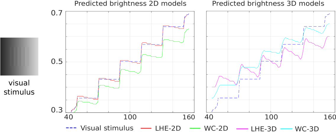
White’s illusion:
the left gray rectangle appears darker than the right one, while both are identical [White, 1979] (Fig. 1(a)).
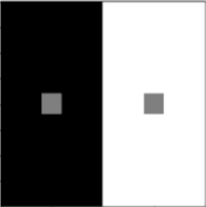
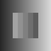
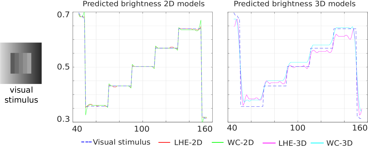
Simultaneous brightness contrast:
the left gray square appears lighter than the right one, while both are identical [Brucke, 1865] (Fig. 1(b)).
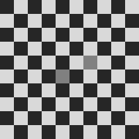
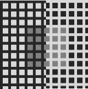
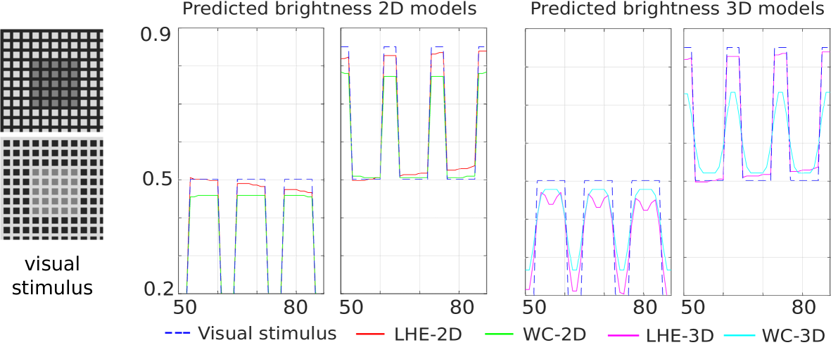
Checkerboard illusion:
the mid-gray square in the fifth column appears darker than the one in the seventh column, while both are identical [DeValois and DeValois, 1990] (Fig. 1(c)).
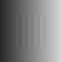
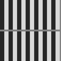
Chevreul illusion:
a pattern of homogeneous bands of increasing intensity from left to right is presented. However, the bands in the image are perceived as inhomogeneous, i.e. darker and brighter lines appear at the borders between adjacent bands [Ratliff, 1965] (Fig. 1(d)).
Chevreul cancellation:
when the order of the bands is reversed, now decreasing in intensity from left to right, the effect is cancelled [Geier and Hudák, 2011] (Fig. 1(e)).
Dungeon illusion:
two gray rectangles are perceived as darker or lighter depending on the gray intensities of both the background and the grid, see [Bressan, 2001]. The left rectangle is perceived as darker than the one on the right (Fig. 1(f)).
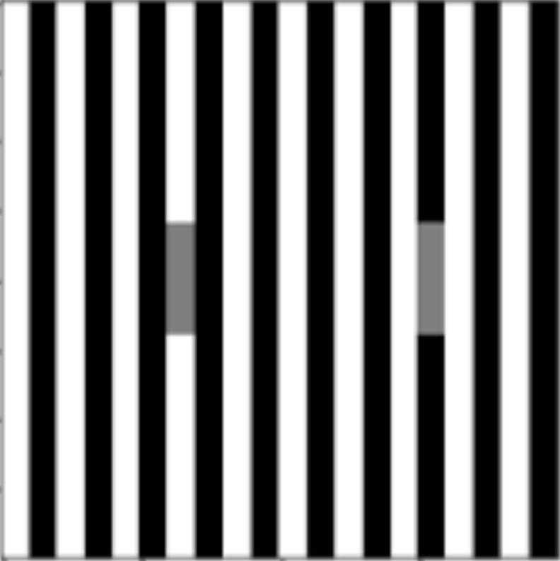
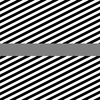
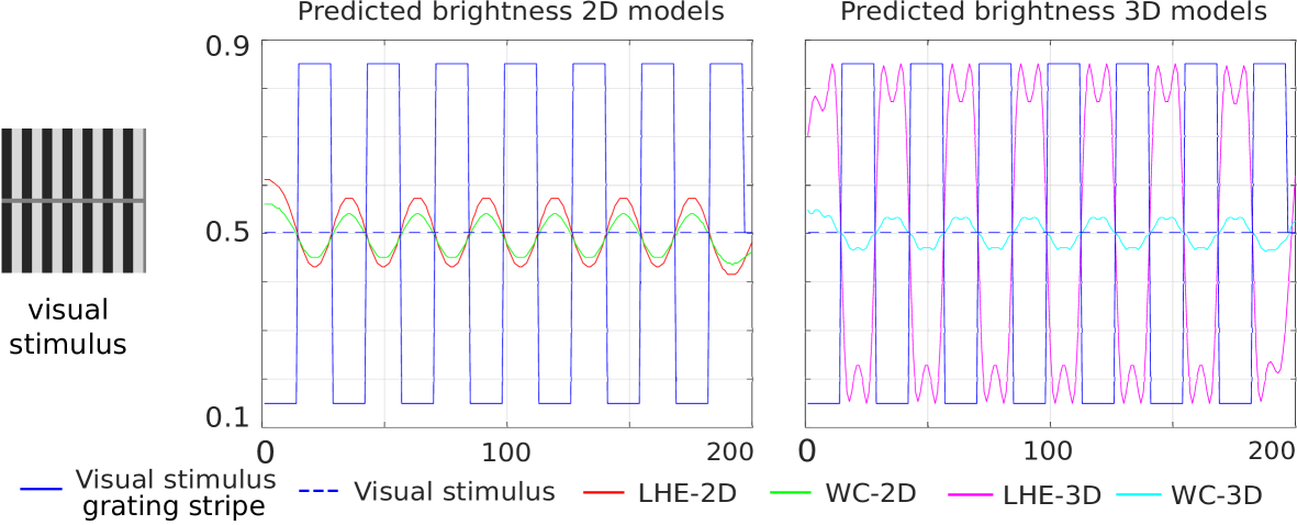
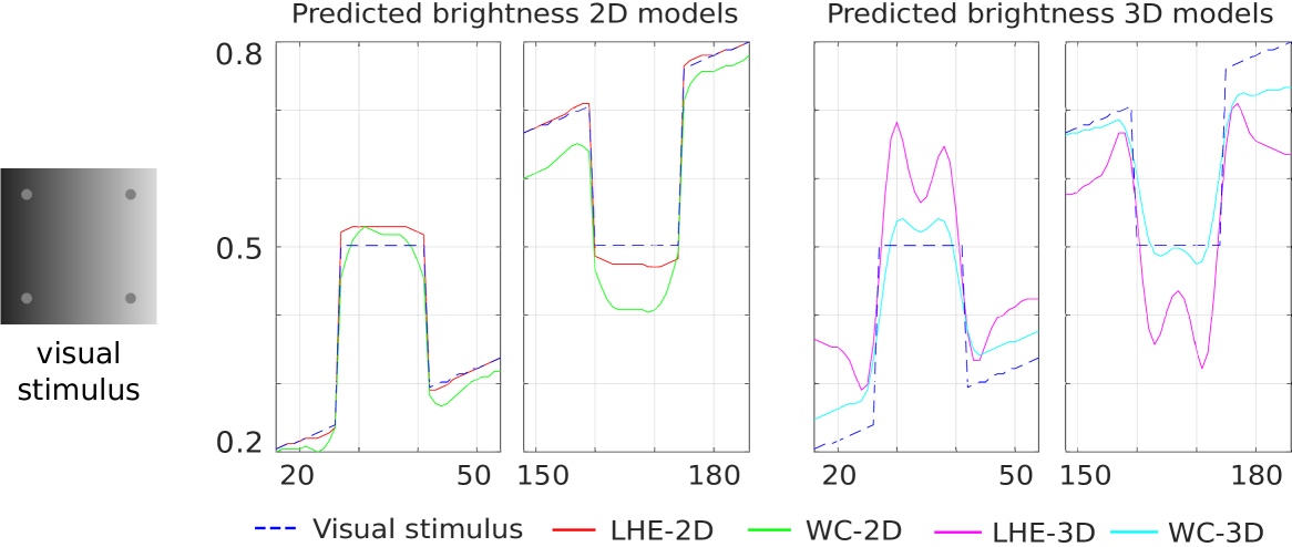
Grating induction:
the background grating (which can be tuned to different orientations) induces the appearance of a counter-phase grating in the homogeneous gray horizontal bar [McCourt, 1982] (Fig. 1(g)).
Hong-Shevell illusion:
the mid-gray half-ring on the left appears darker than the one on the right, while both are identical [Hong and Shevell, 2004] (Fig. 1(h)).
Luminance illusion:
four identical dots over a background where intensity increases from left to right, and the dots on the left are perceived being lighter than the ones on the right [Kitaoka, 2006] (Fig. 1(i)).

2.1.2 Orientation-dependent illusions
We also consider orientation-dependent illusions, where the perceptual phenomenon (e.g. in terms of brightness or contrast) is affected by the orientation of the image elements.
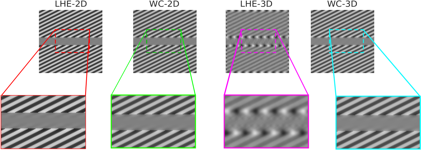
Poggendorff illusion.
The Poggendorff illusion, presented in the modified version considered in this work in Fig. 2(a), is a very well known geometrical optical illusion in which the presence of a central surface induces a misalignment of the background lines. This illusion depends both on the orientation of the background lines and the width of the central surface [Weintraub and Krantz, 1971], as the more the angle is close to the less is the bias, but in this example the perceived bias is also dependent on the brightness contrast between central surface and background lines.
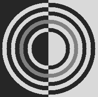
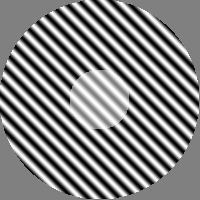
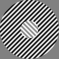
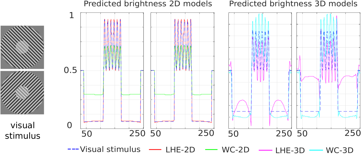
Tilt illusion.
The Tilt illusion is a phenomenon where the perceived orientation of a test line or grating is altered by the presence of surrounding lines or a grating with a different orientation. In our case we consider the effect that the orientation of a surround grating pattern has on the perceived contrast of a grating pattern in the center: the inner circles in Figs. 2(b) and 2(c) are identical but the latter is perceived as having more contrast than the former.
2.2 Wilson-Cowan-type models for contrast perception
In this section we introduce four different evolution equations derived from the Wilson-Cowan formulation, that will be studied in this paper. We recall that, denoting by the state of a population of neurons with spatial coordinates at time , the Wilson-Cowan equations proposed in [Wilson and Cowan, 1972, Wilson and Cowan, 1973] can be written111In [Wilson and Cowan, 1972] the sigmoid function is applied outside of the integral term and not only on the activity as in (2.1). This corresponds to an “activity-based” model of neuron activation, while (2.1) corresponds to a “voltage-based” one. See [Faugeras, 2009], where the two models are shown to be equivalent. as
| (2.1) |
where and are fixed parameters, is a non-linear sigmoid saturation function, the kernel models interactions at two different spatial locations and (we will assume that the integral of is normalised to ) and is the input signal.
2.2.1 Wilson-Cowan equations do not fulfill any variational principle
Over the last thirty years, the use of variational methods in imaging has become increasingly popular as a regularisation strategy for solving general ill-posed imaging problems in the form
| (2.2) |
Here, represents a given degraded image and a (possibly non-linear) operator describing the degradation (e.g. noise, blur, under-sampling, etc.)
Due to the lack of fundamental properties such as existence, uniqueness and stability of the solution of the problem (2.2), the idea of regularisation consists of incorporating a priori information on the desired image and on its closeness to the data by means of suitable variational terms. This gives rise, in particular, to variational methods where one looks for an approximation of the real solution by solving
| (2.3) |
where is the energy functional combining regularisation and data fit, depending also on the given image . A popular way to solve the variational problem consists in finding as the steady-state solution of the evolution equation given by the gradient descent of the energy functional
| (2.4) |
under appropriate conditions on the boundary of the image domain.
In the context of vision science, evolution equations have been originally used as a tool to describe the physical transmission, diffusion and interaction phenomena of stimuli in the visual cortex [Beurle and Matthews, 1956, Wilson and Cowan, 1972, Wilson and Cowan, 1973]. Variational methods are the main tool of ecological approaches, that pose the efficient coding problem [Olshausen and Field, 2000] as an optimisation problem to be solved with evolution equations that minimise an energy functional [Atick, 1992] involving natural image statistics and biological constraints. The resulting solution is optimal because it has minimal redundancy.
However, we must remark that, while considering the gradient descent of an energy functional gives always an evolution equation, the reverse is not true: not every evolution equation is minimising an energy functional. In fact, this is the case for the Wilson-Cowan equations, which do not fulfil any variational principle, as we prove in Appendix A. As a consequence, they are sub-optimal in reducing the redundancy.
We remark that it is possible to define an energy that decreases along trajectories of (2.1), as done in [French, 2004]. This ensures in particular that even though the evolution is not variational, its steady states (i.e., solutions of (2.1) that are constant in time) can indeed be obtained as critical points of this energy.
2.2.2 A modification of the Wilson-Cowan equations complying with efficient representation
Remarkably, the efficient representation principle has correctly predicted a number of neural processing aspects and phenomena like the photoreceptor response performing histogram equalisation, the dominant features of the receptive fields of retinal ganglion cells (lateral inhibition, the switch from bandpass to lowpass filtering when the illumination decreases, and, remarkably, colour opponency, with photoreceptor signals being highly correlated but color opponent signals having quite low correlation), or the receptive fields of cortical cells having a Gabor function form [Atick, 1992, Daugman, 1985, Olshausen and Field, 2000]. Efficient representation is the only framework able to predict the functional properties of neurons from a simple principle, and given how simple the assumptions are it’s really surprising that this approach works so well [Meister and Berry, 1999].
In [Bertalmío and Cowan, 2009] it is shown how a slight modification of the Wilson-Cowan formulation leads to a variational model, as we now present. Assuming that the activity signal is in the range , we can re-write equation (2.1) in terms of a sigmoid shifted by (which we take as the average signal value) and inverted in sign, thus getting:
| (2.5) |
Note that this is just a re-writing of equation (2.1), so it is still not associated to any variational method. However, if we now assume to be odd and replace the term by , we obtain
| (2.6) |
and this equation is now a gradient descent equation, as it does fulfil a variational principle.
Furthermore, under the proper choice of parameters and input signal , this evolution equation performs local histogram equalisation (LHE) [Bertalmío et al., 2007]. This is key for our purposes, since, as Atick points out [Atick, 1992], one of the main types of redundancy or inefficiency in an information system like the visual system happens when some neural response levels are used more frequently than others, and for this type of redundancy the optimal code is the one that performs histogram equalisation.
2.2.3 Accounting for orientation
Models (2.1) and (2.6) ignore orientation and as such they are not well-suited to explain a number of visual phenomena. For this reason, following [Bertalmío et al., 2019a], we extend them to a third dimension, representing local image orientation, as follows. We let be the cortical activation in V1 associated with the signal , so that encodes the response of the neuron with spatial preference and orientation preference to . Mathematically, such activation is obtained via a suitable convolution with the receptive profiles of V1 neurons, as explained in Appendix B, see also [Duits and Franken, 2010, Petitot, 2017, Prandi and Gauthier, 2017, Citti and Sarti, 2006, Sarti and Citti, 2015]. Then, denoting by the cortical response at time for any , the natural extension of equations (2.1) and (2.6) to the orientation dependent case is given by the two models:
| (2.7) | |||
| (2.8) |
where denotes the cortical activation in V1 corresponding to the visual input at spatial location and orientation preference . We remark that these models describe the dynamic behaviour of activations in the 3D space of positions and orientation. As explained in Appendix B, once a stationary solution is found, the two-dimensional perceived image can be found by simply applying the formula
| (2.9) |
2.2.4 Models under consideration
We summarise here the four models we are going to test in the following sections. The orientation-independent WC and LHE models are:
| (WC-2D) | ||||
| (LHE-2D) |
which relate to (2.1) and (2.6) by simply choosing parameters as and where is a normalisation constant, and input signal , where , is the local intensity at of given image and denotes a local average of the initial stimulus around (a choice motivated by the averaging behaviour of cells in the magnocellular pathway [Bertalmio2019VisualModels] and already considered in similar models e.g. [Bertalmío et al., 2007, Bertalmío, 2014]).
2.2.5 Numerical implementation
All four relevant equations (WC-2D), (LHE-2D), (WC-3D), and (LHE-3D) are numerically implemented via a forward Euler time-discretisation, as presented in [Bertalmío et al., 2007]. For a given image , the cortical activation is recovered via standard wavelet transform methods, as presented in [Bertalmío et al., 2019a] (see also [Duits and Franken, 2010]). The codes, written in Julia [Bezanson et al., 2017], are available at the following link: http://www.github.com/dprn/WCvsLHE.
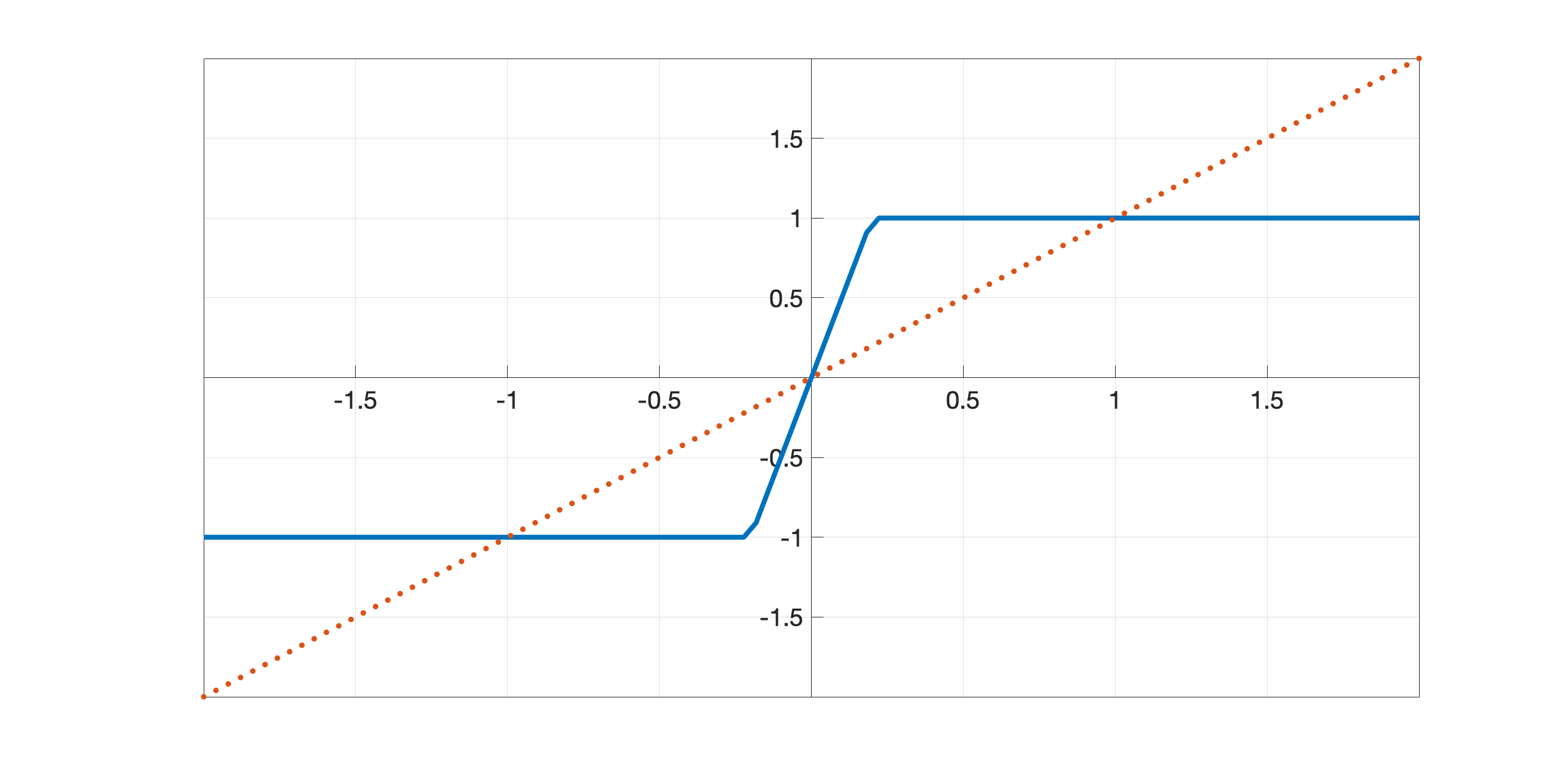
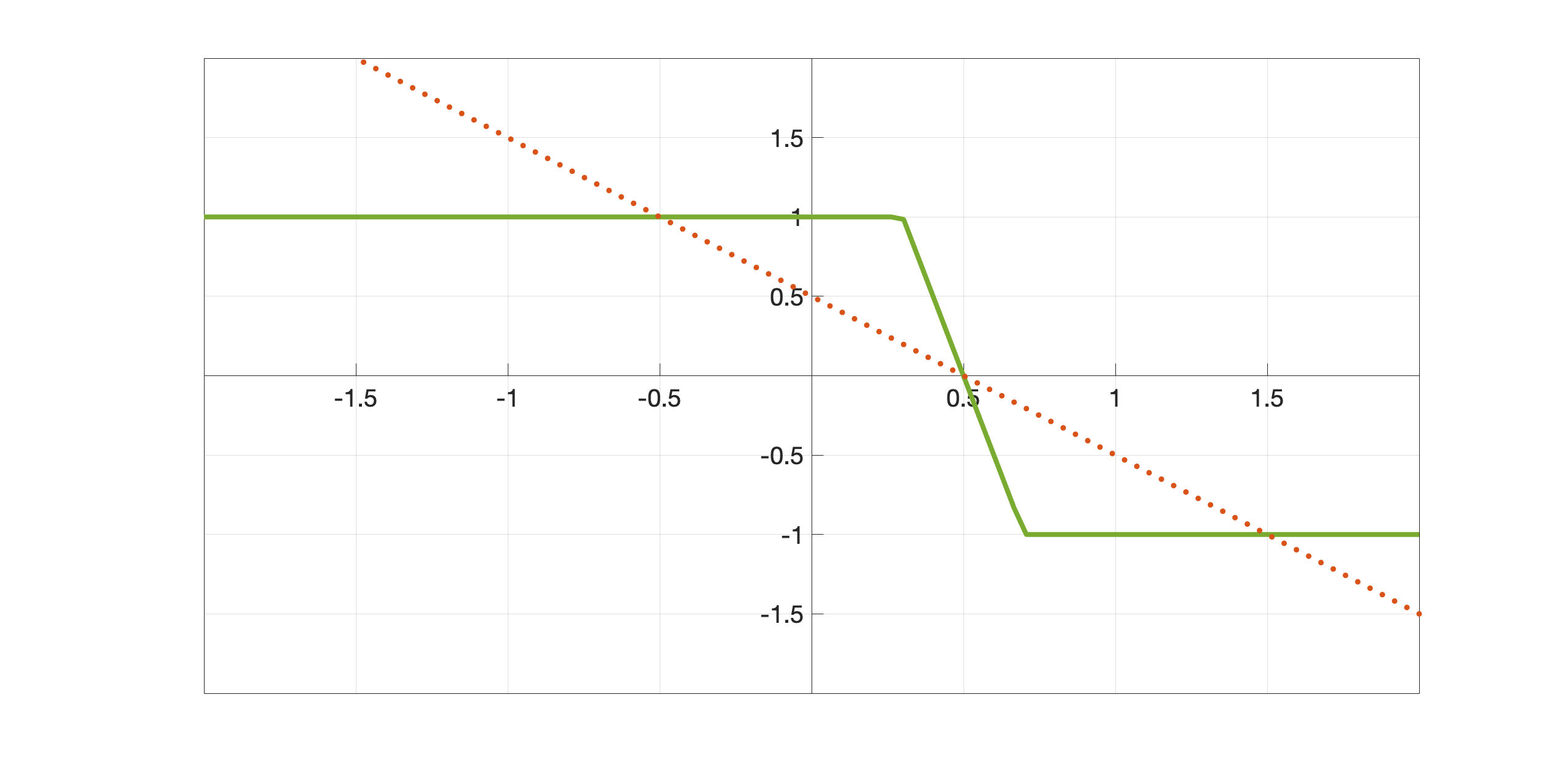
All the considered images are of size pixels, and take values in the interval in order to avoid out-of-range issues. We always consider discretised orientations, as done in [Boscain et al., 2018] for instance. As presented in Appendix B, the receptive profiles associated to the discretised orientations selected are obtained via cake wavelets [Bekkers et al., 2014], for which the frequency band bw is set to bw. The interaction kernel is taken to be a D or D Gaussian with standard deviation , the local mean average is obtained via Gaussian filtering with standard deviation . In our experiments we used the following two piece-wise linear functions as sigmoids:
| (2.10) |
with , see Figure 3. Note that , which will be used for LHE models, is odd and centered in zero while , which will be used for WC models, is shifted in and shows a reversed behaviour. This in fact corresponds to a change of sign in the integral terms of LHE models w.r.t. the WC ones, as discussed in Section 2.2.2.
Finally, the evolution stops when the relative distance between two successive iterations is smaller than a tolerance , which identifies convergence of the iterates to a stationary state.
3 Results
In this section, we present the results obtained by applying the four models described above to the visual illusions described in Section 2.1. Our objective is to understand the capability of these models to replicate the visual illusions under consideration. That is, we are interested in whether the output produced by the models qualitatively agrees with the human perception of the phenomena. We stress that our study is purely qualitative as it has to be intended as a proof of concept showing how Wilson-Cowan-type dynamics can be effectively used to replicate the perceptual effects due to the observation of visual illusions. We do not address here the match with empirical data since those depend on several experimental conditions for which a correspondence with the model parameters is not clear. A dedicated study on experiments motivated by psychophysics, addressing the validation of our models and, possibly, allowing for the creation of ground-truth references for a quantitative assessment is left for future research.
Due to the lack of a universal metric adapted to the task of assessing the replication of visual illusions, we will evaluate replication or lack thereof by presenting relevant line profiles, i.e., plots of brightness levels along a single row (line), of images produced by the four models in consideration (a common tool used by several brightness/lightness/color models before [Blakeslee et al., 2016, Otazu et al., 2008]). These lines are chosen as to cross a section of the image called target: A gray region in the image (or set of regions in the case of the Chevreul illusion), where the brightness illusion appears.
In all the results shown in this section, the original visual stimulus profile is represented as a blue dashed line. The line profiles of the output models are represented as solid red (LHE-2D), green (WC-2D), magenta (LHE-3D), and cyan (WC-3D) lines.
The parameters appearing in the models have been chosen independently for each illusion and each model, in order to obtain the best possible replication of the visual illusion. Here, by best-replication we mean that the extracted line-profiles correctly mimic the perceptual outcome from a qualitative point of view.The chosen parameters are presented in Table 1.
| WC-2D | LHE-2D | WC-3D | LHE-3D | |||||||||||||
| Illusion | ||||||||||||||||
| White | 10 | 20 | .7 | 1.4 | 10 | 50 | .7 | 1 | 20 | 30 | .7 | 1.4 | 2 | 50 | .7 | 1 |
| Brightness | 2 | 10 | .7 | 1.4 | 2 | 10 | .7 | 1 | 2 | 10 | .7 | 1.4 | 2 | 10 | .7 | 1 |
| Checkerboard | 10 | 70 | .7 | 1.4 | 10 | 70 | .7 | 1 | 10 | 70 | .7 | 1.4 | 10 | 70 | .7 | 1 |
| Chevreul | 2 | 5 | .7 | 1 | 2 | 10 | .7 | 1 | 2 | 40 | .5 | 1 | 5 | 7 | .7 | 1 |
| Chevreul canc. | 2 | 2 | .9 | 1 | 5 | 3 | .9 | 1 | 2 | 20 | .5 | 1.4 | 5 | 3 | .9 | 1 |
| Dungeon | 6 | 10 | .7 | 1.4 | 5 | 40 | .7 | 1 | 2 | 50 | .7 | 1.4 | 5 | 50 | .7 | 1 |
| Gratings | 2 | 6 | .7 | 1 | 2 | 6 | .7 | 1 | 2 | 6 | .7 | 1 | 2 | 6 | .7 | 1 |
| Hong-Shevell | 5 | 20 | .7 | 1 | 5 | .5 | .7 | 1 | 10 | 30 | .7 | 1 | 10 | 30 | .7 | 1 |
| Luminance | 2 | 6 | .7 | 1 | 2 | 6 | .7 | 1 | 2 | 6 | .7 | 1 | 2 | 6 | .7 | 1 |
| Poggendorff | ✗ | ✗ | ✗ | ✗ | ✗ | ✗ | ✗ | ✗ | ✗ | ✗ | ✗ | ✗ | 3 | 10 | .5 | 1 |
| Tilt | ✗ | ✗ | ✗ | ✗ | ✗ | ✗ | ✗ | ✗ | ✗ | ✗ | ✗ | ✗ | 15 | 20 | .7 | 1 |
3.1 Orientation-independent brightness illusions
Table 1 summarises the replication results obtained for the illusions described in Section 2.1: if the model replicates the illusion we indicate in the table the used parameters, otherwise a cross (✗) denotes no replication, i.e. the failure of the model to reproduce computational results corresponding to the visual perception of the considered illusion.
White’s illusion.
The chosen line profile for the plots in Fig. 4 corresponds to the central horizontal line of the image, which crosses both gray patches. As both plots show, all four models correctly predict the left target to be darker than the right one.
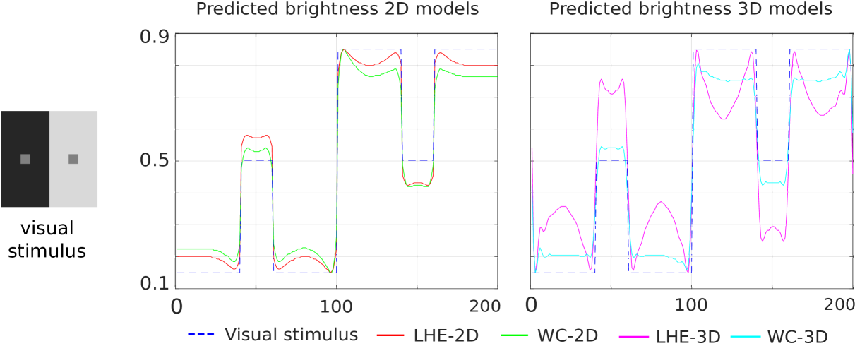
Simultaneous brightness contrast.
The plots in Fig. 5 show the line profiles of the central horizontal line of the image, which crosses the two gray squares. We see that our four models replicate this illusion (left square lighter than the right square). In both the 2D and the 3D case, we observe that LHE methods result in an enhanced contrast effect w.r.t. WC methods.
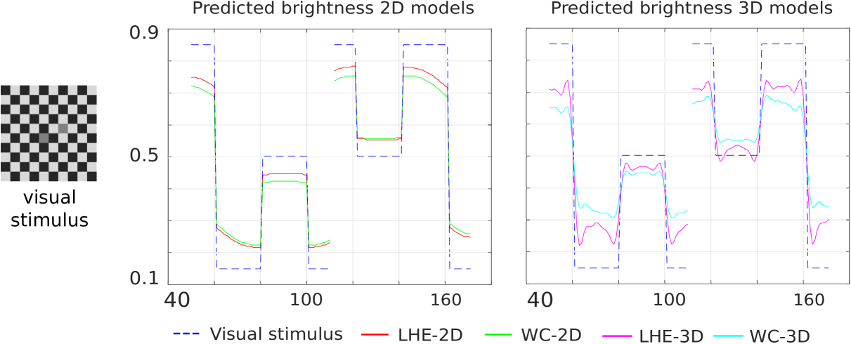
Checkerboard illusion.
The chosen line profiles for this illusion are the two horizontal lines crossing, respectively, the left gray target and the right one. In Fig. 6, we chose to plot the first half of the line profile corresponding to the left target and the second half of the one corresponding to the right target. The profiles of all the four models show replication of this illusion, by which the left target is perceived darker than the right one.
Chevreul illusion.
Fig. 7 presents the line profiles for the central horizontal line.All four models correctly replicate the perceived changes within each band.
.
Chevreul cancellation.
The line profiles for the central horizontal line are presented in Fig. 8. In this case all models are able to correctly replicate the effect, although in the case of (WC-2D) and (LHE-3D) the perceptual response is not perfect, due to the presence of some oscillations. We also remark that the correct replication of this illusion is extremely sensitive to the chosen parameters.
Dungeon illusion.
Profiles of the central section (3 middle squares) of each target are shown in Fig. 9. The first part of the plot (left to right) represents the profile of the rectangle on black background. The second plot shows the target on white background. As these profiles show, our four proposed models replicate human perception (first target is predicted as darker than the second). Nevertheless, the assimilation effect (target intensity goes towards surrounding) is stronger in the 3D models.
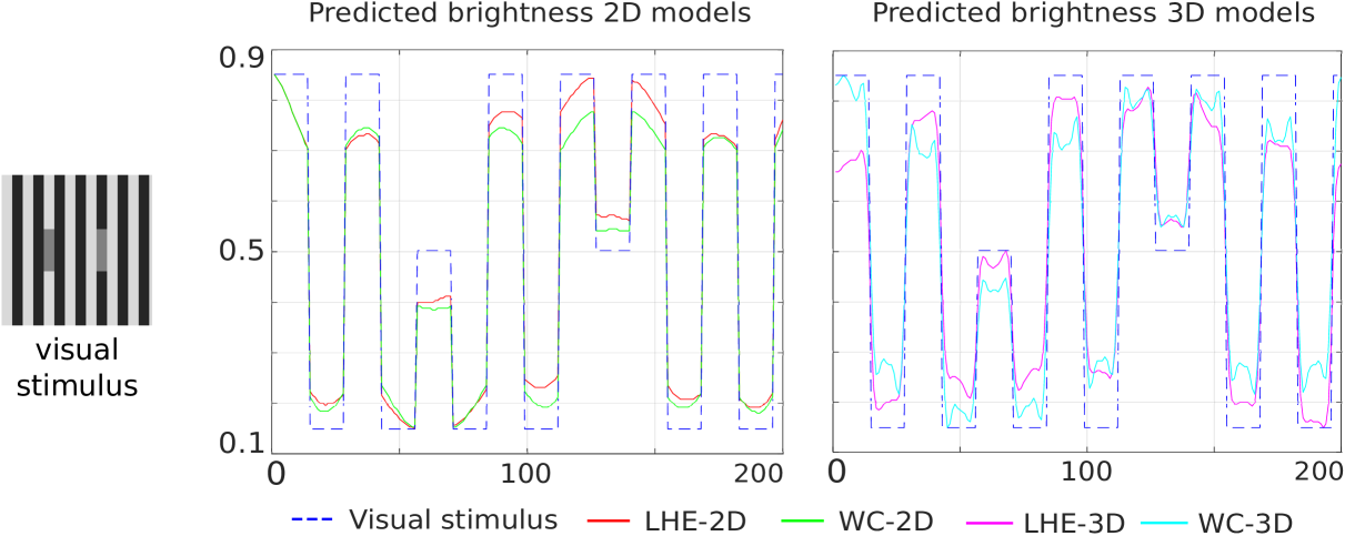
Grating induction.
In Fig. 10 the continuous and dashed blue lines respectively show the profile of the grating and of the central horizontal line row of the visual stimulus. Then, the line profiles of the central horizontal line of the outputs have been plotted. We observe that for both 2D and 3D models a counter-phase grating appears in the middle row, which successfully coincides with human perception. Notice that LHE methods have a higher amplitude in both cases.
Hong-Shevell illusion.
Fig. 11 shows the line profiles of the central horizontal line around the target (gray ring) neighbourhood rings in the first half of the image. As in the case of the Dungeon illusion, we present in the first half of the plot (left to right) the output of the first stimulus (light background) and in the second half the output of the second (dark background). We see how our four proposed models replicate the assimilation effect. Hence, the gray ring in the first image is predicted as brighter than the gray ring in the second visual stimulus.
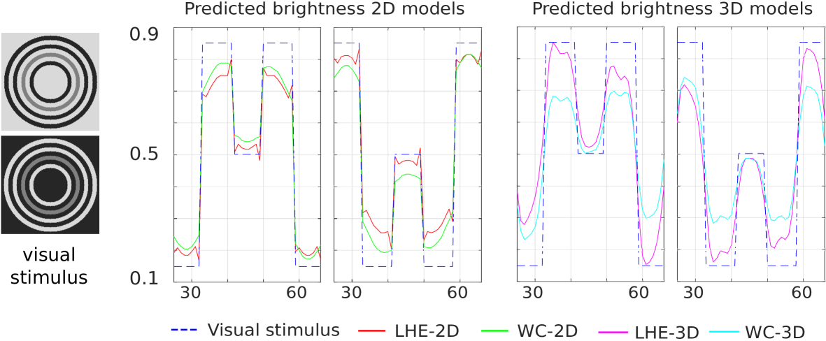
Luminance illusion.
Horizontal profiles crossing top left and right targets (gray circles) are depicted in Fig. 12. For each target our four models reconstruct the left target as brighter than the right one. Hence, all models correctly predict this contrast effect. In this case, LHE presents a higher contrast response in both responses (2D and 3D).
We observe that in all the considered brightness illusions both the 3D methods present neighbourhood-dependent oscillations.
3.2 Orientation-dependent illusions
Poggendorff illusion.
The output images and a zoom of the target gray middle area are presented in Fig. 13. In this case (WC-2D), (WC-3D), and (LHE-2D) are not able to completely replicate the illusion, since induced white lines on the gray area are not connected. On the other hand, (LHE-3D) successfully replicates the perceptual completion over the gray middle stripe.
Tilt illusion.
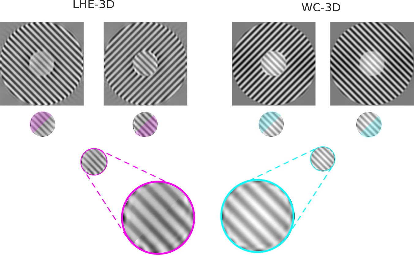
In Fig. 14 we present line profiles, for both visual stimuli, for a diagonal line starting at the bottom left corner of the image and ending at the top right one. In order to be able to correctly compare the two images, the line profile of the second image (from top to bottom) has been extracted after flipping the outer circle along the vertical axis, so that the responses to both stimulus have the same background. Although there is a noticeable effect, such as a reduction in contrast for the (WC-2D), the difference between the responses to the two stimuli is very mild for all models with the exception of (LHE-3D).
The fact that indeed this model is replicating the effect can be better appreciated looking at Fig. 15, which shows a composite of the inner circle for the responses to the two visual stimuli of the two orientation-dependent models. It is then evident that the (LHE-3D) model yields a stronger result than the (WC-3D) one. In fact, the former shows increased visibility (measured here as the contrast) for the half of the circle corresponding to the second stimulus than the one corresponding to the first stimulus. On the other hand, in the case of the (WC-3D) model (or of 2D models, not depicted here), the circle shows no difference among its two halves. This justifies our claim that the (LHE-3D) model can increase the visibility of the inner circle (replicate the illusion) based on the orientation of the outer circle.
4 Discussion
The results presented in the previous section show that the four models are able to reproduce several brightness illusions. Concerning orientation-dependent illusions we observe that, as expected, 2D models cannot reproduce them, while the only 3D model that correctly reproduces the perceptual outcome is the (LHE-3D). However we stress that determining replication or lack thereof in the Tilt illusion is subtle, as the observed effects are very mild.
As already mentioned, the parameters of the presented results are chosen independently from one illusion to the other in order to qualitatively optimise the perceptual replication in terms of suitable line profiles. Empirical observations show that the value of the model parameters involved are indeed related with the size of the target and the spatial frequency of the background. Nevertheless, if one settles for milder replications, it would be possible to choose more uniform parameters. For instance, this happens for the (WC-3D) model in the Chevreul and Chevreul cancellation illusions, which can be reproduced simultaneously with parameters and , although with less striking results.
Regarding the 3D models, we want to point out that we have chosen to use orientations whereas this number commonly takes values in the 12-18 range in the literature (e.g. [Scholl et al., 2013, Chariker et al., 2016, Pattadkal et al., 2018]). Our selection of 30 orientations is motivated by some preliminary tests (which we are not presenting here) showing that a coarser orientation discretisation seems not to be sufficient to reproduce most of the orientation-dependent illusions. As future research we will test whether or not a different selection of parameters allows to reproduce those illusions with less orientations, but we should also mention that some works in the literature actually use a high number of orientations in cortical models (e.g. 64 orientations in [Teich and Qian, 2010]).
Finally, we notice that the output of 3D models often shows oscillations. For some illusions (white and dungeon), the (WC-3D) model produces more oscillatory solutions than (LHE-3D), and for others (Chevreul brightness, grating induction, and luminace gradient), the (LHE-3D) have stronger oscillations than (WC-3D). The relation between the model parameters and possible dependence of the target surrounding is a matter of future research.
5 Conclusions and future work
We consider Wilson-Cowan-type models describing neuronal dynamics and apply them to the study of replication of brightness visual illusions.
We show that Wilson-Cowan equations are able to replicate a number of brightness illusions and that their variational modification, accounting for changes in the local contrast and performing local histogram equalisation, outperforms them. We consider also extensions of both models accounting for explicit local orientation dependence, in agreement with the architecture of V1. Although in the case of pure brightness illusions we found no real advantage in considering models taking into account orientations, these turned out to be necessary for the replication of two exemplary orientation-dependent illusions, which only the 3D LHE variational model is able to reproduce.
In order to understand and fully exploit the potential of the orientation-dependent LHE model, further research should be done. In particular, a more accurate modelling reflecting the actual structure of V1 should be addressed. This concerns first the lift operation, where the cake wavelet should be replaced by the more physiologically plausible Gabor filters, as well as the interaction weight which could be taken to be the anisotropic heat kernel of [Citti and Sarti, 2006, Sarti and Citti, 2015, Duits and Franken, 2010]. The design of appropriate psychophysics experiments testing the visual illusions considered in this work and their match with our models’ outputs is clearly a further important research direction, which would turn our qualitative study into a quantitative one. The problem of matching computational models of perception with psychophysical data is in fact not trivial, but necessary to provide insights about how visual perception works and to identify the computational parameters able to reproduce the perceptual bias induced by these phenomena.
Acknowledgements and Grants
M. B. would like to thank the organizers of the conference to celebrate Jack Cowan’s 50 years at the University of Chicago for their kind invitation to attend that meeting, which served as inspiration for this work, and also acknowledges the support of the European Union’s Horizon 2020 research and innovation programme under grant agreement number 761544 (project HDR4EU) and under grant agreement number 780470 (project SAUCE), and of the Spanish government and FEDER Fund, grant ref. PGC2018-099651-B-I00 (MCIU/AEI/FEDER, UE). L. C., V. F. and D. P. acknowledge the support of a public grant overseen by the French National Research Agency (ANR) as part of the Investissement d’avenir program, through the iCODE project funded by the IDEX Paris-Saclay, ANR-11-IDEX-0003-02 and of the research project LiftME funded by INS2I, CNRS. L. C. and V. F. acknowledge the support provided by the Fondation Mathématique Jacques Hadamard. V. F. acknowledges the support received from the European Union’s Horizon 2020 research and innovation programme under the Marie Skłodowska-Curie grant No 794592. V. F. and D. P. also acknowledge the support of ANR-15-CE40-0018 project SRGI - Sub-Riemannian Geometry and Interactions. B. F. acknowledges the support of the Fondation Asile des Aveugles.
Disclosures
All authors declare that there is no commercial relationship relevant to the subject matter of presentation.
Author contributions
All authors equally contributed to this work.
Appendix A Non-variational nature of Wilson-Cowan equation
In this section we show that, for non-trivial choices of weight and sigmoid functions, Wilson-Cowan equations do not admit a variational formulation.
For the sake of simplicity, we will consider only a finite dimensional variant of Wilson-Cowan equations, with constant input. Namely, for , we consider
| (A.1) |
Here, is the input, is a parameter, is any function (we denoted for ), and is a symmetric interaction kernel. For a proof in the infinite-dimensional setting we refer to [Bertalmío et al., 2019b]
Equation (A.1) admits a variational formulation if it can be written as the steepest descent associated with a functional , i.e.,
| (A.2) |
We have the following.
Theorem.
Proof.
Writing (A.1) and (A.2) componentwise, we find the following relation for :
By differentiating again the above, and letting denote the Kroenecker delta symbol, we have
| (A.3) |
Namely, . Assume that is not a diagonal matrix. Then, since both the Hessian matrix and are symmetric, by choosing such that we get
| (A.4) |
This clearly implies that is constant, thus showing that must be an affine function. ∎
We observe that the above reasoning does not apply to the LHE algorithm. Indeed, the discrete form of the latter is
| (LHE) |
Then, the corresponding variational equation (for and ) is
| (A.5) |
This yields
| (A.6) |
This does not contradict the symmetry of the Hessian, as was chosen to be odd an thus is even. Indeed, we know by [Bertalmío and Cowan, 2009] that we can let
| (A.7) |
where is such that .
Appendix B Encoding orientation-dependence via cortical-inspired models
Orientation dependence of the visual stimulus is encoded via cortical inspired techniques, following e.g., [Citti and Sarti, 2006, Duits and Franken, 2010, Petitot, 2017, Prandi and Gauthier, 2017, Bohi et al., 2017]. The main idea at the base of these works goes back to the 1959 paper [Hubel and Wiesel, 1959] by Hubel and Wiesel (Nobel prize in 1981) who discovered the so-called hypercolumn functional architecture of the visual cortex V1. Following [Hubel and Wiesel, 1959], each neuron in V1 detects couples where is a retinal position and is a direction at . Orientation preferences are then organised in hypercolumns over the retinal position , see [Petitot, 2017, Section 2].
Let be the visual plane. To a visual stimulus is associated a cortical activation such that encodes the response of the neuron . Letting be the receptive profile (RP) of the neuron , such response is assumed to be given by
| (B.1) |
Motivated by neuro-phyisiological evidence, we assume that RPs of different neurons are “deducible” one from the other via a linear transformation. As detailed in [Duits and Franken, 2010, Prandi and Gauthier, 2017], see also [Bertalmío et al., 2019a, Section 3.1], this amounts to the fact that the linear operator is a continuous wavelet transform (also called invertible orientation score transform). That is, there exists a mother wavelet such that . Here, denotes the standard convolution on and is the counter-clock-wise rotation of angle . Notice that, although images are functions of with values in , it is in general not true that .
Concerning the choice of the mother wavelet, we remark that neuro-physiological evidence suggests that a good fit for the RPs is given by Gabor filters, whose Fourier transform is the product of a Gaussian with an oriented plane wave [Daugman, 1985]. However, these filters are quite challenging to invert, and are parametrised on a bigger space than , which takes into account also the frequency of the plane wave and not only its orientation. For this reason, in this work we instead considered cake wavelets, introduced in [Duits et al., 2007, Bekkers et al., 2014]. These are obtained via a mother wavelet whose support in the Fourier domain is concentrated on a fixed slice, depending on the number of orientations one aims to consider in the numerical implementation. For the sake of integrability, the Fourier transform of this mother wavelet is then smoothly cut off via a low-pass filtering, see [Bekkers et al., 2014, Section 2.3] for details. Observe, however, that, since we are considering orientations on and not directions on , we choose a non-oriented version of the mother wavelet, given by , in the notations of [Bekkers et al., 2014].
An important feature of cake wavelets is that, in order to recover the original stimulus from its cortical activation, it suffices to simply “project” the cortical activations along hypercolumns. This yields
| (B.2) |
This justify the assumption, implicit in equation (2.9), that the projection of a cortical activation (not necessarily given by a visual stimulus) to the visual plane is given by
| (B.3) |
References
- [Adini et al., 1997] Adini, Y., Sagi, D., and Tsodyks, M. (1997). Excitatory–inhibitory network in the visual cortex: Psychophysical evidence. Proceedings of the National Academy of Sciences, 94(19):10426–10431.
- [Atick, 1992] Atick, J. J. (1992). Could information theory provide an ecological theory of sensory processing? Network: Computation in Neural Systems, 3(2):213–251.
- [Attneave, 1954] Attneave, F. (1954). Some informational aspects of visual perception. Psychological review, 61(3):183.
- [Barlow et al., 1961] Barlow, H. B. et al. (1961). Possible principles underlying the transformation of sensory messages. Sensory communication, 1:217–234.
- [Bekkers et al., 2014] Bekkers, E., Duits, R., Berendschot, T., and ter Haar Romeny, B. (2014). A multi-orientation analysis approach to retinal vessel tracking. JMIV, 49(3):583–610.
- [Benucci et al., 2013] Benucci, A., Saleem, A. B., and Carandini, M. (2013). Adaptation maintains population homeostasis in primary visual cortex. Nature neuroscience, 16(6):724.
- [Bertalmío, 2014] Bertalmío, M. (2014). From image processing to computational neuroscience: a neural model based on histogram equalization. Front. Comput. Neurosc., 8:71.
- [Bertalmío et al., 2019a] Bertalmío, M., Calatroni, L., Franceschi, V., Franceschiello, B., and Prandi, D. (2019a). A cortical-inspired model for orientation-dependent contrast perception: A link with Wilson-Cowan equations. In Lellmann, J., Burger, M., and Modersitzki, J., editors, Scale Space and Variational Methods in Computer Vision, pages 472–484, Cham. Springer International Publishing.
- [Bertalmío et al., 2019b] Bertalmío, M., Calatroni, L., Franceschi, V., Franceschiello, B., and Prandi, D. (2019b). Cortical-inspired Wilson-Cowan-type equations for orientation-dependent contrast perception modelling. arXiv preprint: https://arxiv.org/abs/1910.06808.
- [Bertalmío et al., 2007] Bertalmío, M., Caselles, V., Provenzi, E., and Rizzi, A. (2007). Perceptual color correction through variational techniques. IEEE T. Image Process., 16(4):1058–1072.
- [Bertalmío and Cowan, 2009] Bertalmío, M. and Cowan, J. D. (2009). Implementing the retinex algorithm with wilson–cowan equations. Journal of Physiology-Paris, 103(1-2):69–72.
- [Bertalmío and Cowan, 2009] Bertalmío, M. and Cowan, J. D. (2009). Implementing the retinex algorithm with Wilson-Cowan equations. J. Physiol. Paris, 103(1):69 – 72.
- [Bertalmío et al., 2017] Bertalmío, M., Cyriac, P., Batard, T., Martinez-Garcia, M., and Malo, J. (2017). The wilson-cowan model describes contrast response and subjective distortion. J Vision, 17(10):657–657.
- [Beurle and Matthews, 1956] Beurle, R. L. and Matthews, B. H. C. (1956). Properties of a mass of cells capable of regenerating pulses. Philosophical Transactions of the Royal Society of London. Series B, Biological Sciences, 240(669):55–94.
- [Bezanson et al., 2017] Bezanson, J., Edelman, A., Karpinski, S., and Shah, V. B. (2017). Julia: A fresh approach to numerical computing. SIAM review, 59(1):65–98.
- [Blakeslee et al., 2016] Blakeslee, B., Cope, D., and McCourt, M. E. (2016). The oriented difference of gaussians (ODOG) model of brightness perception: Overview and executable Mathematica notebooks. Behav. Res. Methods, 48(1):306–312.
- [Bohi et al., 2017] Bohi, A., Prandi, D., Guis, V., Bouchara, F., and Gauthier, J.-P. (2017). Fourier descriptors based on the structure of the human primary visual cortex with applications to object recognition. Journal of Mathematical Imaging and Vision, 57(1):117–133.
- [Boscain et al., 2018] Boscain, U. V., Chertovskih, R., Gauthier, J.-P., Prandi, D., and Remizov, A. (2018). Highly corrupted image inpainting through hypoelliptic diffusion. Journal of Mathematical Imaging and Vision, 60(8):1231–1245.
- [Bressan, 2001] Bressan, P. (2001). Explaining lightness illusions. Perception, 30(9):1031–1046.
- [Brucke, 1865] Brucke, E. (1865). uber erganzungs und contrasfarben. Wiener Sitzungsber, 51.
- [Chariker et al., 2016] Chariker, L., Shapley, R., and Young, L.-S. (2016). Orientation selectivity from very sparse lgn inputs in a comprehensive model of macaque v1 cortex. Journal of Neuroscience, 36(49):12368–12384.
- [Citti and Sarti, 2006] Citti, G. and Sarti, A. (2006). A cortical based model of perceptual completion in the roto-translation space. JMIV, 24(3):307–326.
- [Cowan et al., 2016] Cowan, J. D., Neuman, J., and van Drongelen, W. (2016). Wilson–cowan equations for neocortical dynamics. The Journal of Mathematical Neuroscience, 6(1):1.
- [Daugman, 1985] Daugman, J. G. (1985). Uncertainty relation for resolution in space, spatial frequency, and orientation optimized by two-dimensional visual cortical filters. J. Opt. Soc. Am. A, 2(7):1160–1169.
- [DeValois and DeValois, 1990] DeValois, R. L. and DeValois, K. K. (1990). Spatial vision. Oxford university press.
- [Duits et al., 2007] Duits, R., Felsberg, M., Granlund, G., and ter Haar Romeny, B. (2007). Image analysis and reconstruction using a wavelet transform constructed from a reducible representation of the euclidean motion group. International Journal of Computer Vision, 72(1):79–102.
- [Duits and Franken, 2010] Duits, R. and Franken, E. (2010). Left-invariant parabolic evolutions on and contour enhancement via invertible orientation scores. Part I: linear left-invariant diffusion equations on . Quart. Appl. Math., 68(2):255–292.
- [Eagleman, 1959] Eagleman, D. M. (1959). Visual illusions and neurobiology. Nature reviews Neuroscience, (2):920–926 (2001).
- [Ernst et al., 2016] Ernst, U. A., Schiffer, A., Persike, M., and Meinhardt, G. (2016). Contextual interactions in grating plaid configurations are explained by natural image statistics and neural modeling. Frontiers in systems neuroscience, 10:78.
- [Fairhall et al., 2001] Fairhall, A. L., Lewen, G. D., Bialek, W., and van Steveninck, R. R. d. R. (2001). Efficiency and ambiguity in an adaptive neural code. Nature, 412(6849):787.
- [Faugeras, 2009] Faugeras, O. (2009). A constructive mean-field analysis of multi population neural networks with random synaptic weights and stochastic inputs. Frontiers in Computational Neuroscience, 3.
- [French, 2004] French, D. (2004). Identification of a free energy functional in an integro-differential equation model for neuronal network activity. Applied Mathematics Letters, 17(9):1047 – 1051.
- [Geier and Hudák, 2011] Geier, J. and Hudák, M. (2011). Changing the chevreul illusion by a background luminance ramp: lateral inhibition fails at its traditional stronghold-a psychophysical refutation. PloS One, 6(10):e26062.
- [Herzog et al., 2003] Herzog, M. H., Ernst, U. A., Etzold, A., and Eurich, C. W. (2003). Local interactions in neural networks explain global effects in gestalt processing and masking. Neural Computation, 15(9):2091–2113.
- [Hong and Shevell, 2004] Hong, S. W. and Shevell, S. K. (2004). Brightness contrast and assimilation from patterned inducing backgrounds. Vision Research, 44(1):35–43.
- [Hubel and Wiesel, 1959] Hubel, D. and Wiesel, T. (1959). Receptive fields of single neurones in the cat’s striate cortex. The Journal of physiology, 148(3):574–591.
- [Kingdom, 2011] Kingdom, F. A. (2011). Lightness, brightness and transparency: A quarter century of new ideas, captivating demonstrations and unrelenting controversy. Vision Research, 51(7):652–673.
- [Kitaoka, 2006] Kitaoka, A. (2006). Adelson’s checker-shadow illusion-like gradation lightness illusion. http://www.psy.ritsumei.ac.jp/~akitaoka/gilchrist2006mytalke.html. Accessed: 2018-11-03.
- [Mante et al., 2005] Mante, V., Frazor, R. A., Bonin, V., Geisler, W. S., and Carandini, M. (2005). Independence of luminance and contrast in natural scenes and in the early visual system. Nature neuroscience, 8(12):1690.
- [McCourt, 1982] McCourt, M. E. (1982). A spatial frequency dependent grating-induction effect. Vision Research, 22(1):119–134.
- [Meister and Berry, 1999] Meister, M. and Berry, M. J. (1999). The neural code of the retina. Neuron, 22(3):435–450.
- [Murray and Herrmann, 2013] Murray, M. M. and Herrmann, C. (2013). Illusory contours: a window onto the neurophysiology of constructing perception. Trends Cogn Sci., (17(9)):471–81.
- [Olshausen and Field, 2000] Olshausen, B. A. and Field, D. J. (2000). Vision and the coding of natural images: The human brain may hold the secrets to the best image-compression algorithms. AmSci, 88(3):238–245.
- [Otazu et al., 2008] Otazu, X., Vanrell, M., and Parraga, C. A. (2008). Multiresolution wavelet framework models brightness induction effects. Vis. Res., 48(5):733 – 751.
- [Pattadkal et al., 2018] Pattadkal, J. J., Mato, G., van Vreeswijk, C., Priebe, N. J., and Hansel, D. (2018). Emergent orientation selectivity from random networks in mouse visual cortex. Cell reports, 24(8):2042–2050.
- [Petitot, 2017] Petitot, J. (2017). Elements of Neurogeometry: Functional Architectures of Vision. Lecture Notes in Morphogenesis. Springer International Publishing.
- [Prandi and Gauthier, 2017] Prandi, D. and Gauthier, J.-P. (2017). A semidiscrete version of the Petitot model as a plausible model for anthropomorphic image reconstruction and pattern recognition. SpringerBriefs in Mathematics. Springer International Publishing, Cham.
- [Purves et al., 2008] Purves, D., Wojtach, W. T., and Howe, C. (2008). Visual illusions: An Empirical Explanation. Scholarpedia, 3(6):3706. revision #89112.
- [Ratliff, 1965] Ratliff, F. (1965). Mach bands: quantitative studies on neural networks. Holden-Day, San Francisco London Amsterdam.
- [Sarti and Citti, 2015] Sarti, A. and Citti, G. (2015). The constitution of visual perceptual units in the functional architecture of V1. J. comput. neurosc., 38(2):285–300.
- [Scholl et al., 2013] Scholl, B., Tan, A. Y., Corey, J., and Priebe, N. J. (2013). Emergence of orientation selectivity in the mammalian visual pathway. Journal of Neuroscience, 33(26):10616–10624.
- [Shapiro and Todorovic, 2016] Shapiro, A. G. and Todorovic, D. (2016). The Oxford compendium of visual illusions. Oxford University Press.
- [Smirnakis et al., 1997] Smirnakis, S. M., Berry, M. J., Warland, D. K., Bialek, W., and Meister, M. (1997). Adaptation of retinal processing to image contrast and spatial scale. Nature, 386(6620):69.
- [Teich and Qian, 2010] Teich, A. F. and Qian, N. (2010). V1 orientation plasticity is explained by broadly tuned feedforward inputs and intracortical sharpening. Visual neuroscience, 27(1-2):57–73.
- [Weintraub and Krantz, 1971] Weintraub, D. J. and Krantz, D. H. (1971). The Poggendorff illusion: amputations, rotations, and other perturbations. Attent. Percept. Psycho., 10(4):257–264.
- [White, 1979] White, M. (1979). A new effect of pattern on perceived lightness. Perception, 8(4):413–416.
- [Wilson, 2003] Wilson, H. R. (2003). Computational evidence for a rivalry hierarchy in vision. Proceedings of the National Academy of Sciences, 100(24):14499–14503.
- [Wilson, 2007] Wilson, H. R. (2007). Minimal physiological conditions for binocular rivalry and rivalry memory. Vision Research, 47(21):2741 – 2750.
- [Wilson, 2017] Wilson, H. R. (2017). Binocular contrast, stereopsis, and rivalry: Toward a dynamical synthesis. Vision Research, 140:89–95.
- [Wilson and Cowan, 1972] Wilson, H. R. and Cowan, J. D. (1972). Excitatory and inhibitory interactions in localized populations of model neurons. BioPhys. J., 12(1).
- [Wilson and Cowan, 1973] Wilson, H. R. and Cowan, J. D. (1973). A mathematical theory of the functional dynamics of cortical and thalamic nervous tissue. Kybernetik, 13(2):55–80.