Vortex motion and flux-flow resistivity in dirty multiband superconductors

Mihail Silaev Department of Theoretical Physics, The Royal Institute of Technology, Stockholm, SE-10691 Sweden Artjom Vargunin Department of Theoretical Physics, The Royal Institute of Technology, Stockholm, SE-10691 Sweden Institute of Physics, University of Tartu, Tartu, EE-50411, Estonia

(August 7, 2025)

Abstract

The conductivity of vortex lattices in multiband superconductors with high concentration of impurities is calculated based on microscopic kinetic theory. Both the limits of high and low fields are considered, when the magnetic induction is close to or much smaller than the critical field strength $H_{c2}$ , respectively. It is shown that in contrast to single-band superconductors the resistive properties are not universal but depend on the pairing constants and ratios of diffusivities in different bands. The low-field magneto-resistance can strongly exceed Bardeen-Stephen estimation in a quantitative agreement with experimental data for two-band superconductor MgB₂.

I Introduction

Recent transport experiments reveal quite unusual behaviour of the flux-flow resistive states in multiband superconductors FluxFlowExperimentsFeAs1 ; FluxFlowExperimentsFeAs2 ; FluxFlowExperimentsFeAs3 ; FluxFlowExperimentsFeAs4 ; FluxFlowExperimentsFeAs5 ; FluxFlowExperimentsMgB2 . The magnetic field dependencies of flux-flow resistivity $\rho_{f}(B)$ were found to be qualitatively different from that observed in single-band superconductorsExperimentKim . This behaviour is not explained by the theories developed in previous works. BS ; GorkovKopnin1 ; GorkovKopnin2 ; MakiCaroli ; Thompson ; Ebisawa ; Schmid

Vortex motion in conventional type-II superconductors have been investigated for several decades. Flux-flow experiments in single-band superconductors at low temperatures and magnetic fieldsExperimentKim are well described by the Bardeen-Stephen (BS) theoryBS . In this regime the flux-flow resistivity is given by the linear magnetic field dependence

\rho_{f}/\rho_{n}=\beta^{-1}B/H_{c2},

(1)

where $\rho_{n}$ is the normal state resistivity, $B$ is an average magnetic induction, $H_{c2}$ is the second critical field and $\beta\approx 1$ . The BS law is in the qualitative agreement with the results obtained based on the microscopic theory for dirty superconductorsGorkovKopnin1 . At larger magnetic fields the dependence $\rho_{f}(B)$ becomes essentially non-linearExperimentKim ; Fogel . At elevated temperatures the significant growth of $\beta$ results in the suppressed magneto-resistivity as compared to the BS value GorkovKopnin2 ; OvchinnikovJETP .

In strong magnetic fields $H_{c2}-B\ll H_{c2}$ the motion of dense vortex lattices has been extensively studied with the help of linear response theory MakiCaroli ; Thompson ; Ebisawa . In these works the slope of flux-flow resistivity

S=(H_{c2}/\rho_{n})(d\rho_{f}/dB)

(2)

has been shown to have a universal temperature dependence in the dirty limit. It is characterized by a monotonic increase from $S(T=0)=1.72$ to $S(T=T_{c})=5$ Thompson . This behaviour was confirmed by accurate high-field measurements in Pb-In alloysExperimentThompson . The deviation at elevated temperatures near $T_{c}$ were explained by depairing due to the spin-flip and electron-phonon scatteringLarkinOvchinnikov .

In contrast to the conventional behaviour described above, many multiband superconductorsFluxFlowExperimentsFeAs1 ; FluxFlowExperimentsFeAs2 ; FluxFlowExperimentsFeAs3 ; FluxFlowExperimentsFeAs4 ; FluxFlowExperimentsFeAs5 including MgB₂ FluxFlowExperimentsMgB2 were found to have the flux-flow resistivity larger than the BS value $\rho_{f}/\rho_{n}>B/H_{c2}$ . The experimentally found dependencies $\rho_{f}(B)$ have a steeper growth in the low-field region with an enhanced magneto-resistance characterized by $\beta<1$ and a smaller slope $S<1$ at $B=H_{c2}$ FluxFlowExperimentsMgB2 , which is not described by the single-band theoryThompson .

The existing theories of flux-flow states cannot be straightforwardly applied to multiband superconductors. In these systems vortices have a composite structure consisting of multiple singularities corresponding to the order parameter phase windings in different superconducting bands. In equilibrium an isolated composite vortex is a bound state of several co-centred fractional vortices babaev2 . They can split however under the action of fluctuationsbabaev3 , interaction with other vortices and sample boundaries dao ; silaev or due to external drivelin . In particular it was shown that the moving composite vortices can split into separate fractional vortices and even dissociate in a non-linear regime provided the interband pairing is sufficiently smalllin . It is natural to expect that vortex splitting should have a profound effect on the flux-flow resistivity especially at high fields when the flux-flow resistivity is strongly affected by the distortions of the moving vortex latticeMakiCaroli ; Thompson ; Ebisawa . As will be shown below, the well-known solutionSchmid describing moving vortex lattice is not applicable to describe multiband systems since the distortion generically splits the sublattices of fractional vortices. In the present paper we develop a theoretical framework to take into account this effect and calculate the conductivity corrections. For that one needs to know the Maki parameter also known as a generalized Ginzbirg-Landau parameter $\kappa_{2}$ which determines in particular the order parameter density as a function of magnetic field near $H_{c2}$ MakiCaroli . Recently this parameter has been calculated for multiband superconductorsSilaevKappa2 .

To obtain a complete picture of the flux-flow conductivity behaviour in multiband systems we consider also the regime of small magnetic fields, when a picture of isolated moving vortices is an adequate descriptionGorkovKopnin1 . Based on the kinetic theory we calculate the coefficient $\beta$ which characterizes the initial slope of the magnetoresistance. Applying the combination of the results in two limiting cases of small and high magnetic fields it is possible to fit the experimental curves $\rho_{f}(B)$ for multiband superconductors with known pairing interactions such as MgB₂.

The model of dirty-limit superconductors assumed in the present work is appropriate for a certain class of multiband materials including MgB₂GurevichMgB2 ; KoshelevGolubovHc2 and iron-pnictidesGurevichFeAsNature . In single crystals of MgB₂ the de Haas-van Alphen data dHvAMgB2 and thermal conductivity measurements ThCondMgB2 suggest the borderline regime when one of the superconducting bands is moderately clean and the other one is moderately dirtyKoshelevGolubovHc2 . Scanning tunnel microscopy shows absence of zero-bias anomaly inside vortex cores which is typical for dirty superconductorsSTMMgB2 . Impurities at high concentration can be introduced in MgB₂ on demand during the preparation process producing non-trivial magnetic properties which have been intensively studied recently GurevichMgB2 ; MgB2Ex1 ; MgB2Ex2 ; MgB2Ex3 ; MgB2Ex4 .

The structure of this paper is as follows. In Sec.II we introduce the Keldysh-Usadel description of the kinetic processes in dirty multiband superconductors. Here the basic components of the kinetic theory are discussed including kinetic equations, self-consistency equations for the order parameter and current as well as a general expression for the viscous force acting on the moving vortices. The flux-flow conductivity at high magnetic fields is calculated in Sec.III taking into account the splitting of fractional vortex sublattices. The case of low fields is considered in Sec.IV. Quantitative comparison of theoretical results with flux-flow resistivity measurements in MgB₂ FluxFlowExperimentsMgB2 is discussed in Sec. V. The work summary is given in Sec.(VI).

II Kinetic equations and forces acting on the moving vortex line

We consider multiband superconductors in a dirty limit when the kinetics and spectral properties are described by the Keldysh-Usadel theory. For the single band case the theory of vortex motion in diffusive superconductors was developed in works GorkovKopnin1 ; GorkovKopnin2 ; LarkinOvchinnikov ; Thompson . Here we generalize their theory to the multiband case.

The quasiclassical GF in each band is defined as

\check{g}_{k}=\left(\begin{array}[]{cc}\hat{g}^{R}_{k}&\hat{g}^{K}_{k}\\ 0&\hat{g}^{A}_{k}\\ \end{array}\right)\;,

(3)

where $g^{K}_{k}$ is the (2 $\times$ 2 matrix) Keldysh component and $\hat{g}^{R(A)}_{k}$ is the retarded (advanced) GF, $k$ is the band index. In dirty superconductors the matrix $\check{g}$ obeys the Usadel equation

\{\tau_{3}\partial_{t},\check{g}_{k}\}_{t}=D_{k}\hat{\partial}_{\bf r}(\check{g}_{k}\circ\hat{\partial}_{\bf r}\check{g}_{k})+[\hat{H}_{k},\check{g}_{k}]_{t}-i[\check{\Sigma}^{ph},\check{g}_{k}]_{t}

(4)

where $D_{k}$ is the diffusion constant, and $\hat{H}_{k}({\bm{r}},t)=i\hat{\Delta}_{k}$ where $\hat{\Delta}_{k}(t)=i|\Delta_{k}|\tau_{2}e^{-i\theta_{k}\tau_{3}}$ is the gap operator in $k$ -th band. We use from the beginning the temporal gauge where the scalar potential is zero $\Phi=0$ with and additional constraint that in equilibrium the vector potential is time-independent and satisfies $\nabla\cdot\bm{A}=0$ . In Eq.(4) the covariant differential superoperator is defined by

\hat{\partial}_{\bf r}\hat{g}_{k}=\nabla\hat{g}_{k}-ie\left[\tau_{3}{\bm{A}},\hat{g}_{k}\right]_{t}.

The gap in each band is determined by self consistency equation

\Delta_{k}(t,\bm{r})=\frac{\pi}{2}\lambda_{kj}(\hat{g}^{K}_{j})_{12}(t_{1,2}=t,\bm{r}).

(5)

Here $\hat{\Lambda}$ is the coupling matrix satisfying symmetry relations $\nu_{1}\lambda_{12}=\nu_{2}\lambda_{21}$ , where $\nu_{k}$ is the DOS. The electric current density is given by

{\bm{j}}(t,\bm{r})=\frac{\pi e}{2}\sum_{k}\nu_{k}D_{k}{\rm Tr}(\check{g}_{k}\circ\hat{\partial}_{\bm{r}}\check{g}_{k})^{K}(t_{1,2}=t,\bm{r})

(6)

We define the commutator operator as $[X,g]_{t}=X(t_{1})g(t_{1},t_{2})-g(t_{1},t_{2})X(t_{2})$ , similarly for anticommutator $\{,\}_{t}$ . We introduce the symbolic product operator $(A\circ B)(t_{1},t_{2})=\int dtA(t_{1},t)B(t,t_{2})$ .

The Keldysh-Usadel Eq. (4) is complemented by the normalization condition $(\check{g}_{k}\circ\check{g}_{k})(t_{1},t_{2})=\check{\delta}(t_{1}-t_{2})$ which allows to introduce parametrization of the Keldysh component in terms of the distribution function

	$\displaystyle\hat{g}^{K}_{k}=\hat{g}^{R}_{k}\circ\hat{f}^{(k)}-\hat{f}^{(k)}\circ\hat{g}^{A}_{k}$		(7)
	$\displaystyle\hat{f}^{(k)}=f^{(k)}_{L}\tau_{0}+f^{(k)}_{T}\tau_{3}.$		(8)

To proceed we introduce the mixed representation in the time-energy domain as follows $g_{k}(t_{1},t_{2})=\int_{-\infty}^{\infty}g_{k}(\varepsilon,t)e^{-i\varepsilon(t_{1}-t_{2})}d\varepsilon/(2\pi)$ , where $t=(t_{1}+t_{2})/2$ .

We employ Larkin-Ovchinnikov theoryLarkinOvchinnikov ; KopninBook to calculate the force acting on the moving vortex line. In multiband superconductors the force is given by a linear superposition of contributions from different bandsKopninBook ; LarkinOvchinnikov

	$\displaystyle{\bm{F}}_{env}=\sum_{k}{\bm{F}}^{(k)}_{env}+\frac{1}{c}\int d^{2}{\bm{r}}{\bm{H}}\times{\bm{j}}^{(nst)}$		(9)
	$\displaystyle{\bm{F}}^{(k)}_{env}=\nu_{k}\int d^{2}{\bm{r}}\int_{-\infty}^{\infty}\frac{d\varepsilon}{4}{\rm Tr}(\hat{g}^{nst}_{k}\hat{\partial}_{\bm{r}}\hat{\Delta}_{k})$		(10)

where the covariant differential superoperator is given by $\hat{\partial}_{\bf r}\hat{\Delta}_{k}=\nabla\hat{\Delta}_{k}-ie\left[\tau_{3}{\bm{A}},\hat{\Delta}_{k}\right]$ . Eqs.(9,10 ) contain a non-stationary part of the electric current density ${\bm{j}}^{(nst)}$ and the Keldysh component of a non-stationary Green’s function $\hat{g}^{nst}_{k}$ which can be expressed through the gradient expansion as follows

	$\displaystyle\hat{g}^{nst}_{k}=-\frac{i}{2}\partial_{t}(\hat{g}^{R}_{k}+\hat{g}^{A}_{k})\partial_{\varepsilon}f_{0}+$		(11)
	$\displaystyle(\hat{g}^{R}_{k}-\hat{g}^{A}_{k})f^{(k)}_{L}+(\hat{g}^{R}_{k}\tau_{3}-\tau_{3}\hat{g}^{A}_{k})f^{(k)}_{T}.$		(12)

Keeping the first order non-equilibrium terms and neglecting the electron-phonon relaxation in Eq.(4) we obtain a system of two coupled kinetic equation that determine both the transverse $f_{T}^{(k)}$ and longitudinal $f_{L}^{(k)}$ distribution function components

		$\displaystyle\nabla({\cal D}_{T}^{(k)}\nabla f_{T}^{(k)})+{\bm{j}}_{e}^{(k)}\cdot\nabla f_{L}^{(k)}+2i{\rm Tr}[(\hat{g}^{R}_{k}+\hat{g}^{A}_{k})\hat{\Delta}_{k}]f_{T}^{(k)}=$
		$\displaystyle\partial_{\varepsilon}f_{0}{\rm Tr}[\tau_{3}\partial_{t}\hat{\Delta}_{k}(\hat{g}^{R}_{k}+\hat{g}^{A}_{k})]-e\partial_{\varepsilon}f_{0}\nabla\cdot({\cal D}_{T}^{(k)}{\bm{E}}),$		(13)
		$\displaystyle\nabla({\cal D}_{L}^{(k)}\nabla f_{L}^{(k)})+{\bm{j}}_{e}^{(k)}\cdot\nabla f_{T}^{(k)}+2i{\rm Tr}[\tau_{3}(\hat{g}^{R}_{k}-\hat{g}^{A}_{k})\hat{\Delta}_{k}]f_{T}^{(k)}=$
		$\displaystyle-\partial_{\varepsilon}f_{0}{\rm Tr}[\partial_{t}\hat{\Delta}_{k}(\hat{g}^{R}_{k}-\hat{g}^{A}_{k})]-e\partial_{\varepsilon}f_{0}{\bm{j}}_{e}^{(k)}\cdot{\bm{E}},$		(14)

where ${\bm{E}}$ is the electric field, the energy-dependent diffusion coefficients ${\cal D}_{T,L}^{(k)}$ and the spectral charge current ${\bm{j}}_{e}^{(k)}$ in each band are given by

	$\displaystyle{\cal D}^{(k)}_{T}=D_{k}{\rm Tr}(\tau_{0}-\tau_{3}\hat{g}^{R}_{k}\tau_{3}\hat{g}^{A}_{k})$		(15)
	$\displaystyle{\cal D}^{(k)}_{L}=D_{k}{\rm Tr}(\tau_{0}-\hat{g}^{R}_{k}\hat{g}^{A}_{k})$		(16)
	$\displaystyle{\bm{j}}_{e}^{(k)}=D_{k}{\rm Tr}\;[\tau_{3}(\hat{g}^{R}_{k}\hat{\partial}_{\bf r}\hat{g}^{R}_{k}-\hat{g}^{A}_{k}\hat{\partial}_{\bf r}\hat{g}^{A}_{k})]$		(17)

The detailed derivation of this system is given in the AppendixA. In the simplest case of weak spatial inhomogeneities it coincides with the equations derived by Schön Schon with the substitution $f^{(k)}_{T}\rightarrow f^{(k)}_{T}+(\dot{\theta}_{k}/2-e\Phi)\partial_{\varepsilon}f_{0}$ .

III Large magnetic fields.

At large magnetic fields $H_{c2}-H\ll H_{c2}$ we can use simplifying approximations related to the smallness of the order parameter $|\Delta_{k}|\propto\sqrt{1-H/H_{c2}}$ . From the kinetic Eqs.(13 ) one can see that non-equilibrium distribution functions are by the order of magnitude $f^{(k)}_{L,T}\propto|\Delta_{k}|^{2}$ . Therefore the contribution to the force determined by $g^{nst}_{k}$ is proportional to $|\Delta_{k}|^{3}$ . Hence the force on the moving vortex is determined by the second term in Eq.(9) containing a non-stationary part of the current ${\bm{j}}^{nst}$ which is proportional to $|\Delta_{k}|^{2}$ as will be shown below. The most efficient way to find ${\bm{j}}^{nst}$ is to calculate the total current and then extract a non-stationary part proportional to the vortex velocity ${\bm{v}}_{L}$ . From Eq.(6) we have

{\bm{j}}=\sum_{k}\frac{e\nu_{k}}{4}\int_{-\infty}^{\infty}d\varepsilon\left({\bm{j}}_{e}^{(k)}f_{0}+e{\bm{E}}{\cal D}^{(k)}_{T}\frac{\partial f_{0}}{\partial\varepsilon}\right).

(18)

The force balance condition yields that the space-averaged net current (6) is equal to the external transport current $\langle{\bm{j}}\rangle={\bm{j}}_{tr}$ . In equilibrium superconducting currents circulate around stationary vortices so that the net current is zero. Under the non-equilibrium conditions created by moving vortices both the two terms in the Eq.(18) provide non-zero contributions. Hereafter we will consider isotropic superconductors so that the average current is co-directed with the electric field $\langle{\bm{j}}\rangle=\sigma_{f}{\bm{E}}$ . The flux flow conductivity is given by the superposition of three terms $\sigma_{f}=\sigma_{n}+\sigma_{fl}+\sigma_{st}$ , where $\sigma_{n}$ is a large normal-metal contribution and the last two terms are given by

	$\displaystyle\sigma_{fl}=\sum_{k}\frac{e\nu_{k}}{4E}\int_{-\infty}^{\infty}\langle{\bm{j}}_{e}^{(k)}\rangle f_{0}(\varepsilon)d\varepsilon$		(19)
	$\displaystyle\sigma_{st}=-\sum_{k}\frac{e^{2}\nu_{k}}{4}\int_{-\infty}^{\infty}\frac{\partial\langle{\cal D}^{(k)}_{T}\rangle}{\partial\varepsilon}f_{0}(\varepsilon)d\varepsilon$		(20)

The term $\sigma_{fl}$ (19) is a conductivity correction generated by non-equilibrium distortions or fluctuations of the superconducting order parameter. The similar correction in single-band superconductors has been calculated in the pioneering works on the flux-flow conductivity at $H\approx H_{c2}(T)$ MakiCaroli ; Thompson ; Ebisawa . Besides there exists a sizeable quasiparticle contribution to the current given by the second term in Eq.(18) which determines the conductivity correction $\sigma_{st}$ Thompson ; Ebisawa . As can be seen from the Eq.(20) this correction is generated by nonequilibrium quasiparticles and the superconductivity-induced changes of the diffusion coefficient ${\cal D}^{(k)}_{T}-4D_{k}$ as compared to the normal state which has ${\cal D}^{(k)}_{T}=4D_{k}$ . In contrast to $\sigma_{fl}$ the quasiparticle contribution $\sigma_{st}$ can be calculated using the static order parameter distribution.

III.1 Conductivity correction $\sigma_{fl}$ .

To calculate $\sigma_{fl}$ given by (19) we need to find corrections to the order parameter fields $\Delta_{k}$ in a moving Abrikosov lattice. In single-band superconductors such corrections were calculated in works MakiCaroli ; Ebisawa ; Schmid . The analogous problem in multiband superconductors cannot be approached using a straightforward generalization of the single-band solution due to the complex structure of vortices in multiband superconductors which are composite objects consisting of several overlapping fractional vortices in different bands.

Refer to caption — Figure 1: (Color online) Distorted lattices of fractional vortices moving along the $y$ direction in a two-band superconductor MgB₂ with $D_{2}=0.05D_{1}$ and the pairing constants mentioned in the text. The temperature is $T=0.1T_{c}$ . The transport current is applied along $x$ . The magnitude of electric field is normalized by $T_{c}/(e\xi_{1})$ , where $\xi_{1}=\sqrt{D_{1}/T_{c}}$ . The length is normalized to the triangular lattice spacing $a=2L_{H}(\pi/\sqrt{3})^{1/2}$ . (a,d) Density levels of $\Delta_{1}$ ( $\Delta_{2}$ ) in upper (lower) plots for $E=0.2,\;0.4$ . Detailed density levels of $\Delta_{1}$ , $\Delta_{2}$ are shown in (b,d) for $E=0.2$ and in (e,f) for $E=0.4$ . The vortex velocity direction $\bm{v}_{L}$ is shown by arrows in (b,c,e,f).

To calculate the structure of moving vortex lattice in a two-band superconductor let us consider the linear integral-differential system of linearised non-stationary Usadel equations together with self-consistency Eq.(5) for the order parameter

		$\displaystyle\frac{D_{k}}{2}\left(\nabla-2ie{\bm{A}}\right)^{2}f^{R,A}_{k}\pm i\varepsilon f^{R,A}_{k}=i\Delta_{k},$		(21)
		$\displaystyle\Delta_{k}=\sum_{j}\frac{\lambda_{kj}}{4}\int\limits_{-\infty}^{\infty}d\varepsilon\left[f^{R}_{j}-f^{A}_{j}+\frac{i}{2}\frac{\partial^{2}}{\partial t\partial\varepsilon}(f^{R}_{j}+f^{A}_{j})\right]f_{0}(\varepsilon).$		(22)

To derive the self-consistency Eq. (22) we substituted the Keldysh component expansion $\hat{g}^{K}_{k}=(\hat{g}^{R}_{k}-\hat{g}^{A}_{k})f_{0}-\frac{i}{2}(\hat{g}^{R}_{k}+\hat{g}^{A}_{k})\partial_{\varepsilon}f_{0}$ and integrated the second term by parts. The vector potential in Eq. (21) describes a uniform magnetic field ${\bm{B}}=H_{c2}{\bm{z}}$ and a uniform electric field in ${\bm{x}}$ direction so that ${\bm{A}}={\bm{y}}H_{c2}x-{\bm{x}}Et$ . It is more convenient for calculations to remove a non-stationary part of the vector potential by a gauge transform introducing scalar potential $\Phi=-Ex$ . Then the time derivative in Eq.(22) elongates $\partial_{t}\rightarrow\partial_{t}+2ie\Phi$ .

A periodic vortex lattice moving with the constant velocity ${\bm{v}}_{L}=v_{L}{\bm{y}}$ is described by the following solution of Eqs.(21,22 )

	$\displaystyle\Delta_{k}=\sum C_{n}e^{inp(y-v_{L}t)}\tilde{\Delta}_{k}(x-nx_{0}),$		(23)
	$\displaystyle f^{R,A}_{k}=\sum C_{n}e^{inp(y-v_{L}t)}\tilde{f}^{R,A}_{k}(x-nx_{0}),$		(24)

where $|C_{n}|=1$ , $x_{0}=p/(2eH_{c2})$ and the parameter $p$ is determined by the lattice geometry. The vortex velocity should satisfy $v_{L}=-E/H_{c2}$ in order for the solution to keep magnetic translation symmetry in $x$ direction. Substituting ansatz (23) into Eq.(21) we get

\frac{D_{k}}{2}\hat{L}_{x}f^{R,A}_{k}\pm i\varepsilon f^{R,A}_{k}=i\Delta_{k},

(25)

where $\hat{L}_{x}=\partial^{2}_{x}-(2eH_{c2})^{2}x^{2}$ . One can see that the principal difference with a single component is due to the different diffusion constants which do not allow the solution to have a form of shifted zero Landau level eigenfunction. Instead we should search it as a superposition of

	$\displaystyle\tilde{f}^{R,A}_{k}$	$\displaystyle=$	$\displaystyle a^{R,A}_{k0}\Psi_{0}(x)+a^{R,A}_{k1}\Psi_{1}(x)$		(26)
	$\displaystyle\tilde{\Delta}_{k}$	$\displaystyle=$	$\displaystyle b_{k0}\Psi_{0}(x)+b_{k1}\Psi_{1}(x)$		(27)

where $\Psi_{0}(x)=\exp(-x^{2}/2L_{H}^{2})$ and $\Psi_{1}(x)=x\Psi_{0}(x)$ satisfy $\hat{L}_{x}\Psi_{0}=-\Psi_{0}/L_{H}^{2}$ and $\hat{L}_{x}\Psi_{1}=-3\Psi_{1}/L_{H}^{2}$ . Since the admixture of the first LL is proportional to a small parameter $E/H_{c2}$ we can determine the coefficients $a_{0}$ , $b_{0}$ using a stationary equation Eq.(21)

	$\displaystyle a^{R,A}_{k0}$	$\displaystyle=$	$\displaystyle b_{k0}/(iq_{k}\pm\varepsilon),$		(28)
	$\displaystyle a^{R,A}_{k1}$	$\displaystyle=$	$\displaystyle b_{k1}/(3iq_{k}\pm\varepsilon),$		(29)

where $q_{k}=eH_{c2}D_{k}$ . Substituting the relation (28) to the self-consistency Eq.(22) yields a homogeneous linear equation

		$\displaystyle\hat{A}{\bm{b}}_{0}=0,$		(30)
	$\displaystyle\hat{A}=\hat{\Lambda}^{-1}-$	$\displaystyle{\tau_{0}\left[G_{0}-\ln(t)+\psi(1/2)\right]+\psi(1/2+\hat{\rho})},$		(31)

where $G_{0}$ is the minimal positive eigenvalue of the inverse coupling matrix, $t=T/T_{c}$ , $(\hat{\rho})_{ik}=\delta_{ik}\rho_{k}$ and $\rho_{k}=q_{k}/2\pi T$ . The solvability condition ${\rm det}\hat{A}=0$ determines the second critical field of a multiband superconductor. The amplitudes $b_{k1}$ of the first LL admixture are determined substituting Eq.(29) into the self-consistency Eq.(22)

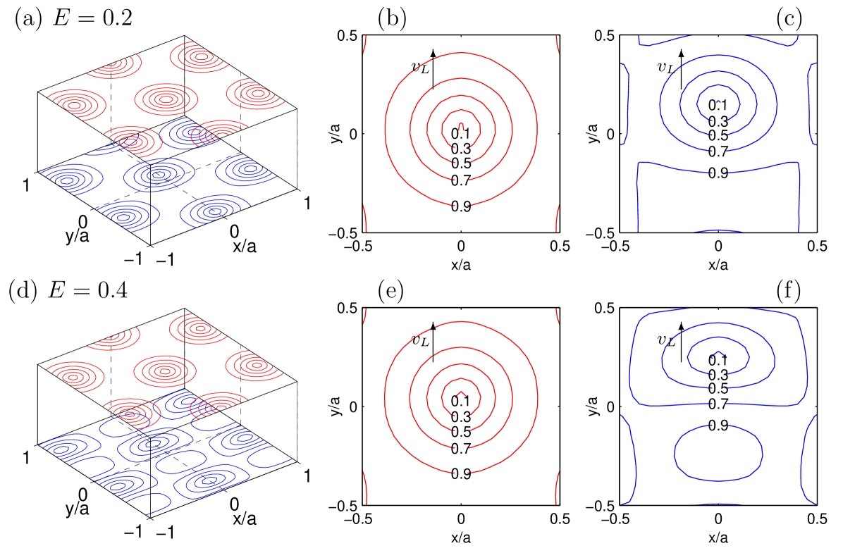
	$\displaystyle{\bm{b}}_{1}=\frac{ieE}{2\pi T}\hat{A}_{1}^{-1}\psi^{\prime}(1/2+\hat{\rho})\bm{b}_{0},$		(32)
	$\displaystyle\hat{A}_{1}=\hat{A}+\psi(1/2+3\hat{\rho})-\psi(1/2+\hat{\rho}).$

The above relation between components of vectors ${\bm{b}_{1}}$ and ${\bm{b}_{0}}$ characterizes splitting of composite vortex into separate constituents. Generally, splitting is present for any non-degenerate multiband superconductor having different diffusivities and coupling constants in the bands. By increasing strength of electric field, distortion of vortex lattice becomes more evident, see Fig. (1).

The moving lattice distortions is induced by the first LL admixture in Eq.(32) which generates a finite net current perpendicular to the vortex velocity. From Eq.(19) we obtain

\displaystyle\sigma_{fl}=\sum_{k}\frac{\langle|\Delta_{k}|^{2}\rangle}{4\pi TeE}\frac{\sigma_{k}}{\rho_{k}}\frac{{\rm Im}(b^{*}_{k0}b_{k1})}{|b_{k0}|^{2}}\left[\psi(1/2+3\rho_{k})-\psi_{k}\right],

(33)

where $\psi_{k}=\psi(1/2+\rho_{k})$ and the average order parameter amplitude is given by $\langle|\Delta_{k}|^{2}\rangle=\sqrt{\pi}|b_{k0}|^{2}L_{H}/x_{0}$ .

III.2 Conductivity correction $\sigma_{st}$ .

To calculate the second term contribution in (6) giving the conductivity correction $\sigma_{st}$ (20) we need to find out how the diffusion coefficients ${\cal D}^{(k)}_{T}$ are modulated by the vortex lattice. For this we determine spectral functions $\hat{g}^{R,A}_{k}$ using the linearised Usadel Eq. (21) supplemented by the normalization condition $(\hat{g}^{R,A}_{k})^{2}=1$ :

		$\displaystyle\hat{g}^{R}_{k}=\left[1+\frac{\|\Delta_{k}\|^{2}}{2(iq_{k}+\varepsilon)^{2}}\right]\tau_{3}+\frac{i\|\Delta_{k}\|\tau_{2}e^{-i\varphi_{k}\tau_{3}}}{iq_{k}+\varepsilon}$		(34)
		$\displaystyle\hat{g}^{A}_{k}=-\left[1+\frac{\|\Delta_{k}\|^{2}}{2(iq_{k}-\varepsilon)^{2}}\right]\tau_{3}+\frac{i\|\Delta_{k}\|\tau_{2}e^{-i\varphi_{k}\tau_{3}}}{iq_{k}-\varepsilon}.$		(35)

Substituting these expressions to the Eq.(15 ) we get

{\cal D}^{(k)}_{T}=2D_{k}\left[1+\frac{|\Delta_{k}|^{2}}{2q_{k}(q_{k}+i\varepsilon)}-\frac{|\Delta_{k}|^{2}}{2(q_{k}+i\varepsilon)^{2}}+c.c.\right]

(36)

Using Eq.(36) we evaluate the conductivity correction (20) as follows

\sigma_{st}=\sum_{k}\frac{\sigma_{k}\langle|\Delta_{k}|^{2}\rangle}{8\pi^{2}T^{2}}\left(\frac{\psi^{\prime}_{k}}{\rho_{k}}+\psi^{\prime\prime}_{k}\right),

(37)

where $\psi^{(n)}_{k}=\psi^{(n)}(1/2+\rho_{k})$ and the partial conductivities are $\sigma_{k}=2e^{2}\nu_{k}D_{k}$ . One can see that the quasiparticle current (37) is given by the superposition of two single-band contributions.

III.3 Slope of the flux-flow resistivity at $H=H_{c2}(T)$ .

We have found that both the conductivity corrections $\sigma_{fl}$ and $\sigma_{st}$ (33,37) are proportional to the average order parameter $\langle|\Delta_{k}|^{2}\rangle$ which should be expressed through the magnetic field. The average gap functions $\langle|\Delta_{k}|^{2}\rangle=\Delta^{2}a^{2}_{k}$ have a common amplitude which have been calculated in the Ref.(SilaevKappa2 )

\Delta=\left(\frac{eT\delta H}{2\beta_{L}}\frac{\sum_{k}\nu_{k}a^{2}_{k}D_{k}\psi^{\prime}_{k}}{\sum_{k}\nu_{k}a^{4}_{k}\sigma_{k}D_{k}\psi^{\prime 2}_{k}\tilde{\kappa}_{k}^{2}}\right)^{1/2},

(38)

where $\delta H=H_{c2}-H$ and $\beta_{L}$ is an Abrikosov parameter equal to $1.16$ for a triangular latticeAbrikosovParameter . The parameters $\tilde{\kappa}_{k}$ which in the single band case characterize the magnetization slope at $H_{c2}(T)$ Maki ; Caroli are given by

\tilde{\kappa}_{k}=\left(\frac{-\psi^{\prime\prime}_{k}}{16\pi\sigma_{k}D_{k}\psi^{\prime 2}_{k}}\right)^{1/2}.

(39)

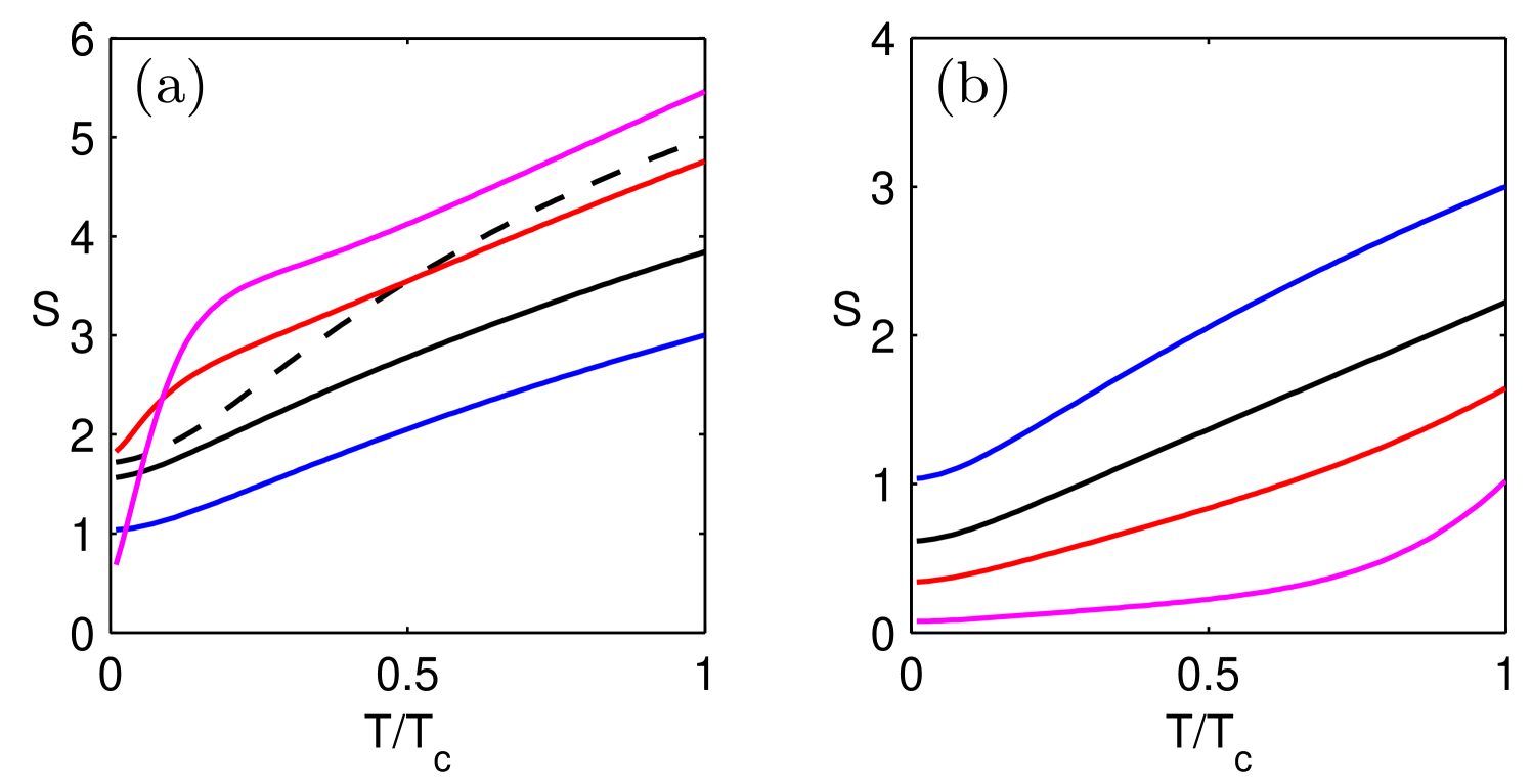
The coefficients $a_{k}$ are determined unambiguously by the Eq.(30) supplemented by a normalization condition $\sum_{k}a_{k}^{2}=1$ so that $a_{k}=|b_{k0}|/\sqrt{\sum_{k}|b_{k0}|^{2}}$ .

Substituting the order parameter amplitude (38) to the expressions for conductivity corrections (19,20) we can find the flux-flow conductivity slope at $H=H_{c2}(T)$ (2) which can by written in the form $S=-(H_{c2}/\sigma_{n})d\sigma_{f}/dH$ . In contrast to the dirty single-band superconductors which are characterized by a universal $S=S(T)$ curve the multiband superconductors have a significant variation of $S$ as a function of the ratio between band diffusivities $D_{1}/D_{2}$ . The sequence of $S(T)$ dependencies for different values of $D_{1}/D_{2}$ are shown in Fig. (2) for the two-band superconductor with pairing constants corresponding to the weak coupling model of MgB₂KoganMgB2 . For the reference the universal single-band curve is shown by the dashed line in Fig.(2)a.

By applying our model at elevated temperatures, we neglect interband impurity scattering assuming that it is much smaller compared to the orbital depairing energy $eD_{k}H_{c2}$ . Due to the same reason we omit scattering at paramagnetic impurities and inelastic electron-phonon relaxationLarkinOvchinnikov which are known to be important near $T_{c}$ but are negligible at lower temperatures.

III.3.1 Limiting values of $S$ at temperatures close to $T_{c}$

Qualitatively the significant deviations of $S(T)$ dependencies from the single-band case can be understood analysing limiting case of $T\to T_{c}$ when the critical field is small so that $\rho_{k}\to 0$ and one can use the asymptotic values of functions $\psi^{\prime}_{k}=\pi^{2}/2$ , $\psi^{\prime\prime}_{k}=-14\zeta(3)$ . In this case the splitting of fractional vortex sub-lattices vanishes. As can be seen from Eqs.(32) to the first order by $\rho_{k}$ we have

{\bm{b}_{1}}=\frac{ieE}{4\pi T}\frac{{\rm Tr}\hat{A}}{\sum_{k}A_{kk}\rho_{k}}{\bm{b}_{0}}.

(40)

This expression means that current-driven fractional vortices in different bands shift by the same amount.

The conductivity corrections are given by

	$\displaystyle\sigma_{fl}=\frac{{\rm Tr}\hat{A}}{\sum_{k}A_{kk}\rho_{k}}\sum_{k}\frac{\sigma_{k}\langle\|\Delta_{k}\|^{2}\rangle}{16T^{2}}$		(41)
	$\displaystyle\sigma_{st}=\sum_{k}\frac{\sigma_{k}\langle\|\Delta_{k}\|^{2}\rangle}{16T^{2}\rho_{k}}.$		(42)

One can see that in contrast to the single band caseThompson these contributions are not equal if the coupling constants are not degenerate $\lambda_{11}\neq\lambda_{22}$ . From Eqs.(38) and (39) we obtain the conductivity slope at $T=T_{c}$

S=S_{c}\frac{\sum_{k}\nu_{k}a_{k}^{2}D_{k}}{2\sum_{k}\nu_{k}a_{k}^{4}}\sum_{k}\frac{\sigma_{k}a_{k}^{2}}{\sigma_{n}}\left(\frac{1}{D_{k}}+\frac{{\rm Tr}\hat{A}}{\sum_{j}A_{jj}D_{j}}\right),

(43)

where $S_{c}=\pi^{4}/(14\zeta(3)\beta_{L})\approx 5$ is the universal value of $S(T=T_{c})$ in the single-component case. Let us consider a two-band system and assume that $\lambda_{11}>\lambda_{22}$ and $\lambda_{12}\ll\lambda_{11}-\lambda_{12}$ , which qualitatively corresponds to the pairing in MgB₂. Then the limiting cases of Eq. (43) are as follows

		$\displaystyle S=\left(1+\frac{A_{22}}{2A_{11}}\right)S_{c},\;\;\;{\rm for}\;\;D_{1}\gg D_{2},$		(44)
		$\displaystyle S=\frac{\lambda_{21}^{2}S_{c}}{2(\lambda_{11}-\lambda_{22})^{2}},\;\;\;{\rm for}\;\;D_{2}\gg D_{1}$		(45)

These expressions are in good agreement with the behaviour of the curves $S(T)$ for MgB₂. As shown in Fig.(2)a, in the limiting case $D_{1}\gg D_{2}$ (the magenta uppermost curve) the value of $S(T_{c})$ is a bit larger that for the single-band case, exactly as described by the Eq.(44) because in this case $A_{22}/A_{11}\approx(\lambda_{11}-\lambda_{22})^{2}/(\lambda_{12}\lambda_{21})$ . In the opposite case $D_{2}\gg D_{1}$ shown in Fig.(2)b (magenta lowermost curve) the value $S(T_{c})\ll S_{c}$ as given by the Eq.(45). Quite amazingly the deviations of $S(T)$ from the single-band case are significant even if one of the diffusivities dominates which means that in the normal state the current flows mostly in one of the bands. At the same time the superconducting corrections $\sigma_{st}$ and $\sigma_{fl}$ are strongly renormalized by multiband effects even in the limiting cases of strong disparity between the diffusivities.

III.3.2 Limiting values of $S$ : the case of decoupled bands

To understand the qualitative features of the flux-flow at high fields it is instructive to consider the case of superconductor with two decoupled bands characterized by different critical temperatures $T_{c1,2}$ . In this case superconductivity at high fields survives only in one of the bands which has the highest critical field $H_{c2}=\max H_{c2}^{(k)}$ . Correspondingly the resistivity slope calculated for this particular band coincides with the universal single-band result Thompson . However even in this case the overall $S$ is still modified by multiband effects. Indeed its definition (2) contains the total normal state conductivity determined by the contribution of all bands, including non-superconducting ones.

Let us consider the analytically tractable low-temperature limit when the single-band critical field is given by $H_{c2}^{(k)}\propto T_{ck}/(eD_{k})$ SingleBandHc2Werthamer ; MakiHc2 ; deGennesHc2 . In this case we obtain $S=S_{0}\sigma_{k}/(\sigma_{1}+\sigma_{2})$ , where $k$ is the component with larger critical field and $S_{0}=2/\beta_{L}\approx 1.72$ is the universal low-temperature limit $S(T=0)$ in the single-component case. It is instructive to consider asymptotic behaviour of $S$ as a function of the diffusivity ratio $d=D_{2}/D_{1}$ . When $d<T_{c2}/T_{c1}$ we have $S=S_{0}\nu_{2}d/(\nu_{1}+\nu_{2}d)$ and $S=S_{0}\nu_{1}/(\nu_{1}+\nu_{2}d)$ in the opposite case when $d>T_{c2}/T_{c1}$ . For non-interacting bands the transition between these regimes is abrupt resulting in the jump on $S(d)$ dependence at $d=T_{c2}/T_{c1}$ . The maximal value of $S$ which can be obtained does not exceed $S_{0}$ .

The origin of a non-monotonic $S(d)$ dependence is determined by the behaviour of $H_{c2}$ in multiband systems. At small $d$ the critical field is determined by the second band which has the smallest diffusivity $H_{c2}=H^{(2)}_{c2}$ . Then with increasing $d$ the superconductivity changes the host band so that $H_{c2}=H^{(1)}_{c2}$ . This transition is an abrupt one for non-interacting bands but a finite interaction makes it the gradual one washing out the cusp singularity. However coupling does not eliminate the non-monotonicity and the asymptotic behaviour of $S(d)$ remains the same as shown in Fig.(4).

IV Small magnetic fields $B\ll H_{c2}$ and low temperatures $T\ll T_{c}$ .

IV.1 General formalism

In dilute vortex configurations at temperatures much below $T_{c}$ the sizeable quasiparticle density exists only inside vortex cores where the superconducting order parameter is suppressed. In this regime the deviations from equilibrium in each band are localized in vortex cores and are significant only at energies much smaller than the bulk energy gaps. Following Kopnin-Gor’kov theoryGorkovKopnin1 , spectral functions $\hat{g}^{R,A}_{k}$ can be parametrized at $\varepsilon=0$ as follows

		$\displaystyle\hat{g}^{R}_{k}$	$\displaystyle=\tau_{3}\cos\theta_{k}+\tau_{2}\sin\theta_{k},$
		$\displaystyle\hat{g}^{A}_{k}$	$\displaystyle=-\tau_{3}\cos\theta_{k}+\tau_{2}\sin\theta_{k}.$

Here we assume that the order parameter vortex phase is removed by gauge transformation. The distribution function can be written in the form

f^{(k)}_{T}=\tilde{f}^{(k)}_{T}v_{L}\partial_{\varepsilon}f_{0}\sin\varphi,

(47)

where $\varphi$ is a polar angle with respect to the vortex center. The amplitude $\tilde{f}^{(k)}_{T}$ is a function of the radial coordinate determined by the following kinetic equation

\left(\frac{d^{2}}{dr^{2}}+\frac{1}{r}\frac{d}{dr}-\frac{1}{r^{2}}\right)\tilde{f}^{(k)}_{T}=\frac{\Delta_{k}\sin\theta_{k}}{D_{k}}\left(2\tilde{f}^{(k)}_{T}-\frac{1}{r}\right)

(48)

with boundary conditions $\tilde{f}^{(k)}_{T}(r=0,\infty)=0$ . The detailed derivation of Eq.(48) is given in the Appendix(A).

The viscous friction force acting on individual moving vortices can be written as ${\bm{F}}_{env}=-\eta{\bm{v}}_{L}$ . The viscosity coefficient $\eta$ can be calculated substituting spectral functions (IV.1) and the distribution function (47) into the expansion (11) and the general expression for the force (10). In this way we obtain

		$\displaystyle\eta=\sum_{k}\pi\hbar\nu_{k}(\alpha_{k}+\gamma_{k}),$		(49)
		$\displaystyle\alpha_{k}=\int_{0}^{\infty}drr\frac{\partial\Delta_{k}}{\partial r}\frac{\partial\sin\theta_{k}}{\partial r},$
		$\displaystyle\gamma_{k}=\int_{0}^{\infty}dr\Delta_{k}\sin\theta_{k}\left(\frac{1}{r}-2\tilde{f}^{(k)}_{T}\right).$

To calculate the gap profiles and spectral functions we use a stationary self-consistency equation written in the form

\Delta_{i}({\bf r})=\sum_{k=1}^{N}\lambda_{ik}\left[\Delta_{k}G_{0}+2\pi T\sum_{n=0}^{\infty}\left(\sin\theta^{M}_{j}-\frac{\Delta_{j}}{\omega_{n}}\right)\right],

(50)

where $G_{0}=({\rm Tr}\hat{\Lambda}-\sqrt{{\rm Tr}\hat{\Lambda}^{2}-4{\rm Det}\hat{\Lambda}})/(2{\rm Det}\hat{\Lambda})-\ln(t)$ and $\hat{\Lambda}=\lambda_{ij}$ is the coupling matrix. In Eq.(50) the summation runs over Matsubara frequencies $\omega_{n}=(2n+1)\pi T$ . The angle $\theta^{M}_{k}$ parametrizes imaginary-frequency Green’s functions similar to Eqs.(IV.1). It is determined by the Usadel equation

\frac{1}{r}\frac{d}{dr}\left(r\frac{d\theta^{M}_{k}}{dr}\right)-\frac{\sin(2\theta^{M}_{k})}{2r^{2}}+\frac{2\Delta_{k}}{D_{k}}\cos\theta^{M}_{k}-\frac{2\omega}{D_{k}}\sin\theta^{M}_{k}=0,

(51)

supplemented by the boundary conditions

		$\displaystyle\theta^{M}_{k}(r=0)=0,$		(52)
		$\displaystyle\theta^{M}_{k}(r=\infty)=\sin^{-1}\left[\Delta_{k}/\left(\Delta_{k}^{2}+\omega^{2}\right)^{1/2}\right].$

One should put $\omega=\omega_{n}$ to obtain solutions at the specific Matsubara frequency. The angle $\theta_{k}$ parametrizing zero-energy spectral functions (IV.1) is given by the same Eqs.(51,52) with $\omega=0$ .

In general the flux-flow conductivity can be expressed through the vortex viscosity (49) as follows GorkovKopnin1

\sigma_{f}=\eta/(B\phi_{0}),

(53)

where $B$ is the average magnetic induction and $\phi_{0}$ is a magnetic flux quantum. Introducing normal-state Drude conductivity $\sigma_{n}=\sum_{k}\sigma_{k}$ , we rewrite flux-flow conductivity (53) in the form

		$\displaystyle\sigma_{f}=\beta\sigma_{n}H_{c2}/B,$		(54)
		$\displaystyle\beta=\frac{1}{2eH_{c2}}\frac{\sum_{k}\nu_{k}(\alpha_{k}+\gamma_{k})}{\sum_{k}\nu_{k}D_{k}}.$		(55)

In Sec.V we analyse parameter $\beta$ for several known multiband compounds superconducting compounds.

IV.2 Exact value of $\beta$ in a single-component case

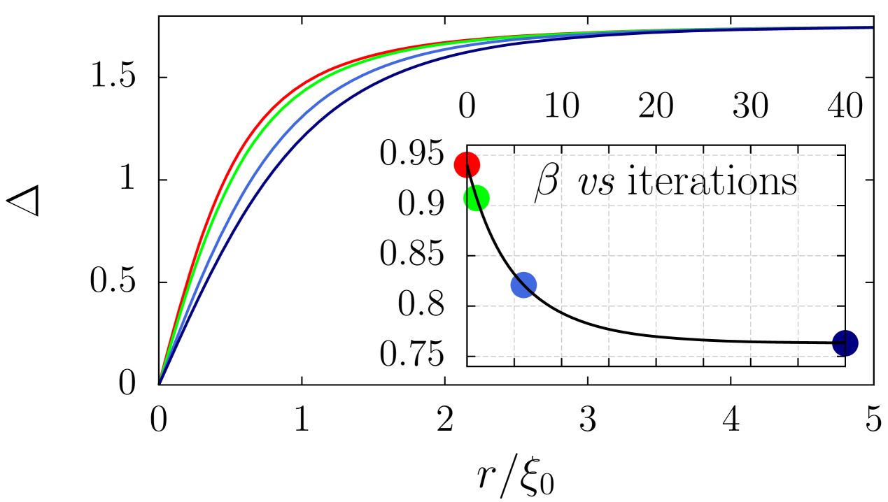
As can be seen from the Eqs.(55) in the single-component case the value of $\beta$ is fixed. Previously the value of $\beta\approx 0.9$ has been reportedGorkovKopnin1 calculated based on the approximate distribution of the order parameter near a vortex watts-tobin . The vortex structure was obtained by a single iteration of the self-consistency Eq.(50) with $N=1$ starting from the Clem-Hao initial guessclem . By performing sufficient iterations of self-consistency equation, one can ascertain that within weak-coupling limit the fully self-consistent vortex structure yields an exact value of $\beta=0.76$ . Fig. 3 demonstrates disparity between initial gap distribution, first iteration and exact gap function together with corresponding values of $\beta$ .

IV.3 Limiting values of $\beta$ : the case of decoupled bands

In multiband superconductors, the flux-flow conductivity behaviour is more involved so that the coefficient $\beta$ can change a lot depending on the ratio of the diffusion constants and pairing potentials in different bands. Below we investigate the maximal accessible values and the asymptotic behaviour of $\beta$ in superconductors with decoupled bands characterized by different critical temperatures $T_{ck}$ . In this case one can adopt single-band results discussed in the previous section IV.2 to obtain

\beta=\beta_{0}\min\left(\frac{D_{k}}{T_{ck}}\right)\frac{\nu_{1}T_{c1}+\nu_{2}T_{c2}}{\nu_{1}D_{1}+\nu_{2}D_{2}},

(56)

where $\beta_{0}\approx 0.76$ is the single-band value. Here we have used the same single-band expression for $H_{c2}=\max H_{c2}^{(k)}$ as in the section (III.3.2).

It is instructive to consider asymptotic behaviour of $\beta$ as a function of the diffusivity ratio $d=D_{2}/D_{1}$ . When $d<T_{c2}/T_{c1}$ we have $\beta=\beta_{0}d(\nu_{2}+\nu_{1}T_{c1}/T_{c2})/(\nu_{1}+\nu_{2}d)$ and $\beta=\beta_{0}(\nu_{1}+\nu_{2}T_{c2}/T_{c1})/(\nu_{1}+\nu_{2}d)$ in the opposite case when $d>T_{c2}/T_{c1}$ . For non-interacting bands the transition between these regimes is abrupt resulting in the sharp maximum $\beta=\beta_{0}$ with a cusp at $d=T_{c2}/T_{c1}$ . The transition results from switching of the superconductivity at $H_{c2}$ between different bands. If there is a finite interband coupling, the cusp in the behaviour of $\beta$ changes to smooth maximum but the maximal value cannot be remarkably enhanced. As a result, parameter $\beta$ in two-band scenario appears to be always limited by its single-band value.

V Examples and comparison with experiments

Having in hand general results we can calculate the flux-flow resistivity in particular multiband superconducting compounds. For that we choose MgB₂ and V₃Si which have been described by the two-band weak coupling modelsKoganMgB2 ; GurevichMgB2 ; KoshelevGolubovMgB2 ; V3Si . Moreover these compounds can have rather large impurity scattering rate to fit the dirty limit conditionsGurevichMgB2 ; KoshelevGolubovMgB2 .

Basically the only input parameters needed to calculate the flux-flow resistivity are the pairing constants which we choose as follows (i) MgB₂ with $\lambda_{11}=0.101$ , $\lambda_{22}=0.045$ , $\lambda_{12}=0.034$ , $\lambda_{21}=0.026$ KoganMgB2 and (ii) V₃Si with $\lambda_{11}=0.26$ , $\lambda_{22}=0.205$ , $\lambda_{12}=\lambda_{21}=0.0088$ V3Si . Note that the parameters of V₃Si correspond to the case of weakly interacting superconducting bands since the interband pairing is much weaker than the intraband one $\lambda_{12}\ll\lambda_{11},\lambda_{22}$ . In that sense it is drastically different from the model of MgB₂ where $\lambda_{12}$ has the same order of magnitude as $\lambda_{11}$ and $\lambda_{22}$ .

For such parameters we apply the results of sections (III.3) and (IV) to find the dependencies $S(d)$ and $\beta(d)$ where $d=D_{2}/D_{1}$ is the ratio of diffusivities in the two bands. The results are shown in Fig.(4). On can see that the dependencies are qualitatively similar for the two sets of pairing constants. The non-monotonicity and asymptotic behaviour of both $S$ and $\beta$ were explained in sections (III.3.2) and (IV.3) using a model of non-interacting bands. As was discussed above the origin of a non-monotonic behaviour is determined by the multiband effects in the near- $H_{c2}$ physics. In that regime increasing the ratio $D_{2}/D_{1}$ one makes the superconductivity to change host band. This affects directly the resistive states at high fields (i.e. the $S$ parameter) but also indirectly the low-field parameter $\beta$ (1) because there the magnetic field dependence is normalized by $H_{c2}$ .

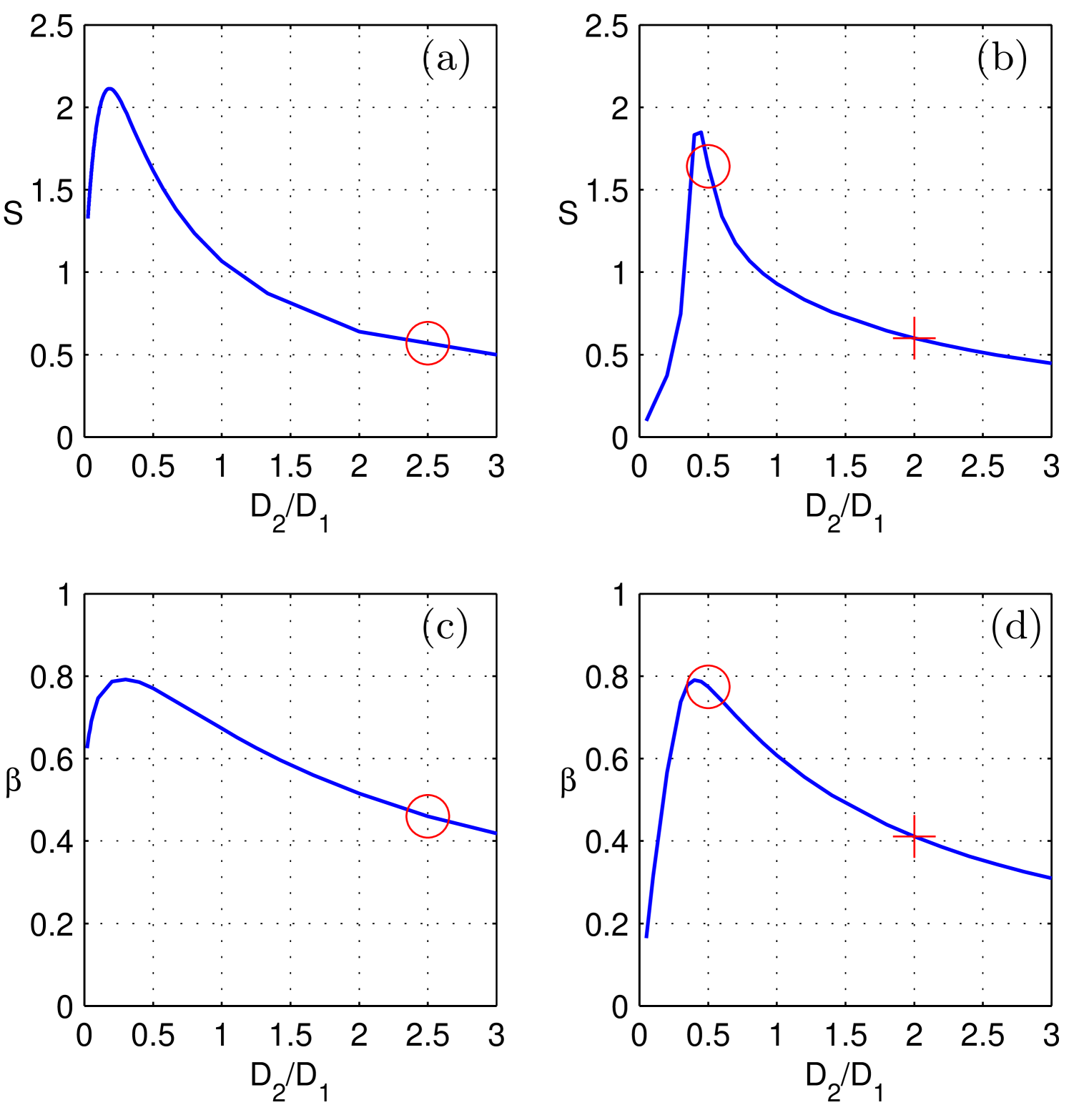
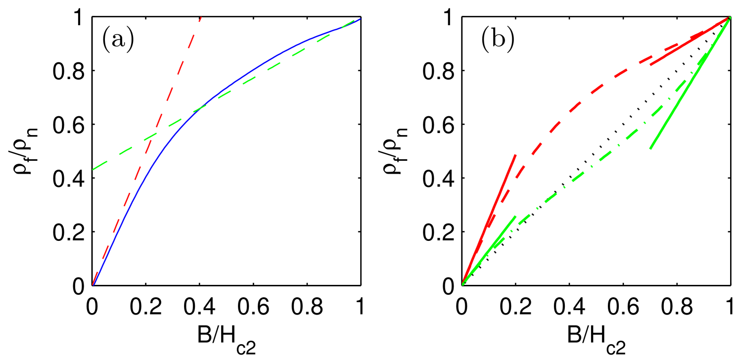
With the help of calculated parameters $S$ and $\beta$ we can reconstruct by extrapolation the flux-flow resistivity curve for the entire range of magnetic field and compare it with the experimental results. In Fig.(5)a we show by dashed lines the slopes that give the best fit of the approximated flux-flow resistivity curve for MgB $2$ at low temperatures $T\ll T_{c}$ , adopted from Ref. (FluxFlowExperimentsMgB2, ). The slopes were calculated using the two-band model for MgB₂ described above. The fitting parameter was the ratio of diffusivities chosen to be $D_{2}/D_{1}=2.5$ marked in the Fig.(4)a,c by open circles.

To understand the possible variations in the shape of the curve $\rho_{f}(B)$ we consider the model corresponding to V₃Si and consider two characteristic values of $D_{2}/D_{1}=2$ and $0.5$ . For such parameters the values of $S$ and $\beta$ are shown by open circles and crosses in the Fig.(4)b,d. One can see that one of these points is in the regime qualitatively similar to the one considered above for MgB₂. Indeed the cubic extrapolation of the $\rho_{f}(B)$ dependence shown by red dashed curve is qualitatively similar to the approximated experimental curve for MgB₂, see Fig.(5). On the other hand, the point $D_{2}/D_{1}=0.5$ belongs to the region where $S>1$ , which results in a different behaviour shown in Fig.(5)b with green color. Experimental data for V₃Si V3Si_2 demonstrates flux-flow resistivity curve between two cases considered, however more measurements are needed to cover whole range of magnetic fields. Note that green curve in Fig. (5)b is quite close to the usual BS linear dependence (black dotted curve) although deflects slightly changing its shape from the concave at small fields to the convex one at large fields. Slightly varying ratio $D_{2}/D_{1}$ around $0.5$ , one can achieve better approach to BS line. At the same time since $\beta$ does not exceed much its single-band limit value $\beta_{0}=0.76$ it is impossible to get a convex curve already at small fields since that would require $\beta>1$ which we did not obtain for the models considered in the present work.

VI Summary

To summarize we have developed theoretical framework to study non-equilibrium processes in multiband superconductors and applied it to calculate flux-flow resistivity of such systems in the dirty limit with high concentration of non-magnetic impurities. We have considered both the regions of high and and low magnetic fields. To calculate the conductivity in the former case we have derived the solution charactering moving vortex lattices which reveals the effect of splitting into sublattices of fractional vortices. The maximal value of the flux-flow resistivity slope $S$ at high fields is shown to be close to the universal single-band limit. At the same time the minimal value can be arbitrary small proportional to the disparity of diffusivities in different bands $S\propto\min(D_{1,2})/\max(D_{1,2})$ .

We calculated the parameter $\beta$ which is inverse slope of flux-flow magneto-resistance curve at low magnetic field. For different models of multiband superconductors we have found that the maximal possible value of $\beta$ is close to the the universal single-band constant $\beta_{0}$ . The approximate value of $\beta_{0}$ was found by Kopnin and Gor’kovGorkovKopnin1 . The exact value calculated in the present work is $\beta_{0}=0.76$ . For large disparity of diffusivities it has the asymptotic behaviour $\beta\propto\min(D_{1,2})/\max(D_{1,2})$ which is similar to that of parameter $S$ .

We demonstrated that multiband superconductors exhibit unconventional generic regime which is characterized by small values of parameters $\beta$ and $S$ and corresponds to the concave flux-flow magnetoresistance curves $\rho_{f}(B)$ . Several recent experimentsFluxFlowExperimentsFeAs1 ; FluxFlowExperimentsFeAs2 ; FluxFlowExperimentsFeAs3 ; FluxFlowExperimentsFeAs4 ; FluxFlowExperimentsFeAs5 ; FluxFlowExperimentsMgB2 confirm that behaviour. For MgB₂ we have obtained a quantitative agreement with experimental results FluxFlowExperimentsMgB2 choosing the ratio of diffusivities in two bands $D_{2}/D_{1}=2.5$ . At the same time we have shown that by varying the parameter $D_{2}/D_{1}$ it is possible to obtain regimes when the curve $\rho_{f}(B)$ is quite close to the single-band Bardeen-Stephen law. Therefore, the suggested theory naturally explains quite diverse experimental data on the flux-flow resistivity in different mutliband superconducting compounds.

VII Acknowlegements

The work was supported by the Estonian Ministry of Education and Research (grant PUTJD141), Goran Gustafsson Foundation and by the Swedish Research Council grant 642-2013-7837.

Appendix A Derivation of kinetic equations and forces acting on the moving vortex line

A.1 General formalism

The quasiclassical GF matrix in band $k$ is defined as

\check{g}_{k}=\left(\begin{array}[]{cc}\hat{g}^{R}_{k}&\hat{g}^{K}_{k}\\ 0&\hat{g}^{A}_{k}\\ \end{array}\right)\;,

(57)

where $g^{K}_{k}$ is the (2 $\times$ 2 matrix) Keldysh component and $\hat{g}^{R(A)}_{k}$ is the retarded (advanced) GF. In a diffusive superconducting wire with band diffusion constants $D_{k}$ the matrix $\check{g}_{k}$ obeys the Usadel equation

\{\tau_{3}\partial_{t},\check{g}_{k}\}_{t}=D_{k}\hat{\partial}_{\bf r}(\check{g}_{k}\circ\hat{\partial}_{\bf r}\check{g}_{k})+[\hat{H}_{k},\check{g}_{k}]_{t}-i[\check{\Sigma}^{ph}_{k},\check{g}_{k}]_{t},

(58)

where $\hat{H}_{k}({\bm{r}},t)=i\hat{\Delta}_{k}$ and $\hat{\Delta}_{k}(t)=|\Delta_{k}|\sigma_{3}\tau_{3}\tau_{1}e^{-i\varphi_{k}\tau_{3}}$ is the gap operator and $\varphi_{k}$ is the gap phase. It is convenient to remove the spin dependence of gap by transformation $\check{g}=\check{U}\check{g}^{new}\check{U}^{+}$ where

\check{U}=\exp\left[i\pi(\sigma_{3}\tau_{3}-\sigma_{0}\tau_{3}-\sigma_{3}\tau_{0})/4\right],

(59)

which leads to

\check{\Delta}^{new}_{k}=\check{U}^{+}\check{\Delta}_{k}\check{U}=i|\Delta_{k}|\tau_{2}e^{-i\varphi_{k}\tau_{3}},

(60)

so that $\hat{H}_{k}({\bm{r}},t)=i\hat{\Delta}_{k}^{new}$ . Note that we use from the beginning the temporal gauge where the scalar potential is zero $\Phi=0$ with and additional constraint that in equilibrium the vector potential is time-independent and satisfies $\nabla\cdot\bm{A}=0$ . Throughout the derivation we assume $k_{B}=\hbar=c=1$ .

The covariant differential superoperator in Eq. (58) is given by

\hat{\partial}_{\bf r}\hat{g}_{k}=\nabla\hat{g}_{k}-ie\left[\tau_{3}{\bm{A}},\hat{g}_{k}\right]_{t}.

Here the commutator operator is defined as $[X,g]_{t}=X(t_{1})g(t_{1},t_{2})-g(t_{1},t_{2})X(t_{2})$ , similarly for anticommutator $\{X,g\}_{t}$ . We also introduce the symbolic product operator $(A\circ B)(t_{1},t_{2})=\int dtA(t_{1},t)B(t,t_{2})$ . Equation (58) is complemented by the normalization condition $(\check{g}_{k}\circ\check{g}_{k})(t_{1},t_{2})=\check{\delta}(t_{1}-t_{2})$ which allows to introduce parametrization of the Keldysh component in terms of the distribution function

	$\displaystyle\hat{g}^{K}_{k}=\hat{g}^{R}_{k}\circ\hat{f}^{(k)}-\hat{f}^{(k)}\circ\hat{g}^{A}_{k},$		(61)
	$\displaystyle\hat{f}^{(k)}=f_{L}^{(k)}\tau_{0}+f_{T}^{(k)}\tau_{3}.$		(62)

Here we will neglect the electron-phonon relaxation given by the last term in the Eq.(58). Such approximation is valid provided the temperature is not too close to $T_{c}$ . In this case the components of the Keldysh-Usadel Eq. (58) read as

		$\displaystyle\{\tau_{3}\partial_{t},\hat{g}^{R(A)}_{k}\}_{t}=D_{k}\hat{\partial}_{\bf r}(\hat{g}^{R(A)}_{k}\circ\hat{\partial}_{\bf r}\hat{g}^{R(A)}_{k})+[\hat{H}_{k},\hat{g}^{R(A)}_{k}]_{t},$
		$\displaystyle\{\tau_{3}\partial_{t},\hat{g}^{K}_{k}\}_{t}=D_{k}\hat{\partial}_{\bf r}(\hat{g}^{R}_{k}\circ\hat{\partial}_{\bf r}\hat{g}^{K}_{k}+\hat{g}^{K}_{k}\circ\hat{\partial}_{\bf r}\hat{g}^{A}_{k})+[\hat{H}_{k},\hat{g}^{K}_{k}]_{t}.$		(63)

To obtain kinetic equation we substitute parametrization (8) to write

	$\displaystyle\hat{\partial}_{\bf r}(\check{g}_{k}\circ\hat{\partial}_{\bf r}\check{g}_{k})^{K}=\hat{\partial}_{\bf r}(\hat{\partial}_{\bf r}\hat{f}^{(k)}-\hat{g}^{R}_{k}\circ\hat{\partial}_{\bf r}\hat{f}^{(k)}\circ\hat{g}^{A}_{k})+$		(64)
	$\displaystyle\hat{g}^{R}_{k}\circ\hat{\partial}_{\bf r}\hat{g}^{R}_{k}\circ\hat{\partial}_{\bf r}\hat{f}^{(k)}-\hat{\partial}_{\bf r}\hat{f}^{(k)}\circ\hat{g}^{A}_{k}\circ\hat{\partial}_{\bf r}\hat{g}^{A}_{k}+$
	$\displaystyle\hat{\partial}_{\bf r}(\hat{g}^{R}_{k}\circ\hat{\partial}_{\bf r}\hat{g}^{R}_{k})\circ\hat{f}^{(k)}-\hat{f}^{(k)}\circ\hat{\partial}_{\bf r}(\hat{g}^{A}_{k}\circ\hat{\partial}_{\bf r}\hat{g}^{A}_{k}).$

To derive this expression we used the associative property of differential superoperator $\hat{\partial}_{\bf r}(g_{1}\circ g_{2})=\hat{\partial}_{\bf r}g_{1}\circ g_{2}+g_{1}\circ\hat{\partial}_{\bf r}g_{2}$ . To get rid of the last two terms we subtract the spectral components of the Eq.(58) to obtain finally the equation

	$\displaystyle\hat{g}^{R}_{k}\circ(\tau_{3}\partial_{t^{\prime}}\hat{f}^{(k)}+\partial_{t_{2}}\hat{f}^{(k)}\tau_{3})-$
	$\displaystyle(\tau_{3}\partial_{t_{1}}\hat{f}^{(k)}+\partial_{t^{\prime}}\hat{f}^{(k)}\tau_{3})\circ\hat{g}^{A}_{k}=$
	$\displaystyle D_{k}\hat{\partial}_{\bf r}(\hat{\partial}_{\bf r}\hat{f}^{(k)}-\hat{g}^{R}_{k}\circ\hat{\partial}_{\bf r}\hat{f}^{(k)}\circ\hat{g}^{A}_{k})+$
	$\displaystyle D_{k}(\hat{g}^{R}_{k}\circ\hat{\partial}_{\bf r}\hat{g}^{R}_{k}\circ\hat{\partial}_{\bf r}\hat{f}^{(k)}-\hat{\partial}_{\bf r}\hat{f}^{(k)}\circ\hat{g}^{A}_{k}\circ\hat{\partial}_{\bf r}\hat{g}^{A}_{k})+$
	$\displaystyle\hat{g}^{R}_{k}\circ[\hat{H}_{k},\hat{f}^{(k)}]_{t}-[\hat{H}_{k},\hat{f}^{(k)}]_{t}\circ\hat{g}^{A}_{k},$		(65)

where $t^{\prime}$ is integration variable.

To proceed we introduce the mixed representation in the time-energy domain as follows $g(t_{1},t_{2})=\int_{-\infty}^{\infty}g(\varepsilon,t)e^{-i\varepsilon(t_{1}-t_{2})}\frac{d\varepsilon}{2\pi}$ , where $t=(t_{1}+t_{2})/2$ . By keeping the first order terms in frequency, we get for Fourier transformations

	$\displaystyle[\hat{H},\hat{g}]_{t}=[\hat{H},\hat{g}]-\frac{i}{2}\{\partial_{t}\hat{H},\partial_{\varepsilon}\hat{g}\},$		(66)
	$\displaystyle[\bm{A}\tau_{3},\hat{g}]_{t}=\bm{A}[\tau_{3},\hat{g}]-\frac{i}{2}\partial_{t}\bm{A}\{\tau_{3},\partial_{\varepsilon}\hat{g}\},$		(67)
	$\displaystyle\hat{\partial}_{\bf r}{\hat{f}}^{(k)}=\nabla\hat{f}^{(k)}+e{\bm{E}}\partial_{\varepsilon}f_{0}\tau_{3},$		(68)

where ${\bm{E}}=-\partial_{t}{\bm{A}}$ is electric field in temporal gauge and $f_{0}=\tanh\varepsilon/(2T)$ is equilibrium distribution. To the first order in frequency and deviation from equilibrium we also have

	$\displaystyle\hat{\partial}_{\bf r}(\hat{\partial}_{\bf r}\hat{f}^{(k)}-\hat{g}^{R}_{k}\circ\hat{\partial}_{\bf r}\hat{f}^{(k)}\circ\hat{g}^{A}_{k})=$
	$\displaystyle\nabla(\nabla f^{(k)}-\hat{g}^{R}_{k}\nabla f^{(k)}\hat{g}^{A}_{k})+e\partial_{\varepsilon}f_{0}\nabla\cdot({\bm{E}}(\tau_{3}-\hat{g}^{R}_{k}\tau_{3}\hat{g}^{A}_{k}))$
	$\displaystyle+ie[{\bm{A}}\tau_{3},\hat{g}^{R}_{k}\nabla\hat{f}^{(k)}\hat{g}^{A}_{k}]+ie^{2}\partial_{\varepsilon}f_{0}({\bm{A}}\cdot{\bm{E}})[\tau_{3},\hat{g}^{R}_{k}\tau_{3}\hat{g}^{A}_{k}].$

The last to terms do not contribute to the kinetic equation since they are traced out.

In the mixed representation the kinetic Eq.(A.1) has the following gauge-invariant form

	$\displaystyle\hat{g}^{R}_{k}\tau_{3}\partial_{t}\hat{f}^{(k)}-\tau_{3}\partial_{t}\hat{f}^{(k)}\hat{g}^{A}_{k}=D_{k}\nabla(\nabla f^{(k)}-\hat{g}^{R}_{k}\nabla f^{(k)}\hat{g}^{A}_{k})+$
	$\displaystyle D_{k}(\hat{g}^{R}_{k}\hat{\partial}_{\bf r}\hat{g}^{R}_{k}\nabla\hat{f}^{(k)}-\nabla\hat{f}^{(k)}\hat{g}^{A}_{k}\hat{\partial}_{\bf r}\hat{g}^{A}_{k})+\hat{g}^{R}_{k}[\hat{H}_{k},\hat{f}^{(k)}]-$
	$\displaystyle[\hat{H}_{k},\hat{f}^{(k)}]\hat{g}^{A}_{k}-i\partial_{\varepsilon}f_{0}(\hat{g}^{R}_{k}\partial_{t}\hat{H}_{k}-\partial_{t}\hat{H}_{k}\hat{g}^{A}_{k})+$		(69)
	$\displaystyle eD_{k}\partial_{\varepsilon}f_{0}\nabla\cdot\left({\bm{E}}(\tau_{3}-\hat{g}^{R}_{k}\tau_{3}\hat{g}^{A}_{k})\right)+$
	$\displaystyle eD_{k}\partial_{\varepsilon}f_{0}{\bm{E}}\cdot(\hat{g}^{R}_{k}\hat{\partial}_{\bf r}\hat{g}^{R}_{k}\tau_{3}-\tau_{3}\hat{g}^{A}_{k}\hat{\partial}_{\bf r}\hat{g}^{A}_{k}),$

where we omit the terms which will be traced out later. The last two terms in Eq. (A.1) are the sources of disequilibrium. Multiplying by $\tau_{3}$ and taking the trace we obtain

		$\displaystyle\nabla({\cal D}_{T}^{(k)}\nabla f_{T}^{(k)})+{\bm{j}}_{e}^{(k)}\cdot\nabla f_{L}^{(k)}+2i{\rm Tr}[(\hat{g}^{R}_{k}+g^{A}_{k})\hat{\Delta}_{k}]f_{T}^{(k)}=$
		$\displaystyle\partial_{\varepsilon}f_{0}{\rm Tr}[\tau_{3}\partial_{t}\hat{\Delta}_{k}(\hat{g}^{R}_{k}+\hat{g}^{A}_{k})]-e\partial_{\varepsilon}f_{0}\nabla\cdot({\cal D}_{T}^{(k)}{\bm{E}}),$		(70)

where the energy dependent diffusion coefficients and the spectral charge currents are

	$\displaystyle{\cal D}_{T}^{(k)}=D_{k}{\rm Tr}(\tau_{0}-\tau_{3}\hat{g}^{R}_{k}\tau_{3}\hat{g}^{A}_{k}),$		(71)
	$\displaystyle{\bm{j}}_{e}^{(k)}=D_{k}{\rm Tr}\;[\tau_{3}(\hat{g}^{R}_{k}\hat{\partial}_{\bf r}\hat{g}^{R}_{k}-\hat{g}^{A}_{k}\hat{\partial}_{\bf r}\hat{g}^{A}_{k})].$		(72)

Analogously taking just the trace of Eq.(A.1) we obtain

		$\displaystyle\nabla({\cal D}_{L}^{(k)}\nabla f_{L}^{(k)})+{\bm{j}}_{e}^{(k)}\cdot\nabla f_{T}^{(k)}+2i{\rm Tr}[\tau_{3}(\hat{g}^{R}_{k}-g^{A}_{k})\hat{\Delta}_{k}]f_{T}^{(k)}=$
		$\displaystyle-\partial_{\varepsilon}f_{0}{\rm Tr}[\partial_{t}\hat{\Delta}_{k}(\hat{g}^{R}_{k}-\hat{g}^{A}_{k})]-e\partial_{\varepsilon}f_{0}\left({\bm{j}}_{e}^{(k)}\cdot{\bm{E}}\right),$		(73)

where ${\cal D}_{L}^{(k)}=D_{k}{\rm Tr}(\tau_{0}-\hat{g}^{R}_{k}\hat{g}^{A}_{k})$ . Here we took into account that ${\rm Tr}(\hat{g}^{R}_{k}\tau_{3}\hat{g}^{A}_{k})=0$ because of the relation $\hat{g}^{A}_{k}=-\tau_{3}\hat{g}^{R+}_{k}\tau_{3}$ and the general form of the equilibrium spectral function $\hat{g}^{R}_{k}=g_{3}^{(k)}\tau_{3}+g_{2}^{(k)}\tau_{2}e^{-i\varphi_{k}\tau_{3}}$ .

A.2 The low temperature limit $T\ll T_{c}$ .

At low temperatures the deviations from equilibrium are localized in the vortex core and are significant only at small energies. Therefore following Kopnin-Gor’kov theory we can use the spectral functions $\hat{g}^{R,A}_{k}$ calculated at $\varepsilon=0$ when it is possible to use $\theta$ parametrization in each band

	$\displaystyle\hat{g}^{R}_{k}=\tau_{3}\cos\theta_{k}+\tau_{2}e^{-i\tau_{3}\varphi_{k}}\sin\theta_{k},$		(74)
	$\displaystyle\hat{g}^{A}_{k}=-\tau_{3}\hat{g}^{R+}_{k}\tau_{3}.$

In this case we can simplify kinetic equation with the help of the following identities ${\cal D}^{(k)}_{T}=4D_{k}$ and

	$\displaystyle 2i{\rm Tr}[(\hat{g}^{R}_{k}+\hat{g}^{A}_{k})\hat{\Delta}_{k}]=-8\|\Delta_{k}\|\sin\theta_{k},$		(75)
	$\displaystyle{\rm Tr}[\tau_{3}\partial_{t}\hat{\Delta}_{k}(\hat{g}^{R}_{k}+\hat{g}^{A}_{k})]=4({\bm{v}}_{L}\cdot\nabla\varphi_{k})\|\Delta_{k}\|\sin\theta_{k},$		(76)

where we took into account that for the vortex moving with constant velocity $\partial_{t}\Delta_{k}=-{\bm{v}}_{L}\cdot\nabla\Delta_{k}$ . Hence the kinetic equation becomes

D_{k}\nabla^{2}f^{(k)}_{T}=\left[2f^{(k)}_{T}+\partial_{\varepsilon}f_{0}({\bm{v}}_{L}\nabla\varphi_{k})\right]|\Delta_{k}|\sin\theta_{k}.

(77)

To calculate the force ${\bm{F}}_{env}$ (9) we use the expansion (11) substituting there the spectral functions in the form (74) to obtain

	$\displaystyle{\rm Tr}(\hat{g}^{nst}_{k}\hat{\partial}_{\bm{r}}\hat{\Delta}_{k})=-2\partial_{\varepsilon}f_{0}[({\bm{v}}_{L}\nabla\sin\theta_{k})]\nabla\|\Delta_{k}\|$		(78)
	$\displaystyle-2\sin\theta_{k}\|\Delta_{k}\|\left[2f^{(k)}_{T}+\partial_{\varepsilon}f_{0}({\bm{v}}_{L}\nabla\varphi_{k})\right]\nabla\varphi_{k}.$

For small magnetic fields $B\ll H_{c2}$ the last term in Eq.(9) can be neglected so that the force is given by

	$\displaystyle{\bm{F}}_{env}=-\sum_{k}\frac{\nu_{k}}{2}\int d^{2}{\bm{r}}d\varepsilon\Big{\{}\partial_{\varepsilon}f_{0}\nabla\|\Delta_{k}\|({\bm{v}}_{L}\nabla\sin\theta_{k})+$
	$\displaystyle\|\Delta_{k}\|\sin\theta_{k}\left[2f^{(k)}_{T}+\partial_{\varepsilon}f_{0}({\bm{v}}_{L}\nabla\varphi_{k})\right]\nabla\varphi_{k}\Big{\}}.$		(79)

We can simplify equations further taking into account common phase $\varphi_{1,2}=\varphi$ so that $({\bm{v}}_{L}\nabla\varphi)=-v_{L}\sin\varphi/r$ and $({\bm{v}}_{L}\nabla|\Delta_{k}|)=v_{L}\cos\varphi\partial_{r}|\Delta_{k}|$ . By factorizing the angular dependence of the distribution function $f^{(k)}_{T}=\tilde{f}^{(k)}_{T}v_{L}\partial_{\varepsilon}f_{0}\sin\varphi$ , the force becomes ${\bm{F}}_{env}=-\eta{\bm{v}}_{L}$ where the viscosity coefficient is given by (49).

References

(1) T. Okada, H. Takahashi, Y. Imai, K. Kitagawa, K. Matsubayashi, Y. Uwatoko, and A. Maeda, Physica C 484, 27 (2013).
(2) T. Okada, H. Takahashi, Y. Imai, K. Kitagawa, K. Matsubayashi, Y. Uwatoko, and A. Maeda, Phys. Rev. B 86, 064516 (2012).
(3) T. Okada, Y. Imai, H. Takahashi, M. Nakajima, A. Iyo, H. Eisaki, and A. Maeda, Physica C 504, 24 (2014).
(4) H. Takahashi, T. Okada, Y. Imai, K. Kitagawa, K. Matsubayashi, Y. Uwatoko, and A. Maeda, Phys. Rev. B 86, 144525 (2012).
(5) T. Okada, F. Nabeshima, H. Takahashi, Y. Imai, and A. Maeda, Phys. Rev. B 91, 054510 (2015).
(6) A. Shibata, M. Matsumoto, K. Izawa, Y. Matsuda, S. Lee, and S. Tajima Phys. Rev. B 68, 060501(R) (2003).
(7) Y.B. Kim, C.F. Hempstead, and A. R. Strnad, Phys. Rev., 139, Al163 (1965).
(8) J. Bardeen and M.J. Stephen, Phys. Rev., 140, A1197 (1965).
(9) L.P. Gor’kov and N.B. Kopnin, Zh. Eksp. Teor. Fiz. 65, 396 (July 1973) [ Sov. Phys. JETP, 38, 195 (1974)].
(10) L.P. Gor’kov and N.B. Kopnin, Zh. Eksp. Teor. Fiz. 64 356 (1973) [Sov. Phys. JETP, 37, 183 (1973)].
(11) C. Caroli and K. Maki, Phys. Rev. 164, 591 (1967).
(12) R.S. Thompson, Phys. Rev. B 1, 327 (1970).
(13) H. Tokoyama, H. Ebisawa, Prog. Theor. Phys. 44, 1450 (1970).
(14) A. Schmid, Phys. kondens. materie 5, 302 (1966).
(15) N. Ya. Fogel, Zh. Eksp. Teor. Fiz. 63 1371 (1972), [Sov. Phys. JETP, 36, 725 (1973)].
(16) Yu.N. Ovchinnikov, Zh. Eksp. Teor. Fiz. 65 290 (1973) [Sov. Phys. JETP, 38, 143 (1974)].
(17) R. Meier-Hirmer, M.D. Maloney, and W. Gey, Z. Physik B, 23, 139 (1976).
(18) A. I. Larkin, and Yu. N. Ovchinnikov in Modern Problems in Condensed Matter Sciences: Nonequilibrium Superconductivity eds. D.N. Langenberg and A.I. Larkin, p. 493, Elsevier (1986)
(19) E. Babaev, Phys. Rev. Lett. 89, 067001 (2002).
(20) E. Smorgrav, J. Smiseth, E. Babaev, and A. Sudbo, Phys. Rev. Lett. 94, 096401 (2005).
(21) L. F. Chibotaru, V. H. Dao, and A. Ceulemans, EPL 78, 47001 (2007).
(22) M. A. Silaev, Phys. Rev. B 83, 144519 (2011).
(23) S. Z. Lin and L. N. Bulaevskii, Phys. Rev. Lett. 110, 087003 (2013).
(24) M. Silaev, Phys. Rev. B 93, 214509 (2016).
(25) W.H. Kleiner, L.M. Roth, S.H. Autler, Phys. Rev. A133 1226 (1964).
(26) K. Maki, Physics, 1, 21 (1964).
(27) C. Caroli, M. Cyrot, P.G. de Gennes, Solid State Comm. 4 17 (1966).
(28) A. Gurevich, Phys. Rev. B 67, 184515 (2003).
(29) A. A. Golubov and A. E. Koshelev, Phys. Rev. B 68, 104503 (2003).
(30) F. Hunte, J. Jaroszynski, A. Gurevich, D. C. Larbalestier, R. Jin, A. S. Sefat, M. A. McGuire, B. C. Sales, D. K. Christen, D. Mandrus, Nature 453, 903 (2008).
(31) E.A. Yelland, J.R. Cooper, A. Carrington, N.E. Hussey, P.J. Meeson, S. Lee, A. Yamamoto, and S. Tajima, Phys. Rev. Lett. 88, 217002 (2002).
(32) A.V. Sologubenko, J.Jun, S.M. Kazakov, J. Karpinski, and H.R. Ott, Phys. Rev. B 66, 014504 (2002).
(33) M.R. Eskildsen, M. Kugler, S. Tanaka, J. Jun, S.M. Kazakov, J. Karpinski, and O. Fischer, Phys. Rev. Lett. 89, 187003 (2002).
(34) V. Braccini, A. Gurevich, J. E. Giencke, M. C. Jewell, C. B. Eom, D. C. Larbalestier, A. Pogrebnyakov, Y. Cui, B. T. Liu, Y. F. Hu, J. M. Redwing, Qi Li, X. X. Xi, R. K. Singh, R. Gandikota, J. Kim, B. Wilkens, N. Newman, J. Rowell, B. Moeckly, V. Ferrando, C. Tarantini, D. Marre, M. Putti, C. Ferdeghini, R. Vaglio, E. Haanappel, Phys. Rev. B 71, 012504 (2005).
(35) V. Ferrando, P. Manfrinetti, D. Marre, M. Putti, I. Sheikin, C. Tarantini, C. Ferdeghini, Phys. Rev. B 68, 094517 (2003).
(36) F. Bouquet, Y. Wang, I. Sheikin, P. Toulemonde, M. Eisterer, H.W. Weber, S. Lee, S. Tajima, A. Junod, Physica C 385, 192 (2003).
(37) A. Gurevich, S. Patnaik, V. Braccini, K. H. Kim, C. Mielke, X. Song, L. D. Cooley, S. D. Bu, D. M. Kim, J. H. Choi, L. J. Belenky, J. Giencke, M. K. Lee, W. Tian, X. Q. Pan, A. Siri, E. E. Hellstrom, C. B. Eom, D. C. Larbalestier, Supercond. Sci. Technol. 17, 278 (2004).
(38) N. Kopnin, Theory of Nonequilibrium Superconductivity, Oxford University Press, 2001
(39) G. Schön in Modern Problems in Condensed Matter Sciences: Nonequilibrium Superconductivity eds. D.N. Langenberg and A.I. Larkin, p. 589-640, Elsevier (1986)
(40) V. G. Kogan, C. Martin, and R. Prozorov Phys. Rev. B 80, 014507 (2009).
(41) N.R. Werthamer, E. Helfand, and P.C. Hohenberg, Phys. Rev. 147, 288 (1966).
(42) K. Maki, Phys. Rev. 148, 362 (1966).
(43) P.G. De Gennes, Phys. Cond. Mater. 3, 79 (1964).
(44) R. J. Watts-Tobin and G. M. Waterworth in Low temperature Physics-LT 13: Superconductivity eds. K.D. Timmerbaus, W. J. O’Sullivan and E. F. Hammel, p. 37-41, Springer (1974).
(45) J. R. Clem, J. Low Temp. Phys. 18, 427 (1975).
(46) A. E. Koshelev and A. A. Golubov, Phys. Rev. Lett. 90, 177002 (2003).
(47) Yu. A. Nefyodov, A. M. Shuvaev and M. R. Trunin, Europhys. Lett., 72, 638 (2005).
(48) A. A. Gapud, S. Moraes, R. P. Khadka, P. Favreau, C. Henderson, P. C. Canfield, V. G. Kogan, A. P. Reyes, L. L. Lumata, D. K. Christen, J. R. Thompson, Phys. Rev. B 80, 134524 (2009).