Warm inflationary universe model in light of Planck 2015 results
Abstract
In the present work we show that warm chaotic inflation characterized by a simple self-interaction potential for the inflaton, excluded by current data in standard cold inflation, and by an inflaton decay rate proportional to the temperature, is in agreement with the latest Planck data. The parameters of the model are constrained, and our results show that the model predicts a negligible tensor-to-scalar ratio in the strong dissipative regime, while in the weak dissipative regime the tensor-to-scalar ratio can be large enough to be observed.
pacs:
98.80.CqI Introduction
The inflationary universe has become one of the central paradigms in modern cosmology. This is due to the fact that many long-standing problems of the Big Bang model, such as the horizon, flatness, homogeneity and monopole problems, find a natural explanation in the framework of the inflationary universe R1 ; R106 ; R103 ; R104 ; R105 ; Linde:1983gd . However, the essential feature of inflation is that it generates a mechanism to explain the Large-Scale Structure (LSS) of the universe R2 ; R202 ; R203 ; R204 ; R205 and provides a causal interpretation of the origin of the anisotropies observed in the Cosmic Microwave Background (CMB) radiationastro ; astro2 ; astro202 ; Hinshaw:2012aka ; Ade:2013zuv ; Ade:2013uln , since primordial density perturbations may be produced from quantum fluctuations during the inflationary era.
The original “old inflation” scenario assumed the inflaton was trapped in a metastable false vacuum and had to exit to the true vacuum via a first-order transition R1 ; R106 . However, the exit could occur neither gracefully nor completely. The revised version of inflation was proposed by A. Linde R103 ; R104 , and A. Albrecht and J. Steinhardt R105 in 1982 referred as “new inflation”. However, these scenarios suffer from theoretical problems about the duration of inflation and initial conditions. In 1983, A. Linde considered the case that the initial conditions for scalar field driving inflation may be chaotic, which is called “chaotic inflation” Linde:1983gd . This inflation model can solve the remaining problems, where the potential was chosen to be cuadratic or quartic form, i.e. or , terms that are always present in the scalar potential of the Higgs sector in all renormalizable gauge field theories pich in which the gauge symmetry is spontaneously broken via the Englert-Brout-Higgs mechanism higgs . Such models are interesting for their simplicity, and has become one of the most favored, because they predict a significant amount of tensor perturbations due to the inflaton field gets across the trans-Planckian distance during inflation Lyth:1996im . After that, many kinds of inflationary scenarios have been proposed, related to supersymmetry (SUSY) theory, brane world, string theory, etc. (for review, see Lyth:1998xn ; Riotto:2002yw ; Bassett:2005xm ; Baumann:2014nda ).
On the other hand, with respect to the dynamical mechanisms of inflation, the warm inflation scenario, as opposed to the standard cold inflation, has the attractive feature that it avoids the reheating period at the end of the accelerated expansion warm . During the evolution of warm inflation dissipative effects are important, and radiation production takes place at the same time as the expansion of the universe. The dissipative effects arise from a friction term which accounts for the processes of the scalar field dissipating into a thermal bath. In further relation to these dissipative effects, the dissipative coefficient is a fundamental quantity, which has been computed from first principles in the context of supersymmetry. In particular, in Ref.26 , a supersymmetric model containing three superfields , , and has been studied, with a superpotential , where the scalar components of the superfields are , , and respectively. For a scalar field with multiplets of heavy and light fields, and different decay mechanisms, it is possible to obtain several expressions for the dissipative coefficient , see e.g., 26 ; 28 ; 2802 ; Zhang:2009ge ; BasteroGil:2011xd ; BasteroGil:2012cm .
Following Refs.Zhang:2009ge ; BasteroGil:2011xd , a general parametrization of the dissipative coefficient can be written as
| (1) |
where the parameter is related with the dissipative microscopic dynamics and the exponent is an integer. This expression for the dissipative coefficient includes different cases studied in the literature, depending of the values of (see Refs. Zhang:2009ge ; BasteroGil:2011xd ). Specifically, for the value , i.e., , the parameter corresponds to , where a generic supersymmetric model with chiral superfields , , and has been considered. This case corresponds to a low temperature regime, when the mass of the catalyst field is larger than the temperature BasteroGil:2012cm . On the other hand, , i.e., corresponds to a high temperature regime, where the thermal corrections to the catalyst field mass start to be important, where 26 . For , the dissipative coefficient represents an exponentially decaying propagator in the high temperature regime. Finally, For , i.e., , agrees with the non-SUSY case 28 ; PRD . Additionally, thermal fluctuations during the inflationary scenario may play a fundamental role in producing the primordial fluctuations 62526 ; 1126 . During the warm inflationary scenario the density perturbations arise from thermal fluctuations of the inflaton and dominate over the quantum ones. In this form, an essential condition for warm inflation to occur is the existence of a radiation component with temperature , since the thermal and quantum fluctuations are proportional to and , respectivelywarm ; 62526 ; 1126 . When the universe heats up and becomes radiation dominated, inflation ends and the universe smoothly enters in the radiation Big-Bang phasewarm . For a comprehensive review of warm inflation, see Ref. Berera:2008ar .
Upon comparison to the current cosmological and astronomical observations, specially those related with the CMB temperature anisotropies, it is possible to constrain the inflationary models. In particular, the constraints in the plane give us the predictions of a number of representative inflationary potentials. Recently, the Planck collaboration has published new data of enhanced precision of the CMB anisotropies Ade:2015lrj . Here, the Planck full mission data has improved the upper bound on the tensor-to-scalar ratio ( CL) which is similar to obtained from Ade:2013uln , in which ( CL). In particular, the model, which predicts a large value of the tensor-to-scalar ratio , lies well outside of the joint CL region in the , so it is ruled out by the data. This result confirms previous findings from e.g., Hinshaw et al. Hinshaw:2012aka in which this model is well outside the CL for the WMAP 9-year data and is further excluded by CMB data at smaller scales.
In this way, the goal of the present work is to study the possibility that the model can be rescued in the warm inflation scenario and be able to agree with the latest observational data. In order to achieve this, we consider an inflaton decay rate proportional to the temperature, which has been computed in the context of a high temperature supersymmetric model 26 . We stress that, in previous works (see Ref.BasteroGil:2012cm ), the authors have also studied the quartic potential in the framework of warm inflation. However, our work is different in two ways. First, contrary to the standard cold inflation where the dynamics is determined only by the inflaton potential, in warm inflation also the dissipative coefficient plays an important role, and here we have considered an expression for it not studied in the previous works. Furthermore, in none of these papers the authors used the contour plots in the and plane to constrain the parameters of the model they studied. On the contrary, in our work here we have used the latest data from Planck, not available at that time, to put bounds on the parameters of the model we have considered.
The outline of the paper is as follows: The next section presents a short review of the basics of warm inflation scenario. In Sect. III we study the dynamics of warm inflation for our quartic potential, in the weak and strong dissipative regimes; specifically, we obtain analytical expressions for the slow-roll parameters and the dissipative coefficient. Immediately, we compute the cosmological perturbations in both dissipative regimes, obtaining expressions for the inflationary observables such as the scalar power spectrum, the scalar spectral index, and the tensor-to-scalar ratio. Finally, Sect.IV summarizes our results and exhibits our conclusions. We choose units so that .
II Basics of warm inflation scenario
II.1 Background evolution
We start by considering a spatially flat Friedmann-Robertson-Walker (FRW) universe containing a self-interacting inflaton scalar field with energy density and pressure given by and , respectively, and a radiation field with energy density . The corresponding Friedmann equations reads
| (2) |
where is the reduced Planck mass.
The dynamics of and is described by the equations warm
| (3) |
and
| (4) |
where the dissipative coefficient produces the decay of the scalar field into radiation. Recall that this decay rate can be assumed to be a function of the temperature of the thermal bath , or a function of the scalar field , or a function of or simply a constantwarm .
During warm inflation, the energy density related to the scalar field predominates over the energy density of the radiation field, i.e., warm ; 62526 ; 6252602 ; 6252603 ; 6252604 , but even if small when compared to the inflaton energy density it can be larger than the expansion rate with . Assuming thermalization, this translates roughly into , which is the condition for warm inflation to occur.
When , , and are slowly varying, which is a good approximation during inflation, the production of radiation becomes quasi-stable, i.e., and , see Refs.warm ; 62526 ; 6252602 ; 6252603 ; 6252604 . Then, the equations of motion reduce to
| (5) |
where denotes differentiation with respect to inflaton, and
| (6) |
where is the dissipative ratio defined as
| (7) |
In warm inflation, we can distinguish between two possible scenarios, namely the weak and strong dissipative regimes, defined as and , respectively. In the weak dissipative regime, the Hubble damping is still the dominant term, however, in the strong dissipative regime, the dissipative coefficient controls the damped evolution of the inflaton field.
If we consider thermalization, then the energy density of the radiation field could be written as , where the constant . Here, represents the number of relativistic degrees of freedom. In the Minimal Supersymmetric Standard Model (MSSM), and 62526 . Combining Eqs.(5) and (6) with , the temperature of the thermal bath becomes
| (8) |
On the other hand, the consistency conditions for the approximations to hold imply that a set of slow-roll conditions must be satisfied for a prolonged period of inflation to take place. For warm inflation, the slow-roll parameters are 26 ; 62526
| (9) |
When one these conditions is not longer satisfied, either the motion of the inflaton is no longer overdamped and slow-roll ends, or the radiation becomes comparable to the inflaton energy density. In this way, inflation ends when one of these parameters become the order of .
From first principles in quantum field theory, the dissipative coefficient has been computed. As we have seen in the introduction, the parametrization given by Eq.(1) includes different cases, depending of the values of . Concretely , for , for which , the parameter agrees with , where a generic supersymmetric model with chiral superfields , and , has been considered. In particular, this inflation ratio decay has been studied extensively in the literature BasteroGil:2012cm ; Herrera:2015aja , including the quartic potential Berera:2008ar . For the special case , the dissipative coefficient is related with the high temperature supersymmetry (SUSY) case 26 . Finally, for the cases and , represents an exponentially decaying propagator in the high temperature SUSY model and the non-SUSY case, respectively28 ; PRD .
II.2 Perturbations
In the warm inflation scenario, a thermalized radiation component is present with , then the inflaton fluctuations are predominantly thermal instead quantum. In this way, following 62526 ; 1126 ; Berera:2008ar , the amplitude of the power spectrum of the curvature perturbation is given by
| (11) |
where the normalization has been chosen in order to recover the standard cold inflation result when and .
Regarding to tensor perturbations, these do not couple to the thermal background, so gravitational waves are only generated by quantum fluctuations, as in standard inflation Taylor:2000ze . However, the tensor-to-scalar ratio is modified with respect to standard cold inflation, yielding Berera:2008ar
| (13) |
We can see that warm inflation predicts a tensor-to-scalar ratio suppressed by a factor compared with standard cold inflation.
When a specific form of the scalar potential and the dissipative coefficient are considered, it is possible to study the background evolution under the slow-roll regime and the primordial perturbations in order to test the viability of warm inflation. In the following we will study how an inflaton decay rate proportional to the temperature, corresponding to the case , influences the inflationary dynamics for the quartic potential. We will restrict ourselves to the weak and strong dissipation regimes.
III Dynamics of warm inflation
Although inflation is widely accepted as the standard paradigm for the early universe, it is not a theory yet as we don’t know how to answer the question that naturally arises, ”what is the inflaton and what is its potential?”. After the recent discovery of the Higgs boson at CERN experiments , which showed that elementary scalars exist in nature, the most natural and simplest thing to assume is that inflation is driven by the Higgs boson (in the standard model or in some extension of it). Unfortunately it is well known that the quartic potential, which is the simplest Higgs potential provided by particle physics in renormalizable theories, has been excluded by current data kallosh since it predicts too many gravity waves. Although the presence of a non-minimal coupling can make the quartic potential viable shafi , warm inflation provides another solution that is simpler and at the same time, as we have already mentioned, avoids the discussion about reheating. If we look at the expressions for the observables in the framework of warm inflation, we see that the key ingredient that can in principle reduce the tensor-to-scalar ratio, and bring the predictions of the model inside the region allowed by observational data, is the suppression factors and . And this is exactly what happens indeed as we will show in the discussion to follow.
Warm inflation with a quartic potential for the inflaton has also been studied in BasteroGil:2011xd ; papers . However there are some differences, as in these works the authors have used another expression for the dissipative coefficient, they have not derived the allowed range for the parameters of the model they studied, and finally in our work we have used the most recent data available today.
III.1 The weak dissipative regime
Considering our model evolves in agreement with the weak dissipative regime, where , and that under the slow-roll approximation the Friedmann and the Klein-Gordon equations take the standard form, the temperature of the radiation field assuming an inflaton potential of the form and an inflaton decay rate , becomes
| (14) |
and the Hubble parameter is given by
| (15) |
In this way, for the weak regime, the slow-roll parameters become
| (16) |
It is easy to see that the end of inflation is determined by the condition , where the scalar field takes the value .
By the other hand, the number of -folds is given by the standard formula
| (17) |
where we have assumed that .
In the following, we will study the scalar and tensor perturbations. In the weak dissipative regime, the amplitude of the power spectrum (11) becomes
| (18) |
By using Eqs.(14), (15), and (17), it may we written in terms in the number of -folds as
| (19) |
The power spectrum constraint Ade:2013uln ; Ade:2015lrj determines the dimensionless coupling in terms of and , while the scalar spectral index (12) turns out to be
| (20) |
which may be expressed in terms of the number of the -folds, obtaining
| (21) |
while the tensor-to-scalar ratio (13) becomes
| (22) |
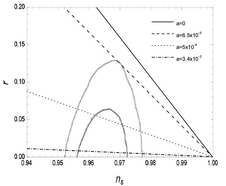
so eventually we can obtain as a function of . Using Eqs.(19), (21), and (22), the relation is given by
| (23) |
In figure 1, the relation is shown for several values of . In the same plot we also show the curve for standard inflation () as well as the contours allowed by the Planck latest data. When decreases the curve is shifted upwards and finally lies outside the allowed contours. This induces a lower bound on . On the other hand, when increases the curve is shifted downwards, but also increases and eventually the condition for being in the weak dissipative regime is violated. This induces an upper bound on , which is found to be . This implies that the Eq.(19), evaluated when the cosmological scales cross the Hubble horizon during inflation at -folds, gives us the constraint on determined by . It is interesting to note that this result is in agreement with the value obtained for in the standard cold inflation using the COBE normalization Liddle:2000cg , given by .
III.2 The strong dissipative regime
Considering our model evolves in agreement with the strong dissipative regime, where , under the slow-roll approximation, the temperature of the radiation field becomes
| (24) |
and the Hubble parameter is given by Eq.(15) In this way, for the strong regime, the slow-roll parameters become
| (25) |
For the strong regime, inflation ends when one of these slow-roll parameters becomes the order of . In this case, the end of inflation is determined by the condition , where the inflaton takes the value .
By the other hand, the number of -folds is given by
| (26) |
where we have assumed that .
Now, the amplitude of the power spectrum (11) becomes
| (27) |
Similarly to weak regime, the amplitude of the power spectrum may we written in terms of the number of -folds. Using Eqs.(15), (24), and (26), we have that
| (28) |
In this case, the power spectrum does not depend on and then the constraint Ade:2013uln ; Ade:2015lrj determines the inflaton self-interaction coupling .
For this regime, the scalar spectral index (12) turns out to be
| (29) |
which expressed in terms of the number of the -folds yields
| (30) |
Finally, for the tensor-to-scalar ratio (13) we have that
| (31) |
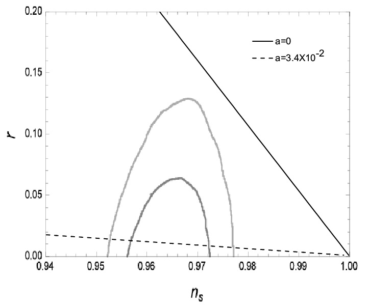
which may be expressed as function of . Using Eqs.(28), (30), and (31), the relation is given by
| (32) |
In figure 2, the relation is shown for two different values of . In the same plot, as in the weak regime, we also show the curve for standard cold inflation () as well as the contours allowed by the latest Planck data. When decreases the curve is shifted upwards, but also decreases and eventually the condition for being in the strong dissipative regime is violated. This induces a lower bound on . By the other hand, when increases the curve is shifted downwards, but also increases and the condition for being in the strong dissipative regime is always satisfied. This implies that there is only a lower bound for found by the requirement of staying in the strong dissipative regime, and given by . Finally, the Eq.(28), evaluated at -folds, gives us the constraint on , determined by . This value is almost the same order that obtained for in the standard cold inflation.
IV Conclusions
In the present work we have studied warm inflation with a quartic inflaton potential and an inflaton decay rate proportional to the temperature, namely . Warm inflation consists an alternative to the standard cold inflation, during which radiation is neglected and which requires two steps, a slow-roll phase followed by a reheating phase, about which very little is known. On the contrary, in warm inflation, which has the attractive feature that avoids reheating, radiation is also taken into account and it is coupled to the inflaton leading to testable predictions different than the predictions of standard inflation even in the weak dissipative regime. The model we have considered is characterized by two parameters, namely the dimensionless couplings and . We have used the latest Planck data to constrain the parameters of the model, and the results we have obtained are shown in the figures 1 and 2 for the case of weak and strong dissipative regime respectively. In the weak regime first, where , the background equations look the same as in standard inflation, however the tensor-to-scalar ratio is suppressed by the factor , which must always be larger than one in warm inflation. The power spectrum constraint determines in terms of , and then the tensor-to-scalar ratio as a function of the scalar index changes according to as follows: As increases the theoretical curve is shifted downwards, and on the other hand as decreases the theoretical curve is shifted upwards. We have obtained both an upper and a lower bound on , since when becomes too low the theoretical curve lies outside the contours allowed by data, and when becomes too large the condition for the weak dissipative regime is not satisfied. In figure 1 we show the contours allowed by the data together with four theoretical curves, namely one for the standard inflation and for three different values of the coupling in warm inflation, the minimum value, the maximum value and one intermediate value. In the strong dissipative regime, where , the power spectrum does not depend on and so the constraint determines the inflaton self-interaction coupling . In the figure 2, the plot is shown and there is only a lower bound for , obtained by the requirement of staying in the strong dissipative regime. In this regime the tensor-to-scalar ratio is suppressed by the factor as in the weak regime, but also by the factor . That is why in the strong regime the model always predicts a very low . By the other hand, we observe that the constraints found on the coupling , in both dissipative regimes, are in agreement with the value obtained in standard cold inflation using the COBE normalization. In this way, we conclude that warm inflation can rescue the quartic potential that in standard inflation is ruled out by the data.
Acknowledgements.
The authors would like to thank G. Barenboim for helping us with the figures. G.P. was supported by Comisión Nacional de Ciencias y Tecnología of Chile through Anillo project ACT1122. N.V. was supported by Comisión Nacional de Ciencias y Tecnología of Chile through FONDECYT Grant N0 3150490. Finally, we wish to thank the anonymous referee for her/his valuable comments, that have helped us to improve the presentation of our manuscript.References
- (1) A. Guth , Phys. Rev. D 23, 347 (1981)
- (2) K. Sato, Mon. Not. Roy. Astron. Soc. 195, 467 (1981).
- (3) A.D. Linde, Phys. Lett. B 108, 389 (1982)
- (4) A.D. Linde, Phys. Lett. B 129, 177 (1983)
- (5) A. Albrecht and P. J. Steinhardt, Phys. Rev. Lett. 48,1220 (1982)
- (6) A. D. Linde, Phys. Lett. B 129 (1983) 177.
- (7) V.F. Mukhanov and G.V. Chibisov , JETP Letters 33, 532(1981)
- (8) S. W. Hawking,Phys. Lett. B 115, 295 (1982)
- (9) A. Guth and S.-Y. Pi, Phys. Rev. Lett. 49, 1110 (1982)
- (10) A. A. Starobinsky, Phys. Lett. B 117, 175 (1982)
- (11) J.M. Bardeen, P.J. Steinhardt and M.S. Turner, Phys. Rev.D 28, 679 (1983).
- (12) D. Larson et al., Astrophys. J. Suppl. 192, 16 (2011).
- (13) C. L. Bennett et al., Astrophys. J. Suppl. 192, 17 (2011)
- (14) N. Jarosik et al., Astrophys. J. Suppl. 192, 14 (2011)
- (15) G. Hinshaw et al. [WMAP Collaboration], Astrophys. J. Suppl. 208, 19 (2013)
- (16) P. A. R. Ade et al. [Planck Collaboration], Astron. Astrophys. 571, A16 (2014)
- (17) P. A. R. Ade et al. [Planck Collaboration], Astron. Astrophys. 571, A22 (2014).
- (18) P. A. R. Ade et al. [Planck Collaboration], arXiv:1502.02114 [astro-ph.CO].
- (19) A. Pich, arXiv:0705.4264 [hep-ph].
-
(20)
P. W. Higgs,
Phys. Rev. Lett. 13 (1964) 508;
F. Englert and R. Brout, Phys. Rev. Lett. 13 (1964) 321. - (21) D. H. Lyth, Phys. Rev. Lett. 78, 1861 (1997).
- (22) D. H. Lyth and A. Riotto, Phys. Rept. 314 (1999)
- (23) A. Riotto, hep-ph/0210162.
- (24) B. A. Bassett, S. Tsujikawa and D. Wands, Rev. Mod. Phys. 78, 537 (2006)
- (25) D. Baumann and L. McAllister, arXiv:1404.2601 [hep-th].
- (26) A. Berera, Phys. Rev. Lett. 75, 3218 (1995); A. Berera, Phys. Rev. D 55, 3346 (1997)
- (27) I. G. Moss and C. Xiong, arXiv:hep-ph/0603266.
- (28) A. Berera, M. Gleiser and R. O. Ramos, Phys. Rev. D 58 123508 (1998).
- (29) A. Berera and R. O. Ramos, Phys. Rev. D 63, 103509 (2001).
- (30) Y. Zhang, JCAP 0903, 023 (2009).
- (31) M. Bastero-Gil, A. Berera and R. O. Ramos, JCAP 1107, 030 (2011).
- (32) M. Bastero-Gil, A. Berera, R. O. Ramos and J. G. Rosa, JCAP 1301, 016 (2013); M. Bastero-Gil, A. Berera, R. O. Ramos and J. G. Rosa, JCAP 1410, no. 10, 053 (2014)
- (33) R. Herrera, N. Videla and M. Olivares, Eur. Phys. J. C 75, no. 5, 205 (2015); R. Herrera, N. Videla and M. Olivares, Phys. Rev. D 90, no. 10, 103502 (2014); R. Herrera, M. Olivares and N. Videla, Int. J. Mod. Phys. D 23, no. 10, 1450080 (2014).
- (34) L.M.H. Hall, I.G. Moss and A. Berera, Phys.Rev.D 69, 083525 (2004).
- (35) A. Berera, Phys. Rev.D 54, 2519 (1996).
- (36) A. Berera, I. G. Moss and R. O. Ramos, Rept. Prog. Phys. 72, 026901 (2009); M. Bastero-Gil and A. Berera, Int. J. Mod. Phys. A 24, 2207 (2009).
- (37) I.G. Moss, Phys.Lett.B 154, 120 (1985).
- (38) A. Berera and L.Z. Fang, Phys.Rev.Lett. 74 1912 (1995).
- (39) A. Berera, Nucl.Phys B 585, 666 (2000).
- (40) J. Yokoyama and A. Linde, Phys. Rev D 60, 083509, (1999)
- (41) A. N. Taylor and A. Berera, Phys. Rev. D 62, 083517 (2000)
- (42) G. Aad et al. [ATLAS Collaboration], Phys. Lett. B 716 (2012) 1; S. Chatrchyan et al. [CMS Collaboration], Phys. Lett. B 716 (2012) 30.
- (43) R. Kallosh and A. Linde, JCAP 1306 (2013) 027.
- (44) F. L. Bezrukov, A. Magnin and M. Shaposhnikov, Phys. Lett. B 675 (2009) 88; N. Okada, M. U. Rehman and Q. Shafi, Phys. Rev. D 82 (2010) 043502.
- (45) S. Bartrum, M. Bastero-Gil, A. Berera, R. Cerezo, R. O. Ramos and J. G. Rosa, Phys. Lett. B 732 (2014) 116; M. Bastero-Gil, A. Berera, I. G. Moss and R. O. Ramos, JCAP 1405 (2014) 004.
- (46) A. R. Liddle and D. H. Lyth, Cambridge, UK: Univ. Pr. (2000) 400 p.