Wasserstein K-Means for Clustering
Tomographic Projections
Abstract
Motivated by the 2D class averaging problem in single-particle cryo-electron microscopy (cryo-EM), we present a k-means algorithm based on a rotationally-invariant Wasserstein metric for images. Unlike existing methods that are based on Euclidean () distances, we prove that the Wasserstein metric better accommodates for the out-of-plane angular differences between different particle views. We demonstrate on a synthetic dataset that our method gives superior results compared to an baseline. Furthermore, there is little computational overhead, thanks to the use of a fast linear-time approximation to the Wasserstein-1 metric, also known as the Earthmover’s distance.
1 Introduction
Single particle cryo-electron microscopy (cryo-EM) is a powerful method for reconstructing the 3D structure of individual proteins and other macromolecules (Frank, 2006; Cheng, 2018). In a cryo-EM experiment, a sample of the molecule of interest is rapidly frozen, forming a thin sheet of vitreous ice, and then imaged using a transmission electron microscope. This results in a set of images that contain noisy tomographic projections of the electrostatic potential of the molecule at random orientations. The images then undergo a series of processing steps, including:
-
•
Motion correction.
-
•
Estimation of the contrast transfer function (CTF) or point-spread function.
-
•
Particle picking, where the position of the molecules in the ice sheet is identified.
-
•
2D class averaging, where similar particle images are clustered together and averaged.
-
•
Filtering of bad images (typically, entire clusters from the previous step).
-
•
Reconstruction of a 3D molecular model (or models).
All of these steps are done using special-purpose software, for example: Tang et al. (2007); Scheres (2012); Lyumkis et al. (2013); de la Rosa-Trevín et al. (2013); Rohou and Grigorieff (2015); Punjani et al. (2017); Heimowitz et al. (2018); Grant et al. (2018).
Cryo-EM has been gaining popularity and its importance has been recognized in the 2017 Nobel prize in Chemistry (Cressey and Callaway, 2017). An examination of the Protein Data Bank (Berman, 2000) shows that in 2020, 16% of entries had structures that were determined by cryo-EM, compared to 12% in 2019, and 7% in 2018. For more on cryo-EM and its current challenges, see the reviews of Vinothkumar and Henderson (2016); Lyumkis (2019); Singer and Sigworth (2020).
1.1 Image formation in cryo-EM
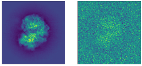
Given a 3D molecule with an electrostatic potential function (henceforth “particle”), the images captured by the electron microscope are modeled as noisy tomographic projections along different orientations. A tomographic projection of the particle onto the x-y plane is defined as . More general tomographic projections are given by a rotation of the potential function followed by projection onto the x-y plane,
| (1) |
where , and we define . Particle images in cryo-EM are typically modeled as follows,
| (2) |
where is a point spread function that is convolved with the projection and is Gaussian noise. See Figure 1 for an example of a tomographic projection. We define the viewing angle of our particle as a unit vector that represents orientation of our particle modulo in-plane rotations (which can be represented as members of ).
1.2 Clustering tomographic projections
The imaging process in cryo-EM involves high-levels of noise. To improve the signal-to-noise ratio (SNR), it is common to cluster the noisy projection images with ones that are similar up to an in-plane rotations. This clustering task is called “2D classification and averaging” in the cryo-EM literature and the clusters are called classes. The results of this stage have multiple uses, including:
- •
-
•
Particle sorting (Zhou et al., 2020), discarding images that belong to bad clusters.
-
•
Visual assessment and symmetry detection.
- •
Existing methods for 2D clustering include the reference-free alignment algorithm that tries to find a global alignment of all images (Penczek et al., 1992), clustering based on invariant functions and multivariate statistical analysis (Schatz and Van Heel, 1990), rotationally invariant k-means (Penczek et al., 1996) and the Expectation-Maximization (EM) based approach of Scheres et al. (2005). All of these methods use the distance metric on rotated images.
Let us consider a simple centroid+noise model, where each image in a cluster is generated by adding Gaussian noise to a particular clean view that is the (oracle) centroid,
| (3) |
In that case the metric is (up to constants) nothing but the log-likelihood of the image patch, conditioned on ,
| (4) |
Under the centroid+noise model, the commonly-used distance metric seems perfectly suitable. However, real particle images have many other sources of variability, including angular differences, in-plane shifts and various forms of molecular heterogeneity. For these sources of variability, the distance metric is ill-suited. See Section 4 for more on this.
In this work we propose to use the Wasserstein-1 metric , also known as the Earthmover’s distance, as an alternative to the distance for comparing particle images. In Section 2 we describe a variant of the rotationally invariant k-means that is based on a fast linear-time approximation of and in Section 3.2 we demonstrate superior performance on a synthetic dataset of Ribosome projections. In Section 4 we analyze the behavior of the and metrics theoretically with respect to angular differences of tomographic projections. In particular we show that the rotationally-invariant metric has the nice property that it is bounded from above by the angular difference of the projections. On the other hand, the metric shows no such relation.
2 Methods
In cryo-EM, in-plane rotations of the molecular projections are assumed to be uniformly distributed, hence is is desirable for the distance metric to be invariant to in-plane rotations. A natural candidate is the rotationally-invariant Euclidean distance,
| (5) |
A drawback of this metric is that visually similar projection images that have a small viewing angle difference can have an arbitrarily large distance. See discussion in Section 4.
To address this, we define a metric based on the Wasserstein- Metric between two probability distributions (Villani, 2003). This metric measures the “work” it takes to transport the mass of one probability distribution to the other, where work is defined as the amount of mass times the distance (on the underlying metric space) between the origin and destination of the mass. More formally, the Wasserstein- distance between two normalized greyscale images is defined as
| (6) |
where is the set of joint distributions on with marginals respectively.
In cryo-EM, the Wasserstein-1 metric has been used to understand the conformation space of 3D volumes of molecules (Zelesko et al., 2020). For clustering tomographic projections, we construct a rotationally-invariant distance to be our clustering metric analogously to Eq. (5)
| (7) |
2.1 Clustering with rotationally-invariant metrics
Algorithm 1 describes a generic rotationally-invariant k-means algorithm based on an arbitrary image patch distance metric . The choice gives the rotationally-invariant k-means of Penczek et al. (1996). By supplying we get a new rotationally-invariant k-means algorithm based on the distance. We choose for the distance as it admits a fast linear-time wavelet approximation as we will see in the next section. For both choices of the metric, we initialize the centroids using a rotationally-invariant k-means++ initialization which we describe in Algorithm 2. When we denote we mean that performs an in-plane rotation of an image. We approximate the space of all in-plane rotation angles by a discrete set of angles.
2.2 Computing the Earthmover’s distance
Computing the distance (also known as the Earthmover’s distance) between two pixels can be formulated as a linear program in variables and constraints. Given images, centers, and rotations for each image and iterations of k-means, we have to compute distances. Computing the distance between two size images using a standard LP solver takes on average of 5 seconds to compute using the Python Optimal Transport Library of Flamary and Courty (2017) on a single core of a 7th generation 2.8 GHz Intel Core i7 processor. Computing the exact distance over all the rotations of all the images over all the iterations is prohibitively slow.
Fortunately, the distance admits a wavelet-based approximation with a runtime that is linear in the number of pixels (Shirdhonkar and Jacobs, 2008). Let be the 2D wavelet transform of . We can approximate the distance between two images by a weighted distance between their wavelet coefficients,
| (8) |
where goes over all the wavelet coefficients and is the scale of the coefficient. This metric is strongly equivalent to . i.e. there exist constants such that for all
| (9) |
Different choices of the wavelet basis give different ratios . We chose the symmetric Daubechies wavelets of order 5 due to the quality of their approximation (Shirdhonkar and Jacobs, 2008). The sum in Eq. (8) was computed with scale up to using the PyWavelets package (Lee et al., 2019).
3 Experimental results
3.1 Dataset generation
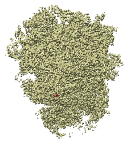
We built a synthetic dataset of 10,000 tomographic projections of the Plasmodium falciparum 80S ribosome bound to the anti-protozoan drug emetine, EMD-2660 (Wong et al., 2014), shown in Figure 1. To generate each image, we randomly rotated the ribosome around its center of mass using a uniform draw of , projected it to 2D by summing over the axis and resized the resulting image to . Finally we added i.i.d. noise to the image at different signal-to-noise (SNR) levels. Given a dataset of images , the SNR is defined as
| (10) |
We produce three datasets to run experiments on by adding noise at SNR values .
3.2 Simulation results
We performed rotationally-invariant 2D clustering on our three datasets using rotationally-invariant k-means++ (Algorithms 1, 2) with the and distance using clusters.
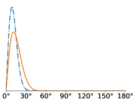
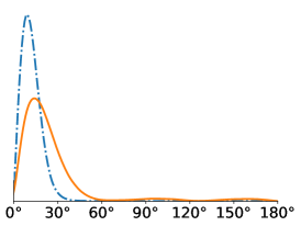
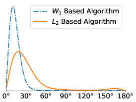
All in-plane rotations at increments of radians were tested in the Algorithm 1. To quantify the difference in performance, we computed the distribution of within-cluster viewing angle differences for all pairs of images assigned to the same cluster. For a molecule like the Ribosome that has no symmetries, we expect these angular differences to be concentrated around zero, since large angular differences typically give large differences in the projection images. For all SNR levels, we see that gives better angular coherence than . Note that some of these distributions have a small peak towards 180 degrees which physically represents our algorithms confusing antipodal viewing angles.
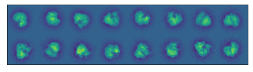
In Figure 3 we show the cluster means of the 8 largest clusters at SNR . Visually, we can see that the algorithm based on produces sharper mean images.
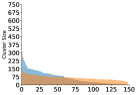
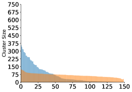
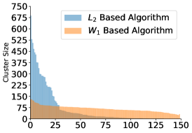
Finally, we examine the occupancy of the clusters. The algorithm provides more evenly sized clusters, whereas for the algorithm we see a few very populated centers and a large dropoff in occupancy in the other clusters.
When clustering images with Gaussian noise, the averages of larger clusters will tend to be less noisy, since the noise variance is inversely proportional to the cluster size. Due to the lower noise levels, more of the images will be assigned to the larger clusters, making them even larger. This “rich get richer” phenomenon has been observed in cryo-EM (Sorzano et al., 2010). It can explain the large differences in occupancy visible in the top panels of Figure 4, despite the fact that the angles were drawn uniformly. The Wasserstein distance is more resilient to i.i.d. noise and this may explain the uniformity in the resulting cluster sizes seen in the bottom panels of Figure 4.
Finally, clustering with the distance does not increase the runtime of the clustering algorithm by much. We include timing results per iteration of k-means with each metric, along with the number of iterations it took for the algorithm to converge in Table 1.
| Metric | k-means (sec/iteration) | (SNR ) | (SNR ) | (SNR ) |
|---|---|---|---|---|
| 1204 s | 13 | 31 | 22 | |
| 1676 s | 23 | 27 | 26 |
3.3 Sensitivity to noise
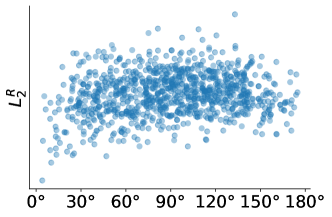
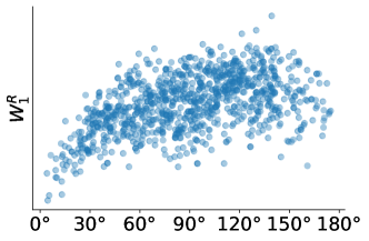
To examine the effect of noise on the and distances, we plot the and distances against the viewing angle difference between projections of the ribosome. In Figure 5 we can see that continues to give meaningful distances under noise compared to the distance.
4 Theory
For a given particle, two tomographic projections from similar viewing angles typically produce images that are similar. Hence, it is desirable that a metric for comparing tomographic projections will a assign small distance to projections that have a small difference in viewing angle. We show that the rotationally-invariant Wasserstein metric satisfies this property.
Proposition 1.
Let be a probability distribution supported on the 3D unit ball and let and be its tomographic projections along the vectors and respectively. Denote by the angle between the vectors, then
| (11) |
where is the rotationally-invariant Wasserstein metric defined in Eq. (7).
See Appendix A for the proof. A similar upper-bound for the rotationally-invariant distance cannot hold for all densities . To see why, consider an off-center point mass. Any two projections at slightly different viewing angles will have a large distance no matter how small their angular difference is. However, for densities with bounded gradients it is possible to produce upper bounds.
Proposition 2.
Let be an upper bound on the absolute gradient of the density. Under the same conditions of Proposition 1 we have
| (12) |
The proof is in Appendix A.
This bound suggests that is a reasonable metric to use for very smooth signals. For non-smooth signals, or signals with very large , this means that there is no guarantee that the distance will assign a small distance between projections with a small viewing angle.
5 Discussion
From our numerical experiments, we see that the rotationally-invariant Wasserstein-1 k-means clustering algorithm produces clusters that have more angular coherence and sharper cluster means than the rotationally-invariant clustering algorithm. Thus, we believe it is a promising alternative to commonly used rotationally-invariant clustering algorithms based on the distance.
Recently, there has been an explosion of interest in the analysis of molecular samples with continuous variability (Nakane et al., 2018; Sorzano et al., 2019; Moscovich et al., 2020; Lederman et al., 2020; Zhong et al., 2020; Dashti et al., 2020). In the presence of continuous variability, it is much more challenging to employ 2D class averaging and related techniques. This is due to the fact that the clusters need to account not only for the entire range of viewing directions but also for all the possible 3D conformations of the molecule of interest. In future work we would like to test the performance of Wasserstein-based k-means clustering for datasets with continuous variability. Wasserstein metrics seem like a natural fit since, by definition, motion of a part of the molecule incurs a distance no greater than the mass of the moving part multiplied by its displacement.
There are many other directions for future work, including incorporating Wasserstein metrics into EM-ML style algorithms (Scheres, 2015), Wasserstein barycenters for estimating the cluster centers (Cuturi and Doucet, 2014), rotationally-invariant denoising procedures (Zhao and Singer, 2014), incorporating translations, experiments on more realistic datasets with a contrast transfer function and analysis of real datasets.
6 Broader impact
Our work demonstrates that the use of Wasserstein metrics can improve the quality of clustering tomographic projections in the context of cryo-electron microscopy. This can reduce the number of images required to produce high quality cluster averages. Improved data efficiency in the cryo-EM pipeline will accelerate discovery in structural biology (with broad implications to medicine) and lower the barriers of entry to cryo-EM for resource-constrained labs around the world.
Appendix A Appendix: proofs
A.1 Proof of Proposition 1
Consider a probability measure on some space and let be a measurable mapping. it naturally induces a measure on its image known as the push-forward measure or image measure , defined by
| (13) |
Lemma 1.
Given two probability distributions on the unit ball ,
| (14) |
where is the tomographic projection in terms of a pushforward measure of defined on onto , and the Earthmover’s distance for each is defined for the underlying probability space.
Proof.
Let be any transportation measure on such that . Let map Lesbegue measurable subsets of to measurable subsets of such that each element in a measurable set of is mapped to . Let where denotes the push-forward operator. . By the change of variables formula for push-forward measures:
| (15) | |||
| (16) | |||
| (17) |
We conclude that
| (18) |
where the last inequality is because any is a valid transportation measure for . ∎
Lemma 2.
Let be tomographic projections of at viewing angles respectively.
| (19) |
Proof.
The second inequality is immediate, since for all we have . We denote the tomographic projection of at orientation as . Without loss of generality, where is the identity matrix and so and . decompose to an in-plane rotation and an out-of-plane rotation (has axis in ).
We observe the chain of inequalities:
| (20) | ||||
| (21) | ||||
| (22) | ||||
| (23) | ||||
| (24) | ||||
| (25) |
The first equality comes from the decomposition of , the second comes from the invariance of to in-plane rotations, the third inequality comes from the definition of , and the fourth equality rewrites . The fifth inequality comes from Lemma 14. The final step of this chain comes from the Monge formulation of the Wasserstein metric (Peyré and Cuturi, 2019), from which it follows that for any two probability distributions on , we have
| (26) |
For , . It is immediate from this statement that using the map we obtain that
| (27) |
Furthermore, for any vector with , we have
| (28) |
where is the angle of rotation of in its axis-angle representation. This gives,
| (29) |
which completes our proof. ∎
Corollary 1.
Let be tomographic projections of at viewing angles respectively.
| (30) |
Which comes from the fact that (Peyré and Cuturi, 2019) from which we obtain and the subsequent chain of inequalities.
A.2 Proof of Proposition 2
Let be differentiable, and . Then for two tomographic projections of , at angles we have
| (31) |
Proof.
This is a consequence of the mean value theorem. Without loss of generality, let us assume that where is the identity matrix and so .
Let . We can decompose into an in-plane component
and an out-of-plane component such that and has its axis of rotation in . Because
is invariant to rotations of , which means that since
| (32) | ||||
| (33) | ||||
| (34) | ||||
| (35) | ||||
| (36) |
The second to last line holds because by the mean value theorem
| (37) |
We observe that the distance the point travels when acted on by is equal to the out-of-plane angle that rotates by multiplied by the distance from to the axis of which is . Thus we can upper bound . Since we achieve the desired upper bound. ∎
References
- Berman (2000) Helen M. Berman. The Protein Data Bank. Nucleic Acids Research, 28(1):235–242, 2000. doi:10.1093/nar/28.1.235.
- Chen and Grigorieff (2007) James Z. Chen and Nikolaus Grigorieff. SIGNATURE: A single-particle selection system for molecular electron microscopy. Journal of Structural Biology, 157(1):168–173, 2007. doi:10.1016/j.jsb.2006.06.001.
- Cheng (2018) Yifan Cheng. Single-particle cryo-EM—How did it get here and where will it go. Science, 361(6405):876–880, 2018. doi:10.1126/science.aat4346.
- Cressey and Callaway (2017) Daniel Cressey and Ewen Callaway. Cryo-electron microscopy wins chemistry Nobel. Nature, 550(7675):167–167, 2017. doi:10.1038/nature.2017.22738.
- Cuturi and Doucet (2014) Marco Cuturi and Arnaud Doucet. Fast computation of Wasserstein barycenters. International Conference on Machine Learning (ICML), 32(2):685–693, 2014.
- Dashti et al. (2020) Ali Dashti et al. Retrieving functional pathways of biomolecules from single-particle snapshots. Nature Communications, 11(1):4734, 2020. doi:10.1038/s41467-020-18403-x.
- de la Rosa-Trevín et al. (2013) J.M. de la Rosa-Trevín et al. Xmipp 3.0: An improved software suite for image processing in electron microscopy. Journal of Structural Biology, 184(2):321–328, 2013. doi:10.1016/j.jsb.2013.09.015.
- Flamary and Courty (2017) Rémi Flamary and Nicolas Courty. POT Python Optimal Transport library, 2017. http://pythonot.github.io.
- Frank (2006) Joachim Frank. Three-Dimensional Electron Microscopy of Macromolecular Assemblies. Oxford University Press, 2006. ISBN 9780195182187. doi:10.1093/acprof:oso/9780195182187.001.0001.
- Frank and Wagenknecht (1983) Joachim Frank and Terence Wagenknecht. Automatic selection of molecular images from electron micrographs. Ultramicroscopy, 12(3):169–175, 1983. doi:10.1016/0304-3991(83)90256-5.
- Grant et al. (2018) Timothy Grant, Alexis Rohou and Nikolaus Grigorieff. cisTEM, user-friendly software for single-particle image processing. eLife, 7(3):377–388, 2018. doi:10.7554/eLife.35383.
- Greenberg and Shkolnisky (2017) Ido Greenberg and Yoel Shkolnisky. Common lines modeling for reference free Ab-initio reconstruction in cryo-EM. Journal of Structural Biology, 200(2):106–117, 2017. doi:10.1016/j.jsb.2017.09.007.
- Heimowitz et al. (2018) Ayelet Heimowitz, Joakim Andén and Amit Singer. APPLE picker: Automatic particle picking, a low-effort cryo-EM framework. Journal of Structural Biology, 204(2):215–227, 2018. doi:10.1016/j.jsb.2018.08.012.
- Lederman et al. (2020) Roy R. Lederman, Joakim Andén and Amit Singer. Hyper-molecules: on the representation and recovery of dynamical structures for applications in flexible macro-molecules in cryo-EM. Inverse Problems, 36(4):044005, 2020. doi:10.1088/1361-6420/ab5ede.
- Lee et al. (2019) G. Lee, R. Gommers, F. Waselewski, K. Wohlfahrt and A. O’Leary. PyWavelets: a Python package for wavelet analysis. Journal of Open Source Software, 4(36):1237, 2019. doi:10.21105/joss.01237.
- Lyumkis (2019) Dmitry Lyumkis. Challenges and opportunities in cryo-EM single-particle analysis. Journal of Biological Chemistry, 294(13):5181–5197, 2019. doi:10.1074/jbc.REV118.005602.
- Lyumkis et al. (2013) Dmitry Lyumkis, Axel F. Brilot, Douglas L. Theobald and Nikolaus Grigorieff. Likelihood-based classification of cryo-EM images using FREALIGN. Journal of Structural Biology, 183(3):377–388, 2013. doi:10.1016/j.jsb.2013.07.005.
- Moscovich et al. (2020) Amit Moscovich, Amit Halevi, Joakim Andén and Amit Singer. Cryo-EM reconstruction of continuous heterogeneity by Laplacian spectral volumes. Inverse Problems, 36(2):024003, 2020. doi:10.1088/1361-6420/ab4f55.
- Nakane et al. (2018) Takanori Nakane, Dari Kimanius, Erik Lindahl and Sjors HW Scheres. Characterisation of molecular motions in cryo-EM single-particle data by multi-body refinement in RELION. eLife, 7:1–18, 2018. doi:10.7554/eLife.36861.
- Penczek et al. (1992) Pawel Penczek, Michael Radermacher and Joachim Frank. Three-dimensional reconstruction of single particles embedded in ice. Ultramicroscopy, 40(1):33–53, 1992. doi:10.1016/0304-3991(92)90233-A.
- Penczek et al. (1996) Pawel A. Penczek, Jun Zhu and Joachim Frank. A common-lines based method for determining orientations for N>3 particle projections simultaneously. Ultramicroscopy, 63(3-4):205–218, 1996. doi:10.1016/0304-3991(96)00037-X.
- Peyré and Cuturi (2019) Gabriel Peyré and Marco Cuturi. Computational Optimal Transport: With Applications to Data Science. Foundations and Trends® in Machine Learning, 11(5-6):355–607, 2019. doi:10.1561/2200000073.
- Punjani et al. (2017) Ali Punjani, John L. Rubinstein, David J. Fleet and Marcus A. Brubaker. cryoSPARC: algorithms for rapid unsupervised cryo-EM structure determination. Nature Methods, 14(3):290–296, 2017. doi:10.1038/nmeth.4169.
- Rohou and Grigorieff (2015) Alexis Rohou and Nikolaus Grigorieff. CTFFIND4: Fast and accurate defocus estimation from electron micrographs. Journal of Structural Biology, 192(2):216–221, 2015. doi:10.1016/j.jsb.2015.08.008.
- Schatz and Van Heel (1990) Michael Schatz and Marin Van Heel. Invariant classification of molecular views in electron micrographs. Ultramicroscopy, 32(3):255–264, 1990. doi:10.1016/0304-3991(90)90003-5.
- Scheres (2012) Sjors H.W. Scheres. RELION: Implementation of a Bayesian approach to cryo-EM structure determination. Journal of Structural Biology, 180(3):519–530, 2012. doi:10.1016/j.jsb.2012.09.006.
- Scheres (2015) Sjors H.W. Scheres. Semi-automated selection of cryo-EM particles in RELION-1.3. Journal of Structural Biology, 189(2):114–122, 2015. doi:10.1016/j.jsb.2014.11.010.
- Scheres et al. (2005) Sjors H.W. Scheres, Mikel Valle and J.-M. Carazo. Fast maximum-likelihood refinement of electron microscopy images. Bioinformatics, 21(Suppl 2):ii243–ii244, 2005. doi:10.1093/bioinformatics/bti1140.
- Shirdhonkar and Jacobs (2008) Sameer Shirdhonkar and David W. Jacobs. Approximate earth mover’s distance in linear time. In Conference on Computer Vision and Pattern Recognition (CVPR), pages 1–8. IEEE, 2008. doi:10.1109/CVPR.2008.4587662.
- Singer and Sigworth (2020) Amit Singer and Fred J. Sigworth. Computational Methods for Single-Particle Electron Cryomicroscopy. Annual Review of Biomedical Data Science, 3(1):163–190, 2020. doi:10.1146/annurev-biodatasci-021020-093826.
- Sorzano et al. (2019) C. O. S. Sorzano et al. Survey of the analysis of continuous conformational variability of biological macromolecules by electron microscopy. Acta Crystallographica Section F Structural Biology Communications, 75(1):19–32, 2019. doi:10.1107/S2053230X18015108.
- Sorzano et al. (2010) C.O.S. Sorzano et al. A clustering approach to multireference alignment of single-particle projections in electron microscopy. Journal of Structural Biology, 171(2):197–206, 2010. doi:10.1016/j.jsb.2010.03.011.
- Tang et al. (2007) Guang Tang et al. EMAN2: An extensible image processing suite for electron microscopy. Journal of Structural Biology, 157(1):38–46, 2007. doi:10.1016/j.jsb.2006.05.009.
- Villani (2003) Cédric Villani. Topics in Optimal Transportation, volume 58 of Graduate Studies in Mathematics. American Mathematical Society, Providence, Rhode Island, 2003. ISBN 9780821833124. doi:10.1090/gsm/058.
- Vinothkumar and Henderson (2016) Kutti R. Vinothkumar and Richard Henderson. Single particle electron cryomicroscopy: trends, issues and future perspective. Quarterly Reviews of Biophysics, 49:1–25, 2016. doi:10.1017/S0033583516000068.
- Wong et al. (2014) Wilson Wong et al. Cryo-EM structure of the Plasmodium falciparum 80S ribosome bound to the anti-protozoan drug emetine. eLife, 3(3):1–20, 2014. doi:10.7554/eLife.03080.
- Zelesko et al. (2020) Nathan Zelesko, Amit Moscovich, Joe Kileel and Amit Singer. Earthmover-Based Manifold Learning for Analyzing Molecular Conformation Spaces. In International Symposium on Biomedical Imaging (ISBI), pages 1715–1719. IEEE, 2020. doi:10.1109/ISBI45749.2020.9098723.
- Zhao and Singer (2014) Zhizhen Zhao and Amit Singer. Rotationally invariant image representation for viewing direction classification in cryo-EM. Journal of Structural Biology, 186(1):153–166, 2014. doi:10.1016/j.jsb.2014.03.003.
- Zhong et al. (2020) Ellen D Zhong, Tristan Bepler, Joseph H Davis and Bonnie Berger. Reconstructing continuous distributions of 3D protein structure from cryo-EM images. In International Conference on Learning Representations (ICLR), pages 1–20, 2020.
- Zhou et al. (2020) Ye Zhou, Amit Moscovich, Tamir Bendory and Alberto Bartesaghi. Unsupervised particle sorting for high-resolution single-particle cryo-EM. Inverse Problems, 36(4), 2020. doi:10.1088/1361-6420/ab5ec8.