Wave-Packet Effects: A Solution for Isospin Anomalies
in Vector-Meson Decay
Abstract
There is a long-standing anomaly in the ratio of the decay width for to that for at the level of . A similar anomaly exists for the ratio of to at . In this study, we reassess the anomaly through the lens of Gaussian wave-packet formalism. Our comprehensive calculations include the localization of the overlap of the wave packets near the mass thresholds as well as the composite nature of the initial-state vector mesons. The results align within confidence level with the Particle Data Group’s central values for a physically reasonable value of the form-factor parameter, indicating a resolution to these anomalies. We also check the deviation of a wave-packet resonance from the Briet-Wigner shape and find that wide ranges of the wave-packet size are consistent with the experimental data.
1 Introduction
There is a long-standing anomaly (discrepancy between experimental and theoretical results) in the ratio of the decay width for to that for . A similar but weaker anomaly exists for the ratio of to . On the other hand, the ratio of to is consistent with the standard theoretical predictions.
At the quark level, these processes are111 Here and hereafter, we omit , , and . is sometimes written as . We do not distinguish the weak-interaction eigenstates and the mass eigenstates , neglecting the small violating effects. Other processes have even smaller violating effects and we neglect them too.
which can be summarized as , where and are vector and pseudo-scalar mesons, respectively, and and are heavy (, , ) and light (, ) quarks, respectively. This ratio of decay widths is theoretically clean because most of the quantum-chromodynamics (QCD) corrections cancel out between the numerator and the denominator. These decay processes are via strong interaction, and hence in the limit of exact isospin symmetry , the ratio becomes unity. The isospin violation makes a deviation from unity.
We name the ratio of the widths as222 In the original Ref. [1], the first two of Eq. (2) are given in its inverse and we have inverted them in Eq. (2). In the theoretical literature, the ratio (1) of charged to neutral modes is mainly used, and we follow it for ease of comparison.
| (1) |
The experimental results are combined by the Particle Data Group (PDG) [1]:333 In the evaluation of [1], the following isospin symmetry among, e.g., and is assumed. The extent to which the isospin symmetry is valid in hadronic decays is debatable [Private communication with Dr. Akimasa Ishikawa].
| (2) |
The theoretical prediction of the decay rates for and is based on the plane-wave formalism so far. The tree-level result of the chiral perturbation theory reads
| (3) |
where () is the coupling between and () and , , and are the masses of , , and , respectively. Even if we assume an isospin-symmetric coupling , the difference in the pseudo-scalar-meson masses results in a deviation in from unity: Putting the mass values in Ref. [1],444 Concretely, assuming the standard error propagation for the twice pseudo-scalar mass. The total decay widths are we obtain
| (4) |
Comparing Eqs. (2) and (4), we see that the isospin-symmetric limit for the coupling results in the anomaly at the level of , , and for , , and , respectively.
We briefly review the theoretical accounts for the anomaly within plane-wave formalism. For , it turned out that radiative corrections make the anomaly more significant [2]: The standard quantum-electrodynamics (QED) corrections make the theoretical prediction of the ratio 4 % larger, and isospin-breaking corrections to the ratio further make it “some 2 %” [2] larger, leading to a larger anomaly of roughly assuming that the error is dominated by that in Eq. (2). In Ref. [3] the authors introduce a smeared decay rate that is a function of the energy difference between the initial and final plane-wave states; this smearing is by the Lorentzian distribution due to the inclusion of the width as well as by a phenomenological form factor put by hand to regularize an ultraviolet (UV) divergence; the anomaly for can be explained with a mass parameter in the phenomenological form factor. In Ref. [4], the authors have estimated the effects of the electromagnetic structure of kaons and other model-dependent contributions to the radiative corrections, and the resultant corrections have turned out to be tiny. In Ref. [5], two (a Breit-Wigner and a non-relativistic Lorentzian) types of averaged decay widths over the initial-state energy are introduced with two phenomenologically chosen energy intervals 1.010–1.060 GeV and 1.000–1.100 GeV, to relax the anomaly.
For , another type of averaged decay width is introduced in Ref. [6], and the resultant anomaly has become even more significant. There is no explanation for this anomaly so far.
The above smearing/averaging over the energy provides significant effects because the decay is near the threshold . In situations near the threshold, it is desirable to treat the decay more rigorously by using wave packets for the initial and final states. Recall that the -matrix in the plane-wave formalism contains the energy-momentum-conserving delta function and is theoretically ill-defined when computing the probability rather than the rate. A well-defined decay probability can be calculated only as a transition from a wave packet to a pair of wave packets. This is theoretically more reliable.
In the previous analyses [3, 4, 5], it has been assumed that the transition processes are described by the (plane-wave) rates alone.555 See also Refs. [7, 8] for non-standard approaches within the plane-wave formalisms. In this paper, we present an analysis based on the transition probability of the normalized states, wave packets, without the divergence of the delta-function squared. Concretely, we compute the decay in the Gaussian wave-packet formalism [9, 10, 11, 12, 13]; see also Refs. [14, 15, 16].666 There is an ongoing experimental project directly to confirm this wave-packet effect [17, 18]; see also Ref. [19]. In particular, we include a wave packet effect, called the in-time-boundary effect for the decay, by simply limiting the time-integral of the decay-interaction point to [10]. Here, is the time from which the interaction is switched on. This procedure is proven to provide approximate modeling of the full production process of in the corresponding two-to-two wave-packet scattering, say, [13]; see also Refs. [20, 21, 11, 12, 22, 23, 24] for related discussions.
The organization of this paper is as follows: In Section 2, we will introduce the minimum basics of calculating the (generalized) -matrix that describes wave-packet-to-wave-packet transitions considering the initial state’s decaying nature when wave packets take the Gaussian form. In Section 3, we will review significant properties of the Gaussian wave-packet -matrix. In Section 4, we will compare the theoretical predictions for the ratios of , , and in the wave-packet and the plane-wave formalisms taking into account the form factor of the vector mesons. In Section 5, we will discuss the constraint from the resonant shape in the electron-positron-collider experiments for and . In Section 6, we will provide a summary and further discussions. In Appendix A, we will review the form-factor details for vector mesons used for our analysis. In Appendix B, we will provide the details on how to derive the total probability of under non-relativistic approximations. In Appendix C, a brief review on how to derive the plane-wave decay rate for will be provided. In Appendix D, we will comment on a specific formal limit where the wave-packet decay rate coincides with the plane-wave decay rate. In Appendix E, we will briefly consider the isospin violation on the system.
2 Basics of Gaussian wave-packet formalism
For the near-threshold decay, the velocities in the final state are small, and the overlap of the wave packets becomes more significant in general. Therefore, it is important to take them into account.
Here, we spell out how to compute the probability for the decay in the Gaussian wave-packet formalism. Throughout this paper, we work in the natural units . Readers who are more interested in analyses of experimental results rather than detailed theoretical formulation may skim through this section.
2.1 Wave-packet -matrix
In the Gaussian wave-packet formalism, a transition from an initial wave-packet state to a two-body final wave-packet state is characterized by the following generalized -matrix [9]:
| (5) |
where describes the unitary time evolution from the initial time to the final time
| (6) |
in which T denotes the time-ordering and is the interaction Hamiltonian density in the interaction picture. The local interaction point is integrated in the four-dimensional spacetime. It is noteworthy that the wave-packet states and are normalizable and hence the transition amplitude (5) is finite, unlike in the ordinary plane-wave formalism.777 See “Discussion” subsection in Ref. [13] for further discussion. Through the Dyson series expansion of , a perturbative -matrix can be systematically constructed at any order of perturbation using Wick’s theorem, as in the plane wave case [11]. Throughout this paper, the subscripts 0, 1, and 2 denote , , and , respectively.
A free Gaussian wave packet is characterized by a set of parameters , where is the mass; is the width-squared; and is a reference time at which the wave packet takes the Gaussian form with the central values of the peak position and momentum .
Within the chiral perturbation theory, the effective-interaction-Hamiltonian density is
| (7) |
where , , , and are the fields representing the vector meson, the charged pseudo-scalar mesons, the neutral pseudo-scalar meson, and its antiparticle, respectively, and and are the vector-meson effective couplings to the charged pseudo-scalars and to the neutral pseudo-scalars, respectively. In this paper, we take the isospin-symmetric limit,
| (8) |
with which the effective coupling takes the form in the momentum space
| (9) |
where , , and are the four-momenta of the vector meson , the pseudo-scalar meson , and its antiparticle , respectively, and is the polarization vector of the vector meson with being its helicity.888 In Eq. (9), stands for the four-momentum of , with its subscript denoting the initial particle. We use the same letter for the particle label of the neutral pseudo-scalar, with its zero denoting its charge. The distinction should be apparent from the context.
In this paper, we investigate the transition from an off-shell initial state for to an on-shell final state for , having an off-shell energy and on-shell ones , , respectively:999 This procedure of introducing is equivalent to the Weisskopf-Wigner approximation [25, 26]. See Ref. [27] for its inclusion in the Gaussian wave-packet formalism.
| (10) |
where and are the masses of and , respectively; is the on-shell energy of ; and is the “decay width” of , or more precisely, the imaginary part of its plane-wave propagator divided by ; see Ref. [13] for detailed discussion; see also footnote 13. Throughout this paper, we take the narrow-width approximation for as in Eq. (10).101010 Theoretically, is obtained as the imaginary part of the plane-wave propagator at the loop level. See footnote 13. Here, the off-shell should eventually be regarded as an intermediate state for a scattering process that includes the production of , which necessarily introduces the in-time-boundary effect appearing below.
Their wave functions take the form
| (11) |
where is a wave-function (field) renormalization factor for due to its offshellness111111 shows a factor that accounts for the possible extra decrease of the norm of the initial state due to the off-shellness . Anyway, will drop out of the final ratio of the decay probabilities. and
| (12) |
describes the location of the center of the wave packet at a time with the central velocity
| (13) |
Now, it is straightforward to compute the -matrix from Eq. (5) at the leading order in the Dyson series (6) with the effective Hamiltonian (7) from the wave functions (2.1) [11]:
| (14) |
where the notation follows Eq. of Ref. [11] (see also below for a short summary).121212 In Eq. (14), we have dropped the overall phase factor which is irrelevant to the calculation of the probability, while properly taking into account the real damping factor coming from the imaginary part of ; see Eq. (2.1). Differences from the previous calculation [11] are the following four points: First, the coupling is changed to . Second, the “decay width” of is included as the phenomenological factor ,131313 When one includes the production process in the amplitude, e.g., as , the result does not change whether we expand the complete set of intermediate states of by the Gaussian-wave-packet or plane-wave bases; see Sec. 2.3 in Ref. [12]. The imaginary part of the plane-wave propagator of appears through loop corrections, and when translated to the decay process , its effect can be expressed as the phenomenological factor in the plane-wave formalism. Here, we also phenomenologically take into account the exponentially decaying nature of the initial wave packet of through the channel that is common to the plane-wave decay, namely, through the bulk effect that appears below. See also footnote 9. where is the initial time from which starts to exist.141414 is indeed irrelevant in the sense that the time-translational invariance results in the dependence of the final result only on the difference . Furthermore, this dependence on cancels out between the numerator and denominator of the final ratio of the decay probabilities, as we will see. (Physically, we would expect .) Third, in Eq. (2.1) is introduced. Fourth, we have included a phenomenological form factor due to the composite nature of :
| (15) |
where describes a typical length scale of the compositeness of ; see Appendix A. The normalization is such that becomes unity for .
Now we provide a brief introduction to other variables in the first two lines of (14) (see Section 3.1 of [11] for more details):
-
•
is a typical spacial size of the region of interaction:
(16) -
•
is a typical temporal size of the interaction region:151515 We adopt the following notation for arbitrary scalar and vector variables and , respectively:
(17) -
•
is the time of intersection of the three wave packets:
(18) where
(19) is the location of the center of each wave packet at our reference time . As mentioned above, each wave packet takes the Gaussian form centered at at its reference time .
-
•
is called the overlap exponent, which provides the exponential suppression when wave packets are separated from each other:
(20) -
•
We write the deviation of energy-momentum from the conserved values (for their central values of wave packets)
(21) where is the “shifted energy” of each packet.
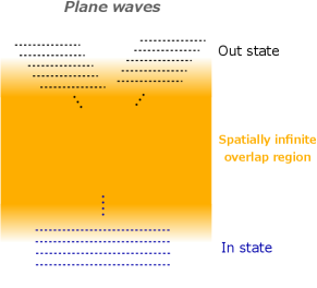
A schematic figure is shown in the left panel of Fig. 1, compared with the plane-wave counterpart in the right.
After the square completion of and the analytic Gaussian integration over in (14), as made in [11], we represent the -matrix as follows:
| (22) |
where the window function is defined as161616 In Eq. (23), on the right-hand side is replaced from the original definition of in [11] as .
| (23) |
with
| (24) |
being the Gauss error function. The window function becomes unity for and zero for and for . For a given configuration of in and out states, which fixes the value of , the time regions ,171717 More precisely, the bulk region is the one satisfying and . , and are called the bulk, in-time-boundary, and out-time-boundary regions, respectively. In the phenomenological analysis below, we will neglect the out-time-boundary contributions as we will discuss.
2.2 Differential decay probability
From the -matrix (22), the differential decay probability can be derived as
| (25) |
where we have taken the average over the helicity , which results in the helicity-averaged effective coupling:
| (26) |
Here, the last equality further assumes the vanishing initial momentum . We will compute the integrated decay probability under this assumption in Sec. 2.3 and in Appendix B.
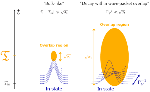
Hereafter, we assume both the following conditions
| (27) |
Physically, each of these conditions is satisfied when at least one of the following three conditions is met:
-
•
(or ) when the interaction time is apart enough from (or ) compared to the temporal width of the overlap , which typically corresponds to the “bulk-like” case (Fig. 2, left);
-
•
when the “mean lifetime through bulk effect” is much shorter than the temporal width of the overlap region , which typically corresponds to the so-to-say “decay within wave-packet overlap” case (Fig. 2, right);
-
•
when the deviation from the conservation of the shifted-energy, , is much larger than the inverse of the temporal width of the overlap , namely the “violation of shifted-energy” case.
This assumption (27) is made for simplicity, and there is no obstacle to using the full form (23) in the numerical computation in principle, but the result would remain the same approximately because this is anyway satisfied in the ordinary bulk-like case as well as when anything interesting happens around the (in-)time-boundary.
Under the assumption (27), the following asymptotic form is obtained [11]:
| (28) |
where we have defined the “bulk window function”
| (29) |
in which the sign function for a complex variable is
| (30) |
Here and hereafter, and denote the real and imaginary parts, respectively. Equation (29) describes the ordinary “bulk contribution” for the quantum transition from the in to out states in the time period . The second and third terms of Eq. (28) show the contributions near the in and out time boundaries and , respectively. More explicitly,181818 Precisely speaking, Eq. (31) is given except right at the boundary or , which is rather a peculiarity of how to define a boundary value and is out of our current interest.
| (31) |
Because the contribution from the out-time-boundary is suppressed by the extra dumping factor in the differential probability (25),191919 Here, we physically assume with ; see also footnote 14. it is safe to neglect the out-time-boundary contribution, and we can take
| (32) |
with which the second line in Eq. (28) goes down to zero. With this limit, reads
| (33) |
where
| (34) | ||||
| (35) | ||||
| (36) |
The three functions , and describe the square of the bulk term, the square of the in-time-boundary term, and the interference between the bulk and in-boundary terms, respectively.
2.3 Integrated decay probability
To compare the theoretical predictions in the Gaussian wave-packet formalism with the experimental results in Eq. (2), we integrate the differential decay probability (37) over the whole position-momentum phase space of the final-state pseudoscalar mesons, namely, over , , , and :
| (39) |
We focus on the situation where these integrals can be performed analytically using the saddle-point approximation; see e.g. Ref. [11]. In the current setup, we can safely take non-relativistic approximations in the kinematics of the system because the mass difference is small.
Here, we only list the final form of the three types of contributions to the integrated decay probability: the bulk, boundary, and interference contributions. These calculations’ details are provided in Appendix B. For later convenience, we define a common dimensionless factor for all of , , and :
| (40) |
2.3.1 Bulk contribution
Integrating the bulk contribution in Eq. (37), we obtain
| (41) |
where
| (42) | ||||
| (43) | ||||
| (44) |
We note that the wave packet size of the decaying particle drops out of this expression at this order of the saddle-point approximation.
2.3.2 Boundary contribution
2.3.3 Interference contribution
Integrating the interference contribution in Eq. (37), we obtain
| (48) |
where the definition of new parameters is as follows:
| (49) | ||||
| (50) | ||||
| (51) | ||||
| (52) | ||||
| (53) |
The tilde denotes that the values are evaluated at the saddle point for the interference contribution.
3 Magnitudes of three kinds of contributions
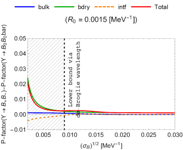
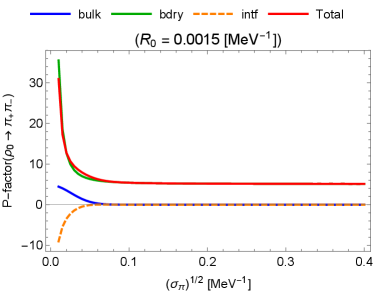
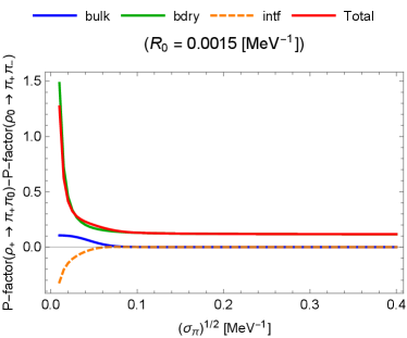
We have seen the magnitudes of the three kinds of contributions to the integrated probability from the bulk part in Eq. (41), from the boundary part in Eq. (45), and from the bulk-boundary interference in Eq. (48). Hereafter, we call the following three ratios the P-factors:
| (54) |
where the common given in Eq. (40) is factored out.
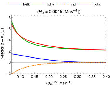
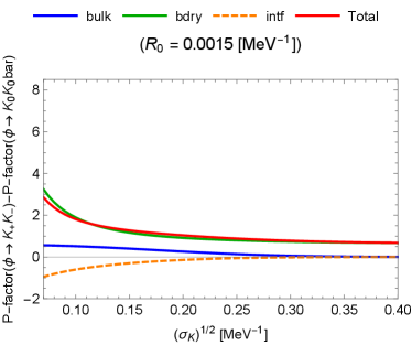
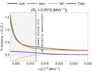
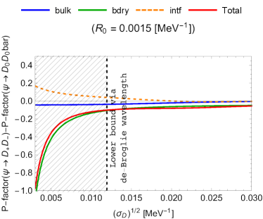
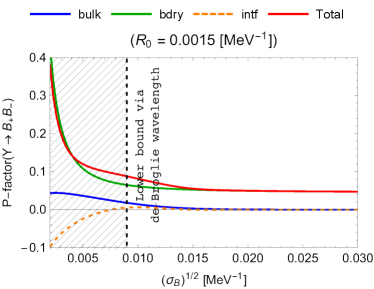
In Fig. 3, the P-factors (54) are shown for the following cases, with a typical value for (see Appendix A):
-
•
and (1st row),
-
•
and (2nd row),
-
•
and (3rd row).
We remind that all of , , and do not depend on within the non-relativistic saddle-point approximation; see Appendix B for details.
From Fig. 3, we can read the following properties:
-
•
If the magnitude of is relatively low, the three kinds of the P-factors are of the same order.
-
•
When is a certain magnitude, the bulk contribution is exponentially suppressed, while the boundary contribution takes almost the same value, where the interference part is negligible. For such a and other higher choices of it, the boundary part dominates.
-
•
Physically, the wave-packet treatment of the decay product breaks down when the wave-packet size is shorter than the de-Broglie wavelength of :
(55) where is the expectation value in the bulk part in Eq. (42). It is straightforward to estimate it for each decay process:
(56) The theoretically excluded region is depicted by the hatched region.
-
•
The differences in the P-factors between the charged-meson and neutral-meson final states are sizable for higher- regions.
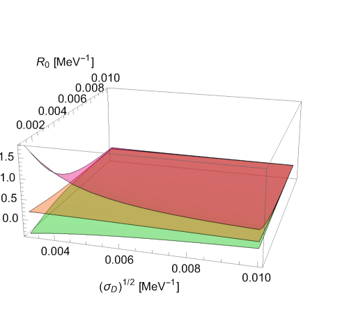
To clarify the dependence on , we prepare the surface plots for the bulk, boundary, and interference parts of the P-factors for as a typical example as Fig. 4. Here, the following properties are observed: (i) The magnitude of each part becomes larger for a smaller and a smaller ; (ii) In the entire domain of and , the boundary part exceeds the bulk part in magnitude.
In Fig. 5, we have also plotted the P-factors for and by adopting the same formulas (41), (45) and (48) for a purpose of qualitative comparison between the decays with narrow phase spaces (, , and ) and that with broad phase spaces (), knowing that it is speculative whether we can still use the non-relativistic approximation.202020 We set and remind , and . We also remind the property that the decay channel is prohibited by the conservation of the isospin. As expected, the difference between and is small since the magnitude of the isospin breaking is much smaller even for a smaller .
4 Analysis of ratio of decay probabilities
In this section, we discuss the ratio of decay probabilities for three vector mesons , , and in the wave-packet formalism. We compare each with the PDG result and find an agreement around a reasonable value of of the form factor (for the compositeness of ). In particular, the 9.5 discrepancy for is dramatically ameliorated. We find that the effect of the form factor is significant in both the wave-packet and plane-wave formalisms.
4.1 Wavepacket analysis
We estimate the wave-packet counterparts of the ratio of the decay rates defined in Eq. (1) for the three vector mesons:
| (57) |
where we ignored the tiny CP-violation effect in . We note that the ratio does not depend on the wave-function (field) renormalization factor (accounting for the offshellness of the vector meson ), nor on the decay factor . Also, we take the isospin-symmetric limit in the couplings as introduced in Eq. (8), and the dependence on the coupling is dropped off. For further comparison, we also define a “bulk” ratio:
| (58) |
which contains the wave-packet contribution only from the bulk part. Also, we introduce the ratio without interference:
| (59) |
4.2 Wavepacket results
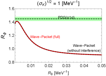
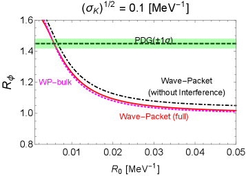
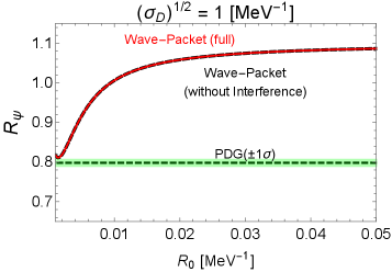
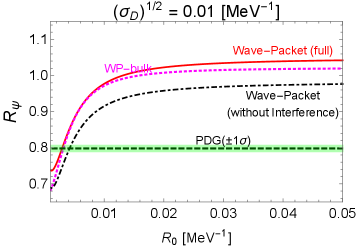
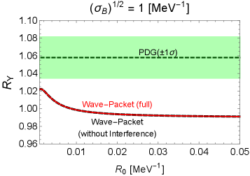
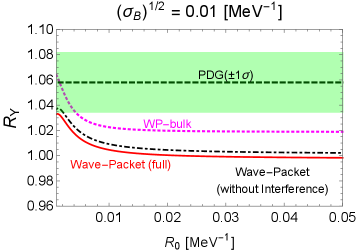
In Figs. 6, 7, and 8, we show the wave-packet results for the decay probability ratios of , , and , respectively. Several comments are in order:
-
•
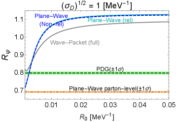
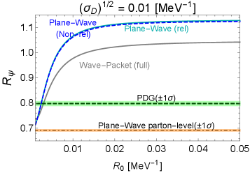
For the decay in Fig. 6, the full wave-packet result in the red solid line can fit the PDG result around the form-factor size and for the wave-packet size of the decay product and , respectively.
-
•
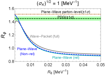
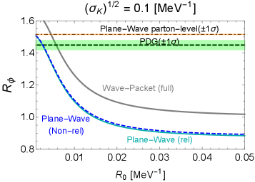
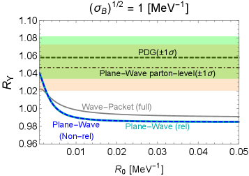
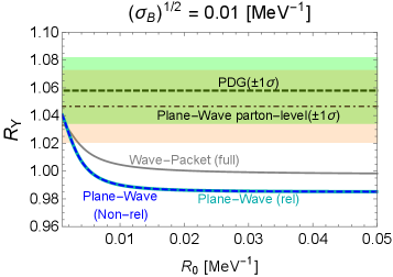
For the decay in Fig. 7, the full wave-packet result in the red solid line can fit the PDG result around the form-factor size and for the wave-packet size of the decay product and , respectively.
-
•
For the decay in Fig. 8, the full wave-packet result in the red solid line can fit the PDG result around the form-factor size and for the wave-packet size of the decay product and , respectively.
-
•
As discussed in Fig. 3, if is sufficiently large, the bulk contribution becomes exponentially suppressed compared to the boundary one. In this regime, we may still formally evaluate the ratio between the (exponentially small) bulk contributions of and :
(60) where the exponent is from Eq. (43). This ratio becomes either exponentially large or small due to the mass difference between and , where the magnitude of the exponents is much greater than . For example, we obtain and if we estimate to be larger than the smallest radius of an electron in atoms that interact with decay products of , namely, the Bohr radius divided by a typical atomic number of the detector atoms, say, and for lead and iron with and 26, respectively. As introduced, the experimental results of , , and are around unity, and they disagree with , both for and . So, the curves are completely out of the depicted ranges of the left panels of Figs. 6, 7, and 8.
4.3 Planewave analysis
For a comparison with the wave-packet results, we also show results with the plane-wave decay rate (see Eq. (168) in Appendix C), taking into account the relativistic form factor (103). The resultant plane-wave ratio becomes
| (61) |
where the parton-level contribution to the ratio is
| (62) |
and the other factor is from the relativistic form factor (103) written in terms of the masses and .
For another comparison, we will also show analyses using its non-relativistic approximated form:
| (63) |
with
| (64) |
where “” represents the operation of taking the non-relativistic approximation and denotes equality under the non-relativistic approximation. The contributions from the form factor are not canceled out in .212121 A similar factor is taken into account in Ref. [3] as a purely phenomenological cutoff factor of a divergent integral within the plane-wave formalism. Note that the ratio (63) can be obtained from the wave-packet counterpart by taking the limits and in ; see Appendix D for details.
4.4 Plane-wave results
We provide comments on the plane-wave results shown in Figs. 9, 10, and 11 below:
-
•
For all of the vector mesons, , , and , the parton-level ratios (4) (under the isospin-symmetric limit for the couplings,222222 Here, we are assuming the isospin-symmetric limit in the sense of Eq. (8) for both the wave-packet and plane-wave calculations. without taking into account the form factor) are disfavored with the PDG’s central values at the level of , , and , respectively.
-
•
On the other hand, when the form-factor effect is included, which is compulsory since the vector mesons are composite particles, we can see agreements with the PDG’s results. It suggests the importance of the form factor in addressing the ratio, where its effect is not fully canceled. Also, we can confirm that the non-relativistic results approximate their relativistic counterparts well for the current system.
-
•
We can find appropriate ranges of the form-factor parameter , where theoretical predictions agree with the PDG’s results for both the full wave-packet and plane-wave curves. For each vector meson, the favored regions of for the wave packet and the plane wave are close to each other but different.
The calculation based on the plane wave works successfully, even though the presumption of free plane waves characterizing initial and final states is, at most, a viable approximation. The wave packet-based calculation provides a comprehensive approach, accounting for all aspects of the quantum nature inherent in the initial and final states, thereby enhancing its reliability. It would be important to precisely discuss the theoretically valid region of , which depends on many details on the strong interaction. We leave this point for future research.
Note that we also briefly consider the isospin violation on the system, where the result is separately available in Appendix E since it might be out of our main interest.
5 Constraint from the shape of vector-meson resonances
In general, it is expected that the resonance shape of is modified by the inclusion of the wave packet effects. That is, vector mesons, produced as resonances in electron-positron colliders, are subjected to a shape-fitting process. This section addresses the constraint on the wave-packet size of pseudoscalar mesons through the resonance shape of the process . Sufficiently precise resonance data from experiments is available for and , facilitating this purpose. However, detailed resonance data for is currently unavailable. Consequently, our focus is maintained on the instances of and . Our analysis in this section is meant to be a brief consistency check, assuming the factorization of the production and decay processes of in both the wave-packet and plane-wave formalisms, and hence is confined to data around the peak.
5.1 Invariant mass distribution of decaying vector-meson wave packet
First, we summarize the invariant mass distribution of the decaying vector-meson when the Gaussian wave packet describes the decaying state.
We define a Lorentz-invariant mass squared for the pair of pseudo-scalars in the final state:
| (65) |
where is the magnitude of with for (see Eq. (108) in Appendix B). We will use
| (66) |
which results in
| (67) |
where we have approximated that decays at rest in the last step.
It is straightforward to derive the following forms after integrating Eq. (38) over the final state phase space, except for , under the current non-relativistic approximation, which is easily rewritten as the invariant mass distribution by use of Eq. (67):
| (68) |
where
| (69) | ||||
| (70) | ||||
| (71) |
Here, we consider the distribution of instead of due to the convenience of comparing the wave-packet shape with the non-relativistic Breit-Wigner (BW) shape, which is the well-known resonant shape for the decaying plane wave with the decay rate ; see the next subsection.232323 Experimentally, one may perform a precision experiment by measuring the ratio per each bin near the resonance, in principle:
5.2 Breit-Wigner shape
For the plane-wave calculation, it is well-known that the non-relativistic Breit-Wigner distribution nicely describes the shape of a narrow resonance,242424 The relativistic Breit-Wigner distribution takes which is not used for the calculation. Mandelstam’s variable is equal to .
| (73) |
where , , and are the resonant mass, the total energy in the center-of-the-mass frame, and the total width of an intermediate resonant particle, respectively. Note that
| (74) |
Since we used the non-relativistic approximation, we are adopting the non-relativistic Breit-Wigner shape (73) for comparison.
5.3 Method of analyzing resonant shape
We assume the following factorization for the resonant production, where the cross-section of the resonant production of and its subsequent decay into and , , can be factorized in the wave-packet (WP) and plane-wave (PW) formalisms, respectively as
| (75) | ||||
| (76) | ||||
| (77) |
where we consider the two cases for PW with and without the form factor (FF); the two cases are discriminated by the short-hand notations “PW-FF” and “PW-Parton”. For the form-factor part of (77), we used the relation in Eq. (66) to convert to .
, , and possess the mass dimension of minus one and describe the factorized production part via the collision at the center-of-the-mass energy . Here, we take these three factors to be independent of since the primal structure of the resonance is in or , and we use only the data points near the peak of a resonance.252525 As is widely known, under the narrow-width approximation in the plane-wave calculation at the resonant peak , we can derive the factorized form explicitly: refer to, e.g., Chapter 16 of [28]. And at this point, is determined as Also, we note that the width-to-mass ratios of the vector mesons take and , where the adaptation of the narrow-width approximation is justified. We will take and for in Eq. (73) as and , respectively; see also Eq. (74). The actual analysis for will be done in the following manner:
- •
-
•
In the analysis, we fix the values of and as confirmed by the PDG group [1], while we treat as an unfixed parameter and will determine it through our statistical fit. The isospin-symmetric coupling and the wave-function renormalization factor for , are taken as unity since it can be absorbed into the factor . Furthermore, for simplicity, we focus on , where the exponential decay factor in in Eq. (40) does not work.
-
•
Under the current scheme, has six parameters , has five parameters , and has three parameters , respectively. We will determine them through statistical analysis. We remind ourselves that the vector-meson wavepacket size does not appear in under the saddle-point approximation.
5.4 Result of
In Ref. [29], the latest result of the resonant shape of through measured with the CMD-3 detector in the center-of-mass energy range – was reported, where the Born cross sections of around the resonance are available in Table I of [29]. According to our guideline, we adopt the seven data points from to and adopt the functions:
| (78) | ||||||
where discriminates the seven points of where experimental data is available; and are the central and error of the experimentally-determined cross section at the point , respectively. , and represent the theoretical values of the corresponding cross sections at the energy point identified by .
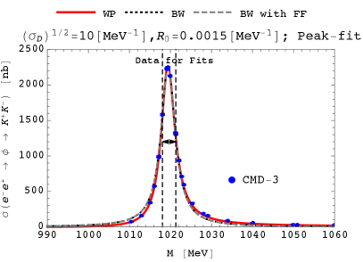
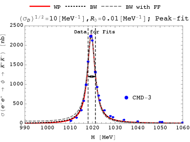
As examples, we show the fitted distributions for the two sets of the fixed parameters and for the left panel of Fig. 12,262626 Note that the value of is a typical value in the current scheme of the form factor (see Appendix A), and its magnitude is favored by the analysis on (see Section 4). and for the right panel of Fig. 12, where the two remaining parameters take the best-fit values, and the values of the over the degrees of freedoms (DOFs), which is currently five, at the best-fit points are calculated as
- •
- •
We comment on the difference between the plane-wave resonant shapes with and without the form factor. Without the factor, the shape obeys the Breit–Wigner distribution (73) and is symmetric under the reflection around the peak (), while taking into account it, the resonant shape becomes asymmetric under the reflection around the peak. The magnitude of the asymmetry is governed by the part of the form factor. So, for a greater , a more significant asymmetry will be realized, as observed in Fig. 12.
Here, we comment on the origin of the “over-” values of : this is because the resolution of the experimental results near the peak is very high, and the current simple scheme for in Eqs. (75), (76) and (77) is not enough for discussing statistical significance precisely. On the other hand, however, we are able to discuss the relative significance between the wave-packet and plane-wave results. According to Eq. (80), the shape of the wave-packet resonant distribution is at least as good as that of the plane-wave resonant distribution at the focused parameter point, where we conclude that the wave-packet result at the first parameter point (for the left panel of Fig. 12) is consistent with the experiment. Note that at the first parameter point, is taken as a typical value in the current scheme of the form factor (see Appendix A), and a wave packet with a greater size looks similar to the plane wave.
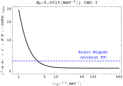
We also see the significance of the wave-packet results over a broad range of under . In Fig. 13, we plot the “minimized” defined by
| (83) |
which measures the statistical significance for . We do not consider the PW-FF case since no sizable difference is generated when , as shown in the left panel of Fig. 12, and the form-factor part does not depend on . Under the simple guideline that a wave-packet result is at least as good as the ordinary plane-wave one, from Fig. 13, we can put the lower bound on as
| (84) |
for .
5.5 Result of
The BaBar, Belle, BES, and CLEO experimental collaborations have provided recent experimental data of the ’s resonance produced by the collision.
-
•
We will adopt the results on [30] of the converting experimental results to the exclusive initial-state-radiation scattering cross-section, , where the following experimental papers are taken into account by BaBar [31], by Belle [32], and by CLEO [33, 34]. “” means the inclusive final states of and .272727 The exclusive initial-state-radiation scattering cross-sections of and are also reported by Babar [35] and by Belle [36]. Since few data points are available inside the focused range , we do not adopt them for our analysis.
-
•
We also take account of the experimental results by BES of the inclusive hadron-production cross-section in [37, 38]. The original data is provided in the form,
(85) where is the lowest-order QED cross section for muon pair production at the total center-of-mass energy . is the QED fine structure constant at the Thomson limit. and are reported in [37] and in [38], respectively. Through the approximation , we can recast the cross section of , as done in [39].
Since the final state is inclusive as , we adopt the following factorized form for the production cross section:
| (86) | ||||
| (87) | ||||
| (88) |
where and are the corresponding branching ratios [1]. The functions are defined as
| (89) |
where and are the central and error of the experimentally-determined cross section at the point of the experiment I, respectively. , and represent the theoretical values of the corresponding cross sections at the energy point identified by .
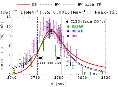
Here, we will see the two examples for the same wave-packet size but two different values for the form-factor parameter . In the left and right panels of Fig. 14, the fitted distributions about the parameters are shown for and , respectively, where the valid ranges of and are fixed as
- •
- •
From Fig. 14, when is large as , the resonant distribution of the wave packet becomes identical with that of the plane-wave without taking into account the form factor. Meanwhile, when , where this size is favored with the agreement in , we observe the deviation from the BW shape in the wave-packet distribution. Note that all three kinds of distributions agree with the experimental data for the larger and smaller .
We comment on the large asymmetry observed in the right panel of Fig. 14, namely the large deviation of “BW with FF” in the low range. As mentioned in the previous subsection, the asymmetry under the reflection around the peak originates from the parts and of the form factors. The realized asymmetry in becomes extensive when is less than the range used for the statistical fit, so this case is considered to be disfavored even though the limited part near the resonant peak is fitted to the experimental results well.
To clarify the experimentally-valid range for , we see the curve of the “minimized” defined by
| (94) |
for . Due to the same reason with the case of for , we skip to consider the PW-FF case. From Fig. 15, we recognize that the range for is consistent with the constraint,
even though the wave-packet shape does not exceed the BW shape in the goodness of fit. To summarize, within the current scheme for the production cross section, no significant bounds on are imposed. This is because, as recognized from Fig. 14, the experimental results still have sizable errors for the ’s resonant shape.
6 Summary and discussion
In this paper, we have discussed the long-standing anomaly in the ratio of the decay rates of the vector mesons and , namely, and , where the strong interaction causes the decay channels, and they measure isospin breakings. If we estimate their theoretical values in the plane-wave formalism without considering the effects originating from the composite nature of the initial-state vector mesons, they are disfavored with the PDG’s central values at the level of and . In particular, there has been no explanation for the latter 9.5 anomaly so far.
The decay channels that we focus on are near the mass thresholds, where the velocities in the final state are small, and hence the localization of the overlap of the wave packets is more significant. Here, we fully take into account such effects in the Gaussian-wave-packet formalism. We carefully clarified the properties of one-to-two-body non-relativistic quantum transitions between normalizable physical states described by Gaussian wave packets under the presence of the decaying nature of the initial state, which is a full-fledged calculation taking into account the essences that are missing in the plane-wave calculations.
The result shows agreement with the PDG’s combined results within confidence level. We conclude that the long-standing anomalies in and are resolved.
In the calculation, the above-mentioned compositeness has been described by the form factor. The agreement is achieved when we appropriately take the form-factor parameter at around the physically reasonable value .
We also analyzed and made a comment on the -vector-meson counterpart , namely , where the plane-wave calculation without considering the above-mentioned composite nature already agrees at the level with the corresponding PDG result due to the smallness of the mass difference between and . The wave-packet result agrees well with the PDG result around the same value of .
We mention that the same form factors can be formally multiplied on the ratio of the plane-wave decay rates in order to partially take into account the wave-packet effects, though the wave-packet approach is more comprehensive in describing quantum transitions. By doing so, around the same value of , the plane-wave results can also be made to agree with the PDG ones.
In general, the shape of a wave-packet resonance deviates from the Briet-Wigner shape, where the magnitude of the deviation depends on the size of wave packets. For and , experimental data is available, and we put constraints on the size. We found that when the size of the wave packets is small, the derivation from the Briet-Wigner shape tends to be sizable. Both for and , wide ranges of the wave-packet size are consistent with the experimental data.
In the decay channels of the vector mesons, the non-relativistic approximation works fine, which simplifies the integrations in the -matrices and the final-state phase spaces in the wave-packet formalism. Many other quantum transitions in high-energy physics are relativistic, and it is worthwhile to establish the general method to perform such integrations without relying on the non-relativistic approximation. Also, analyzing resonant productions precisely requires the full transition probabilities, including production parts. Doing more dedicated analyses on resonant shapes will be another important task.
Acknowledgments
K.I. thanks for useful communications with Dr. Elliott D. Bloom, Dr. Walter Toki, and Dr. Tomasz Skwarnicki on the crystal-ball functions. K.N. thanks Dr. Akimasa Ishikawa for the useful information on experimental details on and Dr. Ryosuke Sato for useful comments on form factors. This work is partially supported by the JSPS KAKENHI Grant Nos. JP21H01107 (K.I., O.J., K.N., K.O.) and JP19H01899 (K.O.).
Appendix
Appendix A Vector-meson form factor
We focus on the following form for a non-relativistic bound state composed of a heavy constituent quark and its anti-particle at a certain time:
| (95) |
where is a wave function for the bound state; and are the Fourier transforms of the momentum-space creation operators of and , respectively, with and being their positions and spins; and is the vacuum; see e.g. Ref. [40].
We consider the following matrix element
| (96) |
where , , and the normalization of the form factor is irrelevant for our purpose.282828 What is relevant is only the product of the normalization of the effective coupling and that of the form factor. Such a normalization factor will be dropped out of the final ratio of the decay probabilities under the isospin-symmetric limit (8).
Hereafter, we assume the separable form
| (97) |
for the heavy and non-relativistic quarks , which have negligible spin-orbital angular momentum interaction. Further, we drop the spin structure , which will be canceled out in the ratio of the neutral to charged rates, and focus on the momentum part.292929 Concretely, the orbital and total angular momenta is (), (), and for , and , respectively; see e.g. “Quark Model” section in Ref. [1].
We adopt an approximate form of the wave function of the (-wave) ground state under a Coulomb potential in the position space:
| (98) |
where , the parameter describes a typical length scale of the bound state discussed below, and is the irrelevant normalization factor mentioned above. Its Fourier-transform is
| (99) |
where we used . In this paper, we choose such that :
| (100) |
This form is also introduced in Ref. [3] to cut off a UV divergence in the plane-wave computation. The treatment in Refs. [4, 5] is equivalent to taking this form factor to be unity.
Here, a vector meson decays into two light pseudo-scalar mesons and . We approximate the mass and momentum for each psuedoscalar () by those of the constituent quark (): and (), respectively. In this paper, we focus on the situation where the masses of the two pseudo-scalar mesons are almost the same (due to the approximated flavor-isospin symmetry), and the mass relation is near the decay threshold,
| (101) |
Therefore, we can treat the process as a non-relativistic one, and thus, we conclude that
| (102) |
thereby,
| (103) | ||||
| (104) |
where and are the (non-relativistic) velocities of and , respectively.
Finally, we reach the spin-independent dimensionless function suitable for our purpose,
| (105) |
This is the form factor shown in Eq. (15) for the matrix elements of the meson decays (with ) in the rest system.
Now we estimate a typical value of the parameter in Eq. (98). The quarkonium potential can be approximated by a sum of the confining linear potential and the QCD Coulomb potential
| (106) |
where is known as [40] and is the QCD fine structure constant. For the domain where ,303030 Here, we have put at the scale GeV [41]. the wave function can be approximated by the Coulomb form (98). One can estimate by equating the potential and kinetic energies, , where . Since is much smaller than the typical energy scale GeV of the potential, the typical distance can be estimated by equating two terms in the right-hand side of Eq. (106): . The use of Coulomb wave function (98) is marginally justified, which suffices for our current consideration. See e.g. Ref. [42] for further refinement.
Finally, a typical value of the parameter in Eq. (98) is
| (107) |
Appendix B Details on calculations of
We present detailed computation to obtain the decay probability integrated over the final-state positions and momenta under the rest-frame assumption .
B.1 Variables under non-relativistic limit
As preparation, we show concrete forms of the kinetic variables and parameters, whose physical meaning is given in Section 2.1, under the non-relativistic limit . At first, we define the ‘light-cone’ variables for later convenience:
| (108) |
The kinetic variables are
| (109) |
where the symbol represents the non-relativistic approximation, which we will take later. We also have
| (110) | ||||
| (111) | ||||
| (112) | ||||
| (113) | ||||
| (114) | ||||
| (115) | ||||
| (116) |
Also, we define the variables and
| (117) |
B.2 Bulk contribution
We compute the bulk contribution in Eq. (37). First, we perform the position integrals . As in Ref. [11], we obtain
| (118) | ||||
| (119) | ||||
| (120) | ||||
| (121) |
where becomes a flat direction under the (unphysical) no-decay limit (as considered in [11]), while the other five directions are not flat directions irrespective of :
| (122) |
where we also used Eq. (31) and took the limit . The range of the integration is given by the bulk window function in Eq. (31). After the position integrations, we obtain
| (123) |
where the damping factors and provide the approximate conservation for the mean energy and momentum, respectively.313131 Of course the energy-momentum conservation is fulfilled in itself as a fundamental physical law of nature, in particular, for each partial plane-wave component in the Fourier transforms. So far the expression (123) does not assume nor the non-relativistic approximation given in Sec. B.1.
Next, we perform the momentum integrals under the saddle-point approximation with in the non-relativistic approximation given in Sec. B.1:
| (124) |
where the factor is from the Jacobian and the exponent is
| (125) |
We see that
| (126) |
which implies
| (127) |
Also, we see that
| (128) |
which leads to
| (129) |
Thereby,
| (130) |
The stationary point that satisfies
| (131) |
is found to be
| (132) |
Now, we focus on the kinetic region ( and ) and thus only the first one is relevant in our calculation,
| (133) |
Note that
| (134) |
which goes to zero in the (unphysical) limit . Also, we can see
| (135) |
where under the (unphysical) limit .
We perform the integrals under the saddle-point approximation (putting in the overall factor) as follows:
| (136) |
where we have used the formulas for ,
| (137) | ||||
| (138) |
and the Taylor expansion around one of the stationary points
| (139) |
B.3 Boundary contribution
We compute the boundary contribution in Eq. (37):
| (140) |
where and the range of the integration is since there exists no window function for this boundary term other than the exponential factor.
Now we perform the Taylor expansion of around the saddle point up to the second order
| (141) |
to obtain
| (142) |
which yields
| (143) |
There is no in the exponent, and we will perform the numerical computation for the integral. On the other hand, the saddle point of is located at . With it in mind, we approximate the polynomial part of the integrand by setting other than :
| (144) |
where we define a dimensionless function
| (145) |
with
| (146) |
Now we execute the integral using the formula (137):
| (147) |
where the integral
| (148) |
is convergent.
B.4 Interference contribution
We compute the interference contribution in Eq. (37). We focus on the part including the factor
since the other part can be obtained by taking complex conjugation. At first, we perform the square completion of the part:
| (149) |
where in the last fine, we changed the variable to and took the limit .
In order to use the analytic formula for and ,323232 One of the necessary conditions for this relation is “”. In our case, the set of these conditions is manifestly fulfilled since corresponds to “”.
| (150) |
where is the exponential integral function defined by the principal value of
| (151) |
we add an extra term in the denominator of the integrand of such that
| (152) |
which would underestimate the integral to some extent. Now, we reach the following analytic form
| (153) |
with
| (154) |
Here, we will take the leading term of the expansion around infinity for ,
| (155) |
which leads to
| (156) |
and
| (157) |
We perform the momentum integrals in the non-relativistic limit:
| (158) |
where
| (159) |
This function is similar to , but a factor of the half comes in front of . As in the case of the bulk part, we can see
| (160) |
Stationary points are defined by
| (161) |
and we find one stationary point in the kinetic region ( and ),
| (162) |
Note that
| (163) |
which takes a positive value when is finite, and goes to zero in the (unphysical) limit . Also, we can see
| (164) |
where under the (unphysical) limit .
Appendix C Plane-wave decay rate
From the effective Hamiltonian (7), under the use of the form factor (105), it is immediate to get the following form in the plane-wave formalism for the resting ,
| (168) |
where represents (for ) or (for ) and the magnitude of the final-state momenta in the center-of-mass frame is given as
| (169) |
The form factor part does not take the non-relativistic limit as in Eq. (105), and currently, and thus
| (170) |
Appendix D Comparison with plane-wave decay rate
As shown in Sec. 3, the boundary contribution dominates over the bulk and interference ones in all regions of the parameter space and . This is because of the fast decay of the vector meson due to strong interactions. The fast decay suppresses the contribution from the bulk so that the contribution from the initial time boundary becomes more significant compared to the bulk one.
As mentioned above, the plane-wave decay width is dependent on other theory parameters such as , , and . Therefore, it is meaningless to take an “on-shell” limit with other parameters being fixed. Nevertheless, one might pretend that one can take this unphysical limit, and then one extracts the plane-wave decay width (171):
| (173) |
where the limit of large wave-packet size is taken after the limit .333333 As said above, anyway drops out of the result at this order of the saddle-point approximation. The second equality in Eq. (173) is derived as follows: Under the limit , the two ratios and approach zero since and are not proportional to as shown in Eqs. (45) and (48). When taking the above limits and , the following is satisfied:
| (174) |
as well as the physical requirement from .
In the actual setup, the (unphysical) limit is not good, and we see that the boundary contribution dominates over the bulk one for the parameters corresponding to the real experiments mainly because of the exponential suppression factor .
Appendix E A brief comment on the isospin breaking of the system
We will make a brief comment on the isospin breaking of the system. Here, we define the following ratio,
| (175) |
where we replace to for the calculations of . In Fig. 16, the in terms of the wave packet and the relativistic plane wave is depicted for (Left panel) and (Right panel); see Sections 2.3 and 4.3 for the details of the wave-packet decay probabilities and the plane-wave decay rates, respectively.
First, we mention the experimental inputs that we adopt. As official results reported by the PDG [1],
-
•
Six digits are reported as typical mass scales of the broad-resonant system, where their central values are located from to .
-
•
Also, six digits are shown as typical width scales of the system, where their central values are located from to .
-
•
The difference between and takes .
-
•
The difference between and takes .
Since measures isospin-violating effects, and thus it is insensitive to what is a typical mass scale of the system. So, we simply take and . Based on the mass scale, is estimated by use of the above data on and as
while the central value of is similarly estimated as . As expected and as shown in Fig. 16, can depend on the mass difference sizably.
Next, we discuss the numerical result shown in Fig. 16. As expected, the experimental result is located very near the unity since the vector mesons do not contain heavy quarks. The plane-wave theoretical predictions with and without the form-factor effect show similar results. The wave-packet predictions deviate from the unity several percent upward, showing fewer agreements. Nevertheless, this does not necessarily mean that wave-packet formalism works less effectively for the system than plane-wave formalism because the current wave-packet result is precise only for non-relativistic systems (due to the usage of non-relativistic approximations). Note that the decays and are fully relativistic due to the large difference between the total masses of the initial state and final state. Several percent of theoretical errors are expected from the fully-relativistic wave-packet prediction, which is beyond the scope of this paper. The typical scale of the form factor under the current scheme works well compared with .
Also, we comment on the dependence on in . As typically observed in the curves of “Plane-Wave (rel)” of Fig. 16, the form-factor part of is not sensitive to since the total mass differences between the initial and the final states take almost the same values in and and their final-state phase spaces are wide.
References
- [1] Particle Data Group collaboration, R. L. Workman et al., Review of Particle Physics, PTEP 2022 (2022) 083C01.
- [2] A. Bramon, R. Escribano, J. L. Lucio M. and G. Pancheri, The Ratio / , Phys. Lett. B 486 (2000) 406 [hep-ph/0003273].
- [3] E. Fischbach, A. W. Overhauser and B. Woodahl, Corrections to Fermi’s golden rule in decays, Phys. Lett. B 526 (2002) 355 [hep-ph/0112170].
- [4] F. Flores-Baez and G. Lopez Castro, Structure-dependent radiative corrections to decays, Phys. Rev. D 78 (2008) 077301 [0810.4349].
- [5] V. I. Kuksa, Finite-width effects in the model of unstable particles with a smeared mass, Int. J. Mod. Phys. A 24 (2009) 1185.
- [6] S. Coito and F. Giacosa, Line-shape and poles of the , Nucl. Phys. A 981 (2019) 38 [1712.00969].
- [7] I. Joichi, S. Matsumoto and M. Yoshimura, Time evolution of unstable particle decay seen with finite resolution, Phys. Rev. D 58 (1998) 045004 [hep-ph/9711235].
- [8] A. Yoshimi, M. Tanaka and M. Yoshimura, Quantum dots as a probe of fundamental physics: deviation from exponential decay law, Eur. Phys. J. D 76 (2022) 113 [2107.04670].
- [9] K. Ishikawa and T. Shimomura, Generalized S-matrix in mixed representations, Prog. Theor. Phys. 114 (2006) 1201 [hep-ph/0508303].
- [10] K. Ishikawa and Y. Tobita, Finite-size corrections to Fermi’s golden rule: I. Decay rates, PTEP 2013 (2013) 073B02 [1303.4568].
- [11] K. Ishikawa and K.-Y. Oda, Particle decay in Gaussian wave-packet formalism revisited, PTEP 2018 (2018) 123B01 [1809.04285].
- [12] K. Ishikawa, K. Nishiwaki and K.-y. Oda, Scalar scattering amplitude in the Gaussian wave-packet formalism, PTEP 2020 (2020) 103B04 [2006.14159].
- [13] K. Ishikawa, K. Nishiwaki and K.-y. Oda, New effect in wave-packet scatterings of quantum fields, 2102.12032.
- [14] K. Ishikawa and Y. Tobita, Matter-enhanced transition probabilities in quantum field theory, Annals Phys. 344 (2014) 118 [1206.2593].
- [15] K. Ishikawa, T. Tajima and Y. Tobita, Anomalous radiative transitions, PTEP 2015 (2015) 013B02 [1409.4339].
- [16] N. Maeda, T. Yabuki, Y. Tobita and K. Ishikawa, Finite-size corrections to the excitation energy transfer in a massless scalar interaction model, PTEP 2017 (2017) 053J01 [1609.00160].
- [17] K. Ishikawa, O. Jinnouchi, A. Kubota, T. Sloan, T. H. Tatsuishi and R. Ushioda, On experimental confirmation of the corrections to Fermi’s golden rule, PTEP 2019 (2019) 033B02 [1901.03019].
- [18] R. Ushioda, O. Jinnouchi, K. Ishikawa and T. Sloan, Search for the correction term to the Fermi’s golden rule in positron annihilation, PTEP 2020 (2020) 043C01 [1907.01264].
- [19] R. G. Breene, Line shape, Rev. Mod. Phys. 29 (1957) 94.
- [20] M. Nauenberg, Correlated wave packet treatment of neutrino and neutral meson oscillations, Phys. Lett. B 447 (1999) 23 [hep-ph/9812441].
- [21] N. N. Achasov, Radiative decays of phi meson about nature of light scalar resonances, Nucl. Phys. A 728 (2003) 425 [hep-ph/0309118].
- [22] K.-y. Oda and J. Wada, A complete set of Lorentz-invariant wave packets and modified uncertainty relation, Eur. Phys. J. C 81 (2021) 751 [2104.01798].
- [23] K.-y. Oda and J. Wada, Lorentz-covariant spinor wave packet, 2307.05932.
- [24] H. Mitani and K.-y. Oda, Decoherence in Neutrino Oscillation between 3D Gaussian Wave Packets, 2307.12230.
- [25] V. Weisskopf and E. P. Wigner, Calculation of the natural brightness of spectral lines on the basis of Dirac’s theory, Z. Phys. 63 (1930) 54.
- [26] V. Weisskopf and E. Wigner, Over the natural line width in the radiation of the harmonius oscillator, Z. Phys. 65 (1930) 18.
- [27] K. Ishikawa, T. Nozaki, M. Sentoku and Y. Tobita, Transition Probability for the Neutrino Wave in Muon Decay and Oscillation Experiments, 1405.0582.
- [28] M. Thomson, Modern particle physics. Cambridge University Press, New York, 2013, 10.1017/CBO9781139525367.
- [29] E. A. Kozyrev et al., Study of the process in the center-of-mass energy range - MeV with the CMD-3 detector, Phys. Lett. B 779 (2018) 64 [1710.02989].
- [30] A. G. Shamov and K. Y. Todyshev, Analysis of BaBar, Belle, BES-II, CLEO and KEDR data on line shape and determination of the resonance parameters, Phys. Lett. B 769 (2017) 187 [1610.02147].
- [31] BaBar collaboration, B. Aubert et al., Study of the Exclusive Initial-State Radiation Production of the System, Phys. Rev. D 76 (2007) 111105 [hep-ex/0607083].
- [32] Belle collaboration, J. Brodzicka et al., Observation of a new meson in decays, Phys. Rev. Lett. 100 (2008) 092001 [0707.3491].
- [33] CLEO collaboration, D. Besson et al., Measurement of at MeV, Phys. Rev. Lett. 96 (2006) 092002 [1004.1358].
- [34] CLEO collaboration, G. Bonvicini et al., Updated measurements of absolute and hadronic branching fractions and at MeV, Phys. Rev. D 89 (2014) 072002 [1312.6775].
- [35] BaBar collaboration, B. Aubert et al., Exclusive Initial-State-Radiation Production of the , , and Systems, Phys. Rev. D 79 (2009) 092001 [0903.1597].
- [36] Belle collaboration, G. Pakhlova et al., Measurement of the near-threshold cross section using initial-state radiation, Phys. Rev. D 77 (2008) 011103 [0708.0082].
- [37] M. Ablikim et al., Measurements of the continuum and values in annihilation in the energy region between and GeV, Phys. Rev. Lett. 97 (2006) 262001 [hep-ex/0612054].
- [38] BES collaboration, M. Ablikim et al., Precison Measurements of the Mass, the Widths of Resonance and the Cross Section at , Phys. Lett. B 652 (2007) 238 [hep-ex/0612056].
- [39] N. N. Achasov and G. N. Shestakov, Electronic width of the resonance interfering with the background, Phys. Rev. D 103 (2021) 076017 [2102.03738].
- [40] E. Eichten, K. Gottfried, T. Kinoshita, K. D. Lane and T.-M. Yan, Charmonium: The Model, Phys. Rev. D 17 (1978) 3090.
- [41] A. Deur, S. J. Brodsky and G. F. de Teramond, The QCD Running Coupling, Nucl. Phys. 90 (2016) 1 [1604.08082].
- [42] N. Brambilla et al., Heavy Quarkonium: Progress, Puzzles, and Opportunities, Eur. Phys. J. C 71 (2011) 1534 [1010.5827].