Wavefunctions from Energies: Applications in simple potentials.
Abstract
A remarkable mathematical property – somehow hidden and recently rediscovered –, allows obtaining the eigenvectors of a Hermitian matrix directly from their eigenvalues. That opens the possibility to get the wavefunctions from the spectrum, an elusive goal of many fields in physics. Here, the formula is assessed for simple potentials, recovering the theoretical wavefunctions within machine accuracy. A striking feature of this eigenvalue–eigenvector relation is that it does not require knowing any of the entries of the working matrix. However, it requires the knowledge of the eigenvalues of the minor matrices (in which a row and a column have been deleted from the original matrix). We found a pattern in these sub–matrices spectra, allowing to get the eigenvectors analytically. The physical information hidden behind this pattern is analyzed.
I Introduction
Recently DentonRosetta:19 , precise perturbative calculations of neutrino oscillation probabilities yield a surprising result: given the eigenvalues of the Hamiltonian and its minor sub–matrices, it is possible to write down all the probabilities by a quite simple expression. In a following two–pages paper the authors Denton:19 described and proved this eigenvector–eigenvalue identity (1), which is the subject of the present work. Despite its simplicity and the possible implications, the identity was not broadly well known. Lately, it achieves a blaze of publicity, after a popular article wolcholver:19 reported the unexpected relationship between the eigenvalues and eigenvectors in the neutrino oscillation calculations. The authors of Denton:19 rewrote the paper, adding thirty pages with several proofs of the identity, together with a discussion about its complicated history in the literature, and the reasons for its unawareness. They also showed that the equation appeared in different references, being independently rediscovered in diverse fields. In most cases, the papers were weakly connected, lacking in significant propagation of citations.
The eigenvector–eigenvalue identity Denton:19 relates the eigenvectors of an Hermitian matrix , with its eigenvalues . In this work, it is slightly modified as follows:
| (1) |
where is the component of the normalized eigenvector associated to the eigenvalue . The eigenvalues correspond to the minor of , formed by removing the row and column.
Identity (1) has many remarkable aspects to discuss. We can mention many positive and very promising issues. First, notice that at no point one ever actually needs to know any of the entries of the matrix to calculate its eigenvectors. From the physical point of view, this can be very useful in systems in which the eigenvalues are got by measurements. The most direct application could be the recovering of the electronic densities from the experimental spectra, which is, perhaps, the holy grail of the physical chemistry. Second, it can lead to the development of new numerical methods to diagonalize large matrices, faster and more efficiently. The standard computer routines use much more memory and resources if the eigenvectors are needed, in place of solely the eigenvalues.
However, these two advantages have some weaknesses. Indeed, the values of the original matrix are not needed, but since the expression (1) involves the minors , this statement is not completely straight. It will be undisputed, only if the minor’s eigenvalues are available, without the explicit knowledge of the matrix elements. From the numerical point of view, the new algorithms do not seem to be competitive, unless for very large matrices. The reason is that for every eigenvector , all the eigenvalues of each minor , are needed. Thus, the algorithm requires to obtain all the eigenvalues of different matrices, which will result in a much more costly way to solve an eigenproblem.
In the present work, all these aspects are examined. First, we prove the eigenvector–eigenvalue identity for the solution of the corresponding Schrödinger equation for simple one–dimensional potentials. The wavefunctions obtained by direct diagonalization, and by using the expression (1) are compared for harmonic oscillators, Coulombic potentials, and the infinite potential well. Then, the spectra of the minor matrices are analyzed. We found that these eigenvalues are not randomly scattered, else they behave systematically, forming a pattern that could be described analytically. Finally, a deep analysis of the minor eigenvalues for the simplest potential (the infinite potential well), lead us to understand the origin of this singular behavior, which could be useful for the calculation of eigenvectors of other potentials.
II Assesment of the eigenvalue–eigenvector identity
To corroborate the expression (1) in physical problems, we will validate it first, in simple potential problems, solving the one–dimensional Schrödinger equation
| (2) |
where
| (3) |
We choose the most commonly studied simple potentials, say, the harmonic oscillator
| (4) |
the Coulomb potential
| (5) |
and the infinite potential well
| (6) |
For each potential, the corresponding Schrödinger equation was approximated in first–order finite differences, resulting in tridiagonal matrices. First, the full Hamiltonians have been diagonalized, by using standard computational packages lapack , getting the eigenvectors and eigenvalues . Next, we successively construct the minor matrices , deleting from the full Hamiltonian matrix the row and column. In that way, the corresponding eigenvalues have been obtained. Finally, Eq. (1) is used to get the “reconstructed” eigenvalues. The operations involved in this rebuilding require some care. The order of the operations is important, and also, it is better to add logarithms than to multiply terms having different orders of magnitudes. One of the principal numerical advantages of the proposed approach resides in the fact that the matrices are not needed, else, only their eigenvalues. Therefore, we also take care to exploit that, performing the calculation in a particular sequence, in which only one minor eigenvalues are stored in memory, at any step.
For all these potentials, and for many different Hamiltonian sizes, the reconstructed results agree with the original eigenvectors within machine precision. Thus, the first conclusion reached in the present work is that for any number of points used in the numerical grid, the eigenvalue–eigenvector identity can be considered numerically exact.
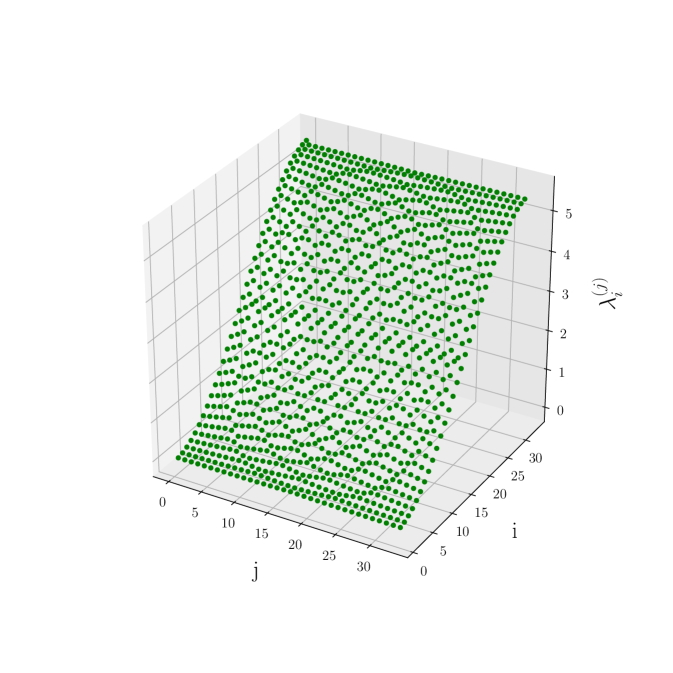
Of course, there is a drawback in the expression (1) and it is the requirement of the calculation of the eigenvalues for different matrices, which, in general, takes more computational efforts than the direct diagonalization of an matrix. The algorithm can be improved significantly if one can found some relationship between the original eigenvalues and the corresponding minor eigenvalues . To this end, we first plot these eigenvalues, to see if they follow some identifiable behavior. We show, in Figure 1, the values corresponding to an infinite potential well (Eq. (6)) of size a.u. and amplitude , calculated with a numerical grid having points. From this figure, we can not get any useful information, because of the similarities among the eigenvalues, for any minor matrix .
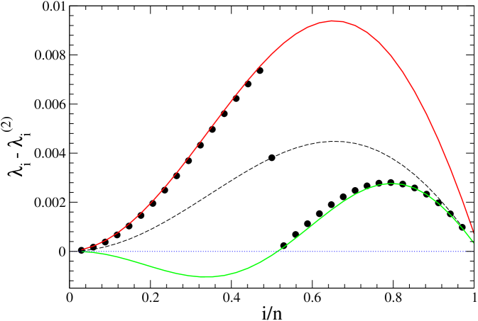
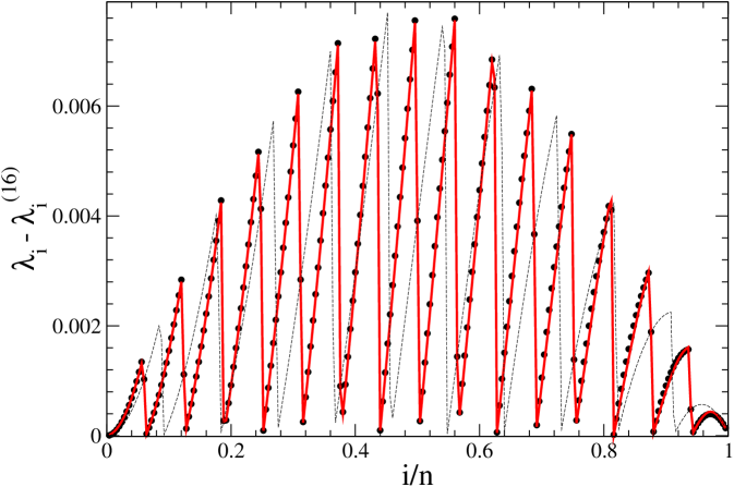
For a better representation, we define and plot, in Figure 2 the differences , which could be helpful to understand the meaning of the minor’s eigenvalues.
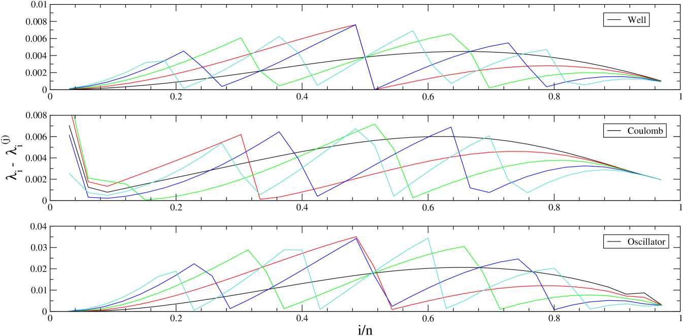
These differences have been calculated for three different potentials, an infinite potential well, a Coulomb potential, and a harmonic oscillator potential. An unexpected regular pattern appears in the three cases, encouraging the search for analytical expressions capable to represent these values.
III Analytical expression for the minor’s eigenvalues
Although the curves shown in Fig. 2 suggest the possibility to find analytical functions to represent the minor’s eigenvalues, this task is not straightforward. Let us analyze the eigenvalues of the minor matrices for the infinite potential well , which seems to be the potential having the most regular behavior. It is important to stress that we are dealing with the numerical solutions of a first order finite–differences approximation, which are different than the exact solutions. We will first attempt to understand the state of affairs in the numerical solutions, and will treat the exact solutions in further works (see a brief discussion in Appendix B).
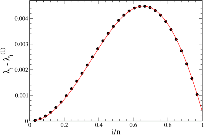
For the first minor matrix , the differences are arranged in a smooth curve which is easily approximated, as is shown in Figure 3, by the expression
| (7) |
where is very close to , the number of points in the numerical grid.
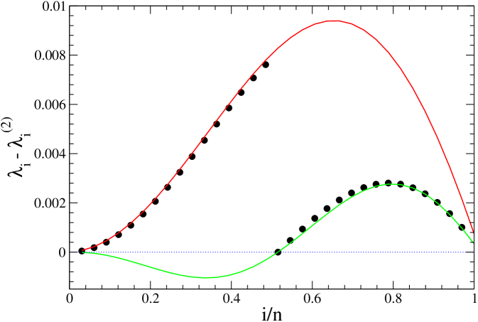
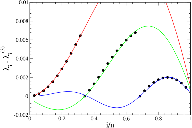
The analytic approximation is more difficult for the next minor matrix . Here, there are two different noticeable regions , and each one should be approximated separately, i.e.,
| (8) |
For the first coefficient , but, for the second half of the eigenvalues (), the appropriate value is (formal expressions for are given in Appendix A).
The complications related to pursuing an understanding of the behavior of the minor’s eigenvalues do not end here. We found that the size of the Hamiltonian also affects how the are approximated. Let see these values for a case in which the number of points in the numerical grid is even. Figure 5 shows the differences between the eigenvalues of a Hamiltonian matrix with points (in place of the previous values showed in Fig. 4, where ).
Here, the differences for the first 16 eigenvalues are approximated with (8) using a set of parameters and , and the last 16 by using another set, like in the previous case. But, the difference does not belong to either of both curves. Surprisingly, we found that this value agrees exactly with the difference got for the first minor, which is .
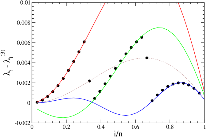
More intricate is the approximation for the minor’s eigenvalues (). We start the analysis with a Hamiltonian matrix having points. As is shown in Figure 6, we need to establish three different regions , where the size of each one is pretty near (see Appendix A). Since 34 is not divisible by 3, we do not know beforehand how many points belong to each region .
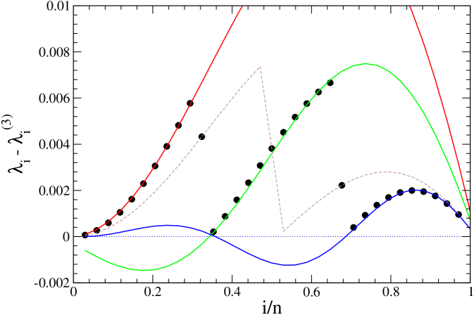
We found that the approximation (8) works well for the three ranges if considering 11 points belonging to the first and last regions and 12 points to the middle. The corresponding parameters are roughly , , . As pointed out before, this distribution is particular for a given Hamiltonian size. The –case is illustrated in Figure 7. Here, 10 eigenvectors can be fitted very well with (8), for each region . We run into troubles at two points corresponding to and . As shown in the figure, the same unexpected property found before holds for this case: for these points, the eigenvalue differences for coincide exactly with the corresponding values of the first minor .
Nevertheless, the picture is different for , as is shown in Figure 8. Here, the first and last region holds 10 points, the central region 11 points, and, again, two values lie outside these curves. Now, these values agree exactly with those corresponding to .
In conclusion, the eigenvalue differences follow the general behavior given in Eq.(8), in which the width coefficients
| (9) |
But, it seems very difficult to assign a simple formula for each minor index , for each region , and for any number of points .
We emphasize that the expression (9) is approximate. An accurate fitting for the values can be done, requiring a lot of work since adjustments must be done to generalize it for every number of points . These corrections are small and will not be significant for large matrices. However, establishing the number of points assigned to each sector is not straightforward since it depends on the number of points and varies for each minor index . Assigning a wrong number of points to a particular region accumulates enormous errors in the reconstruction formula (1), turning any approximation of useless. Furthermore, there are many problematic points , that do not belong to any of the regions . The differences for these points agree with the values calculated for other minors , where the minor index also depends on and the number of points . We found the analytical expression that relates these indexes:
| (10) |
Taking all these aspects into consideration, we can reproduce all the values, and thus, all the eigenvalues belonging to all the minor matrices , for any Hamiltonian size . As an example, we illustrate, in Figure 9, the eigenvalue differences for the minor matrix , for a Hamiltonian matrix with points. All the points that are not fitted with the curves represented in solid lines have exactly the values corresponding to the minor matrix (dashed curves), in agreement with our findings, since .
IV Physical interpretation of the minor’s eigenvalues
Having decoded the startling pattern conformed by the minor’s eigenvalues, many questions remain open. The behavior discovered is particular to the infinite potential well. From Figure 2 it is reasonable to conjecture about the existence of similar relationships on the other potentials. All the eigenvalues have been calculated numerically. A question arises is whether the same pattern holds also for the exact analytical results. The most important issue to solve is the possibility to recognize a physical meaning in our findings. Perhaps, understanding this matter could help to answer the other questions.
The first physical realization of the eigenvector–eigenvalue identity has been done by Voss and Balloon Voss:20 . They showed that one–dimensional arrays of coupled resonators, described by square matrices with real eigenvalues, provide simple physical systems where this formula can be applied in practice. The subsystems consist of arrays with the resonator removed. Thus, from their spectra alone, the oscillation modes of the full system can be obtained.
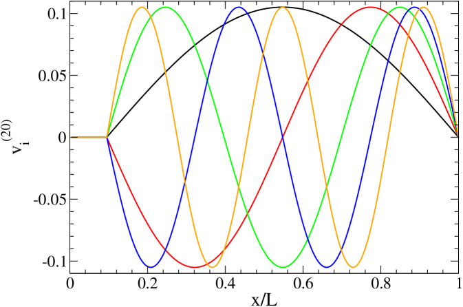
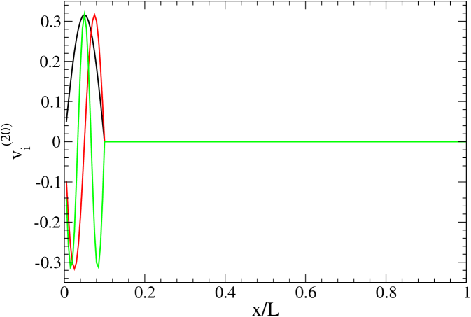
Concerning the infinite potential well, the physical meaning of the removal of the first row and column is very simple: it conforms another infinite potential well whose width decreases from to , where is the numerical mesh size. The same potential may be thought of as an infinite well of size , with an additional infinite wall located at . Accordingly, the removal of the row and column means an infinite potential well with an infinite wall at . As an example, we plot the first eigenvectors of the submatrix , for an infinite potential well represented by points, in Figure 10 (above). In the relative coordinates it means that an infinite wall is present at . As is shown in the figure the first eigenvectors correspond to the eigenvectors of a infinite potential well. We also have to consider the other potential well of size , which, for this particular case have eigenvalues coincident with the full Hamiltonian spectra for every functions. The lower part of Figure 10 shows the eigenvalues , , and , having the same energy as , , and from the full Hamiltonian.
V Conclusions
The eigenvalue–eigenvector identity expresses a curious and surprising relationship between the eigenvector of a matrix and the eigenvalues of its minors. It can be very useful from the numerical point of view, encouraging the study of new techniques to solve large eigenproblems. In general, it is much simple and fast to calculate the eigenvalues than the eigenvectors. Moreover, for very large matrices, the memory storage requirement for standard eigenvectors solver can lead to serious problems, which could be overcome by this approach. A critical element to strengthening the use of the identity is the ability to avoid the calculation of the eigenvalues of all the minor matrices.
In this work, we first tested the eigenvalue–eigenvector identity on different systems. The formula has been used to reconstruct, numerically, the eigenvectors of simple one–dimensional Hamiltonians. Using only the eigenvalues of the minor matrices, the formula reproduces the eigenvectors within machine precision, even for large cases. In most cases, the eigenvalue is close to the value. However, analyzing their differences , we found systematic patterns, allowing to extract analytically the minor’s eigenvectors without diagonalizing all the submatrices.
To understand the patterns, we focused our study on the infinite potential well. Elucidating the behavior of the differences is not straightforward since they depend on the eigenvalue index , the minor index , and also on the number of points in the numerical grid representing the Hamiltonian. We found that, indeed, it is possible to find an analytical expression for , and therefore, for all the . The existence of regular patterns suggest that some hidden information about the eigenvectors of the full Hamiltonian is buried under the minor matrices’ eigenvalues structure. A crucial aspect to understand this information is to found the physical reasons that generate those patterns. For the case studied here, the minor matrix represents a clear physical case that consists of the same Hamiltonian but with an infinite wall located at the point corresponding to the index . The generalization to other potentials in 3 dimensions and for real scenarios, can be a matter of further interesting development.
Acknowledgements.
This work was supported with PIP N of CONICET, Argentina.The data that support the findings of this study are available from the corresponding author upon reasonable request.
References
- (1) P.B. Denton, S.J. Parke and Xining Zhang, “Eigenvalues: the Rosetta Stone for Neutrino Oscillations in Matter”, arXiv:1907.02534 [hep–ph], (2019).
- (2) P.B. Denton, S.J. Parke, T. Tao, and Xining Zhang, “Eigenvectors from Eigenvalues: a survey of a basic identity in linear algebra”, arXiv:1908.03795 [math.RA], (2019).
- (3) N. Wolcholver, “Neutrinos lead to unexpected discovery in basic math”, Quanta Magazine, Nov (2019), http://shorturl.at/bcqsA.
- (4) LAPACK: Linear Algebra PACKage, http://www.netlib.org/lapack/.
- (5) H.U. Voss and D.J. Ballon, Phys. Rev. Research 2 012054(R), (2020).
Appendix A Analytical expression for the approximation formulas
In first–order approximation, the numerical eigenvalues of the one dimension infinite potential well, are related to the eigenvalues of the minor submatrix in the following way. Let us define a variable
| (11) |
where is the eigenvalue index and is the number of grid points representing the eigenvectors. Numerically, an infinite potential well represented by an –points Hamiltonian has different eigenvalues, therefore, . The eigenvalue differences have been found to cluster in different sections, where the size of each of them is approximately . More precisely, each section begins at a point
| (12) |
It is worth to note that for the infinite potential well, the points correspond to the nodes of the eigenvector.
The argument of the functions in Eq. (8) has a wavelength proportional to a width of
| (13) |
The differences can be approximated by the expression
| (14) |
The parameter
| (15) |
and the coefficients , , and in any other case
| (16) |
It is very important to identify the limits of every sector : the initial eigenvalue index , the last point , and the points that lie outside each region . For simplicity, let us drop the indexes and in Eq. (12), so, every section is bounded by the range
| (17) |
The corresponding values are not necessarily integer numbers. We define the indexes and as the integer part of and , respectively. Then, we designate the following quantities:
| (18) |
The index is defined as
| (19) |
Every sector contains the eigenvalue indexes between
| (20) |
As explained above, the value of is calculated by using Eq. (10), i.e., the value corresponding to the index is where
| (21) |
Appendix B Implementation in the exact solutions
Here, we will show how to proceed for the reconstruction of the exact wavefunctions (not the numerical solutions, as before). Again, we want to get the eigenvectors of an infinite potential well, using the eigenvector–eigenvalue identity. The expression (1) involves a product, so, we must decide, first, how many points should be used in it. This decision also determines which minor matrices are included, and their eigenvalues. As stated above, the minor matrix represents the original Hamiltonian matrix with an infinite wall at the corresponding position . This wall separates the potential in two regions, in our case, two infinite wells, one from 0 to , and the other from to . To reconstruct the eigenvectors through the eigenvector–eigenvalue identity, one must be aware to intercalate appropriately the energies of both wells.
As an example, let us pick 10 terms in the product (1) to reconstruct the eigenvectors of an infinite potential well having a width a.u.. The walls are located at a.u.. For instance, for the minor , we need to calculate the spectra for two wells: one having a width and the other with . Their corresponding energies are
| (22) |
For the box having a.u., the lowest energies are , , and a.u., and for a.u., the lowest energies are , , and a.u.. The ordered eigenvalues are stated in Table LABEL:tab:eigenvalues, together with the other values. The rest of the eigenvalues are got by considering the symmetry of the potentials, i.e., , , , , and .
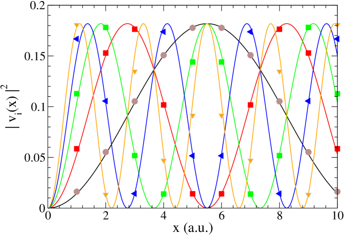
Using these eigenvalues, the eigenvector–eigenvalue equation reproduces the eigenvectors (at the positions ), without normalization. The normalized results are shown in Figure 11, for the first five eigenvalues, demonstrating that the identity can also be used for exact analytical cases.
| H | 0.0408 (11,1) | 0.1631 (11,2) | 0.3671 (11,3) | 0.6525 (11,4) | 1.0196 (11,5) | 1.4682 (11,6) | 1.9984 (11,7) | 2.6101 (11,8) | 3.3035 (11,9) |
|---|---|---|---|---|---|---|---|---|---|
| 0.0493 (9,1) | 0.1974 (9,2) | 0.4441 (9,3) | 0.7896 (9,4) | 1.2337 (2,1) | 1.7765 (9,5) | 2.4181 (9,6) | 3.1583 (9,7) | 3.9972 (9,8) | |
| 0.0609 (8,1) | 0.2437 (8,2) | 0.5483 (3,1) | 0.9748 (8,3) | 1.2337 (8,4) | 1.5231 (8,5) | 2.1932 (3,2) | 2.9853 (8,6) | 3.8991 (8,7) | |
| 0.1007 (7,1) | 0.3084 (4,1) | 0.4028 (7,2) | 0.9064 (7,3) | 1.2337 (4,2) | 1.6114 (7,4) | 2.5178 (7,5) | 2.7758 (4,3) | 3.6256 (7,6) | |
| 0.1371 (6,1) | 0.1974 (5,1) | 0.5483 (6,2) | 0.7896 (5,2) | 1.2337 (6,3) | 1.7765 (5,3) | 2.1932 (6,4) | 3.1583 (5,4) | 3.4269 (6,5) |