Wavelet Based Periodic Autoregressive Moving Average Models

Time series with seasonal or periodic patterns occur in many fields of applications such as economics, finance, demography, astronomy, meteorology, etc. The commonly used seasonal autoregressive integrated moving average (SARIMA) models may not capture some of the important local features of such time series (see [14]). An alternative approach suggested is to model these data by periodically stationary time series. A process $\{\tilde{Y}_{t}\}$ is said to be periodically (weak) stationary if mean function $\mu_{t}=E(\tilde{Y}_{t})$ and autocovariance function $\gamma_{t}(h)=Cov(\tilde{Y}_{t},\tilde{Y}_{t+h}),h\in\mathbb{Z}$, are periodic functions with same period $\nu$ (see [20]). A particular class of models having periodic stationarity is the periodic autoregressive moving average models of period $\nu$ having autoregressive parameter $p$ and moving average parameter $q$ [$\text{PARMA}_{\nu}(p,q)$], given in [6] is

where (i) $Y_{t}=\tilde{Y}_{t}-\mu_{t},\mu_{t}=\mu_{t+k\nu},k\in\mathbb{Z},$ (ii) $\phi_{t}=\phi_{t+k\nu},k\in\mathbb{Z}$, (iii) $\theta_{t}=\theta_{t+k\nu},k\in\mathbb{Z}$, and (iv) $\sigma^{2}_{t}=\sigma^{2}_{t+k\nu},k\in\mathbb{Z}$, where $\sigma^{2}_{t}$ is the variance of the mean zero random sequence $\{\varepsilon_{t}\}$. Thus, $\{\delta_{t}\}=\{\sigma_{t}^{-1}\varepsilon_{t}\}$ is an iid sequence of mean 0 and variance 1 random variables. Note that PARMA reduces to ARMA when $\nu=1$. PARMA models have been applied in fields as diverse as economics ([21] and [9]), climatology ([13], [7] and [4]), signal processing [10] and hydrology ([25], [24], [6], [1] and [5]). However, PARMA models contain a large number of parameters. For example, for a monthly series of period $\nu=12$, the total number of parameters to be estimated is $12\times 4=48$. Often, the inclusion of a large number of parameters leads to overfitting. Hence, it is important to develop methods that result in parsimonious models having less number of parameters.

This article is organised in the following manner: In Section 2, the estimators of the PARMA model and their several properties are mentioned. The Fourier-PARMA model is presented in Section 3. Section 4 gives a brief introduction to wavelet analysis with a special focus on discrete wavelet transform. In Section 5, our proposed wavelet-PARMA model is expounded. Section 6 consists of a simulation study of our proposed wavelet-PARMA model. The applicability of the proposed model is demonstrated using real data in Section 7. Section 8 contains the conclusion of our study. We have utilised the results from various articles, and for easy reference, we have included them in the Appendices.

It is assumed hereafter that model (1) admits a causal representation (see [4])

where $\psi_{t}(0)=1$ and $\sum_{j=0}^{\infty}\left|\psi_{t}(j)\right|<\infty,$ for all $t$. Note that $\psi_{t}(j)=\psi_{t+kv}(j)$ for all $j$. Also, $Y_{t}=\tilde{Y}_{t}-\mu_{t}$ and $\varepsilon_{t}=\sigma_{t}\delta_{t}$ where $\left\{\delta_{t}\right\}$ is i.i.d.

Given data $\tilde{Y}_{0},\tilde{Y}_{1},\dotsc,\tilde{Y}_{N\nu-1}$, where $N$ is the number of cycles, the vector $\boldsymbol{\mu}=\{\mu_{0},\dotsc,\mu_{\nu-1}\}^{\prime}$ is estimated using

The sample autocovariance for lag $m$ and season $i$ is estimated using

where $\hat{\mu}_{i}$ is estimated using (2) and whenever $t>N\nu-1$, the corresponding term is set as zero. Let

denote the one-step predictor of $Y_{i+n}$ that minimises the mean square error, $v_{n,i}=E(Y_{i+n}-\hat{Y}_{i+n})^{2}$. The estimates of $\theta_{n,j}^{(i)}$ and $v_{n,i}$ can be obtained by substituting the estimates of autocovariance function (3) in the recursive relation of innovation algorithm for periodic stationary processes given in Theorem A1. Then, Theorem A2 and Theorem A3 show that $\hat{\theta}_{n,j}^{\langle i-n\rangle}$ and $\hat{v}_{n,\langle i-n\rangle}$ are consistent estimators for $\psi_{i}(j),$ for all $j$, and $\sigma_{i}^{2}$ respectively. Here the notation, $\langle b\rangle$ is $b-\nu\lfloor b/{\nu}\rfloor\,\text{for}\,b=0,1,\dotsc$ and $\nu+b-\nu\lfloor b/{\nu}+1\rfloor$ for $b=-1,-2,\dotsc$, where $\lfloor\cdot\rfloor$ is the greatest integer function.

To demonstrate our proposed ideas we are focusing particularly on two classes of PARMA models, described in the following subsections.

Often, it is found that representing a function in terms of basis terms helps us to get new insights about the function, which is otherwise obscure. The selection of the set of basis functions depends on the kind of information we are interested in. The analysis of periodic functions usually involves the identification of prominent frequencies present in the signal. For this the function is represented as an infinite series of sinusoids, known as Fourier series, which is possible for almost all functions encountered in practice. The magnitude of the coefficients associated with sines and cosines indicates the strength of the corresponding frequency component present in the process.

For a given vector $\mathbf{X}$, from [4], the periodic function $\mathbf{X}=[X_{t}:0\leq t\leq\nu-1]$ has the representation

where $c_{r}$ and $s_{r}$ are Fourier coefficients and

For convenience, (8) is written as,

where $cos^{*}(r)=cos\left(\frac{2\pi rt}{\nu}\right)$ and $sin^{*}(r)=sin\left(\frac{2\pi rt}{\nu}\right)$.

Let $\textbf{f}=\begin{cases}[c_{0},c_{1},s_{1},\dotsc,c_{(\nu-1)/2},s_{(\nu-1)/2}]^{\prime}\quad(\nu\,\text{odd})\\ [c_{0},c_{1},s_{1},\dotsc,s_{(\nu/2-1)},c_{(\nu/2)}]^{\prime}\quad\quad(\nu\,\text{even})\end{cases}$.

Then, we have, from [4],

where $\mathcal{L},\mathcal{P}$ and $\mathcal{U}$ are respectively given in equations (60), (62) and (61) of Theorem A11. $\mathcal{U}$ and $\mathcal{P}$ are unitary matrices. Using (10), we have, $\hat{\textbf{f}}=\mathcal{L}\mathcal{P}\mathcal{U}\hat{\mathbf{X}}$. Note that X can be retrieved from f by,

where $\tilde{\mathcal{A}}^{\prime}$ denotes the conjugate transpose of matrix $\mathcal{A}$. Thus, X and f are representations of the same entity. Hence, to obtain a parsimonious PARMA model it is enough to represent the model using a reduced number of Fourier coefficients. Since it is observed that PARMA parameters often vary smoothly over time, [6], [5], [23] and [4] identified significant Fourier coefficients via a hypothesis test based on the asymptotic distributions of PARMA estimators. The significant Fourier coefficients are retained as it is while the insignificant coefficients are reduced to zero, thereby resulting in a parsimonious Fourier-PARMA model.

Although some success has been found in employing Fourier techniques they often fail when bursts and other transient events take place, which is often the case in many fields like economics and climatology. This is because, in the case of temporal events, all the Fourier coefficients get unduly affected as all the observations are involved in the computation of the coefficients.

Wavelet techniques are an excellent alternative to Fourier methods. Some applications of wavelets in statistics include estimation of functions like density, regression, and spectrum, analysis of long memory process, data compression, decorrelation, and detection of structural breaks. A “wavelet” means small wave (see [22], [18] and [11]). This essentially means that a wavelet has oscillations like a wave. However, it lasts only for a short duration unlike sine wave, which spans infinitely to both sides of the time axis. They are constructed so that they possess certain desirable properties. Many different wavelet functions and transforms are available in the literature. However, here we are considering only the orthogonal discrete wavelet transform (DWT) since the approximation based on an orthogonal set is best in terms of mean square error, as indicated by projection theorem (see [8]).

Fourier methods are enough when the frequencies of the signal do not change over time. However, Fourier techniques fail when different frequencies occur at different parts of the time axis. Hence, it is imperative to find techniques that have both time resolution and frequency resolution. But, by Heisenberg’s Principle, it is impossible to identify time and frequency simultaneously with arbitrary precision (see [15] and [26]) as there is a lower bound for the error occurred. However, wavelets intelligently bypass this difficulty by using short time windows to capture high frequency, so that we have good time resolution, and wider time windows for low frequencies so that we have good frequency resolution. Thus, wavelets can pick out characteristics that are local in time and frequency. Wavelets are functions of scale, instead of frequency. A scale can be loosely interpreted as a quantity inversely proportional to frequency. This makes the wavelet transform an exceptional tool for studying non-stationary signals. For the latest works on the applications of wavelets to time series, one can refer to [16], [27], and [17].

Let $\mathbf{X}$ be a vector of size $N=2^{J},J\,\in\,\mathbb{Z}^{+}$, $\mathcal{W}$ is an $N\times N$ orthogonal matrix used for performing discrete wavelet transform (DWT), then the DWT of $\mathbf{X}$ is given by,

Here, ${V}_{J}=W_{0}$, is the scaling coefficient that is proportional to the average of all the data, i.e,

where the proportionality constant $k_{1}$ depends on the particular wavelet employed. $\mathbf{W}_{j},j\in\{1,2,\dotsc,J\}$ contains $2^{j-1}$ wavelet coefficients associated with changes on a scale $N/2^{j-1}$. For example, the Haar DWT of $\mathbf{X}=[X_{0},\dotsc,X_{15}]^{\prime}$ is given by,

Note that the wavelet coefficients are localised in time. For example, the last wavelet coefficient only involves the observations $X_{14}$ and $X_{15}$. Since $\mathcal{W}$ is an orthogonal matrix, the original vector $\mathbf{X}$ can easily be reconstructed via the inverse DWT

where $\mathcal{W}^{T}$ denotes the transpose of $\mathcal{W}$. Note that from (14), X and W are representations of the same quantity and hence it is enough to represent the parameters of the PARMA model in terms of discrete wavelet transform coefficients.

Another interesting advantage of the DWT, especially pertaining to our objective of achieving parsimonious PARMA models, is the fact that DWT redistributes the energy or variability contained in a sequence (see [26]). Hence, the crux of the sequence, spread throughout the original sequence, is concentrated in a few wavelet coefficients (see [19] and [26]). Hence, we propose a wavelet-PARMA model that captures the dependency structure adequately based on the idea of retaining only a few significant wavelet coefficients. We identify the significant wavelet coefficients by developing a hypothesis test, following the parallel approach given in [4] for Fourier coefficients, utilizing the asymptotic distributions of the estimators of the PARMA parameters.

Suppose random vector $\hat{\mathbf{X}}$ satisfies,

Using Theorem A12, we have,

The main idea is to identify the statistically significant wavelet coefficients of the PARMA estimator vectors, using an appropriate test procedure so that the other coefficients can be nullified, thereby obtaining a parsimonious PARMA model. The null hypothesis of the test is $H_{0}:\mathbf{W}=(V_{J},0,\dotsc,0)=(W_{0},0,\dotsc,0)$. Under $H_{0}$, $\mathbf{X}=k_{2}*V_{J}=k_{2}*k_{1}*\frac{1}{N}\sum_{i=1}^{N}X_{i}=k*\frac{1}{N}\sum_{i=1}^{N}X_{i}$, where $k$ depends on the type of wavelet used. Since the parameter vectors have all elements the same under $H_{0}$, the PARMA process reduces to a stationary ARMA process with $\phi_{t}=\phi$ for all $t\in\{0,1,\dotsc,\nu-1\}$, and similarly for other parameter vectors. Thus, the null hypothesis states that the model is stationary. From (16), we have,

Here, we will use the Bonferroni’s test procedure (see [12]) with $\alpha=0.05$. In this case, we wish to test the null hypothesis $H_{0}:|W_{i}|=0$ versus $H_{a}:|W_{i}|\neq 0,i=1,2,\dotsc,\nu-1$. The test statistics is

Let $\alpha^{*}=\frac{\alpha}{\nu-1}$ and $Z_{\alpha^{*}/2}$ be the $\alpha^{*}/2$ tail quantile, i.e, $P(|Z|>Z_{\alpha^{*}/2})=\alpha^{*}/2$, where $Z\sim\mathcal{N}(0,1)$. We reject the null hypothesis when $|{Z_{W}}_{i}|>Z_{{\alpha^{*}}/2}$. Whenever the null hypothesis is not rejected, the corresponding element $W_{i}$ is set as zero. Hopefully, this will result in a sparse $\mathbf{W}^{\prime}$ vector where most of the coefficients are 0, resulting in a parsimonious wavelet-PARMA model.

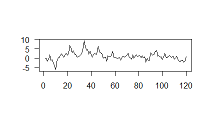
The observations are simulated from the $\text{PARMA}_{12}(1,1)$ model,

where (i) $\phi_{t}=\phi_{t+12k}$, (ii) $\theta_{t}=\theta_{t+12k},k\in\mathbb{Z}$ and $\{\varepsilon_{t}\}$ is a sequence of normal random variables with mean 0 and variance 1. The parameter values and their corresponding estimates are given in Table 6.

Since period 12 is not a power of 2, each of the vectors has been extended periodically to the nearest power of 2, i.e, 16. We have taken the number of cycles, $N$ to be 500.

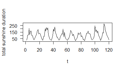
The plot of the generated observations is given in Figure 1.

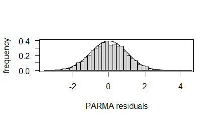
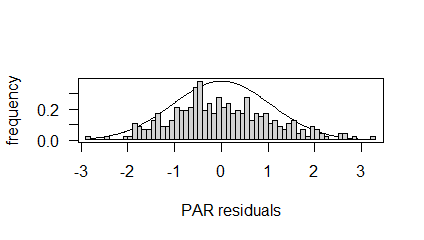
7 iterations of the innovation algorithm was carried out to calculate the parameter estimates. The residuals are computed using the expression,

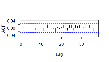
where the initial value $\hat{\varepsilon}_{0}$ is set as zero. The residual diagnostic plots are given in Figure 2.

The Box Pierce test results are given in Table 6.

The normality of the residuals was tested using Kolmogorov Smirnov test and it was found that the residuals are normally distributed (p-value = 0.8586). Thus, the residuals are uncorrelated and normally distributed.

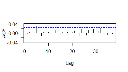
The obtained Fourier-PARMA model, by using the method outlined in [4] is given by,

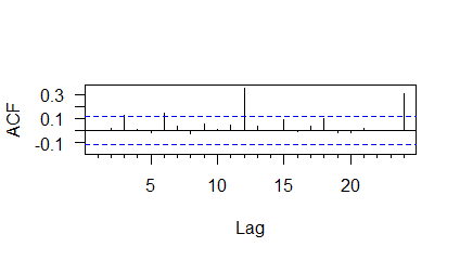
The ACF plot of residuals of the Fourier-PARMA model is given in Figure 3.

The results of Box-Pierce test are given in Table 6.

Thus, the Fourier-PARMA model is not able to capture the dependencies among the observations adequately as is evident from the ACF plot given in Figure 3 and Box-Pierce test results given in Table 6.

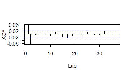
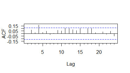
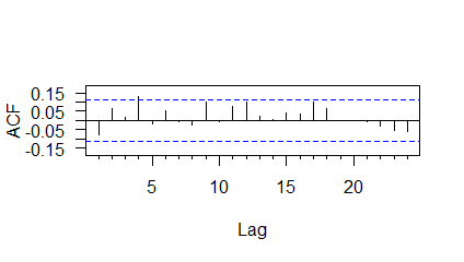
The discrete wavelet transform analysis was done using Haar wavelet. This wavelet was chosen for simulation because its structure is explicitly known. The results of Haar DWT analysis are given in Table 6. It is found that only 4 DWT coefficients of $\phi$ and 4 DWT coefficients of $\theta$ need to be incorporated into the wavelet-PAR model and so the final model contains only 8 parameters as opposed to 24 parameters in the original PARMA model. The ACF plot of the residuals of wavelet-PARMA model is given in Figure 4.

The results of Box-Pierce test are given in Table 6.

The residuals of the wavelet-PARMA model are uncorrelated. Hence, the wavelet-PARMA model with just 8 parameters is able to capture the dependency structure adequately.

The UK Meteorological (MET) Office, established in 1854, is the government body commissioned to analyse weather in the United Kingdom. They use their findings for forecasting and for issuing warnings. They offer data from 36 stations in the UK. For our analysis, we have considered the total sunshine duration in a month recorded in hours by the Ballypatrick weather station for the years 1966-1990. This data is available from the Kaggle site https://www.kaggle.com/datasets/josephw20/uk-met-office-weather-data/code, where the total sunshine duration is given under the variable sun. The data considered is fit using the $\text{PAR}_{12}(1)$ model given in equation (4). Here, period $\nu=12$ and the number of years (cycles), $N=25$. The plot of the first 10 years is given in Figure 5. It was found that 2 iterations of the innovation algorithm were enough to capture the model dynamics. The residuals of the PAR model was computed using,

where $\hat{Y}_{t}=\tilde{Y}_{t}-\hat{\mu}_{t}$. The PAR model diagnostics plots are given in Figure 6. The results of the Box-Pierce test are given in Table 7. The normality of the residuals was tested using the Kolmogorov-Smirnov test and it was found that the residuals were normally distributed (p-value = 0.319). Thus, the residuals are uncorrelated and normally distributed.

The obtained Fourier-PAR model, by using the method outlined in [4] is given by,

The ACF plot of Fourier-PAR residuals is given in Figure 7.

The results of Box-Pierce test of Fourier-PAR residuals are given in Table 7.

Thus, it is clear that the Fourier-PAR model has not been able to capture the dependency structure adequately.

The discrete wavelet transform analysis was done using Daubechies least asymmetric wavelet with 7 vanishing moments. This wavelet was chosen because the resulting wavelet-PAR model could capture the dependency structure adequately. The LA(7) DWT results are given in Table 7. The ACF plot of wavelet-PAR residuals is given in Figure 8. The Box-Pierce test of wavelet-PAR residuals is given in Table 7. From these results, it is clear that the resulting wavelet-PAR model was able to capture the dependency structure adequately. It is found that only 7 DWT coefficients of $\boldsymbol{\mu}$, 1 DWT coefficient of $\boldsymbol{\phi}$, and 5 DWT coefficients of $\boldsymbol{\sigma^{2}}$ need to be incorporated into the wavelet-PAR model and so the final model contains only 13 parameters as opposed to 36 parameters in the original PAR model.

PARMA models are used extensively in various fields like economics, climatology, signal processing and hydrology. However, the presence of a substantial number of parameters in a PARMA model reduces its efficiency. Fourier methods already exist in the literature for reducing the number of parameters and have found some success when the parameters vary slowly. However, transient events are quite common in real-life applications and wavelet techniques stand out as the principal analysis tool in these situations. The efficiency of wavelet methods in reducing the number of parameters of PARMA models has been demonstrated using a simulation study and their applicability in real life has been illustrated using real data. This study opens new avenues for the reduction of parameters in other classes of models containing a large number of parameters.

Rhea Davis acknowledges the financial support of the University Grants Commission (UGC), India under the Savitribai Jyotirao Phule Fellowship for Single Girl Child (SJSGC) scheme.

There is no conflict of interest between the authors.

In this section, we state the results used to analyse our models, which were proved under the following assumptions:

Let $\{Y_{t}\}$ be a process defined by (1). Then,

1. B1.

   Finite Fourth moment: $E\varepsilon_{t}^{4}=\eta<\infty$.

2. B2.

   The model admits a causal representation

   $$Y_{t}=\sum_{j=0}^{\infty}\psi_{t}(j)\varepsilon_{t-j},$$

   where $\psi_{t}(0)=1$ and $\sum_{j=0}^{\infty}\left|\psi_{t}(j)\right|<\infty$ for all $t$. Note that $\psi_{t}(j)=\psi_{t+k\nu}(j)$ for all $j$. Also, $Y_{t}=\tilde{Y}_{t}-\mu_{t}$ and $\varepsilon_{t}=\sigma_{t}\delta_{t}$, where $\{\delta_{t}\}$ is i.i.d.

3. B3.

   The model satisfies an invertibility condition

   $$\varepsilon_{t}=\sum_{j=0}^{\infty}\pi_{t}(j)Y_{t-j},$$

   where $\pi_{t}(0)=1$ and $\sum_{j=0}^{\infty}\left|\pi_{t}(j)\right|<\infty$ for all $t$. Again, $\pi_{t}(j)=\pi_{t+k\nu}(j)$ for all $j$.

4. B4.

   The spectral density matrix $f(\lambda)$ of the equivalent vector ARMA process given by,

   $$U_{t}=\sum_{j=-\infty}^{\infty}\Psi_{j}Z_{t-j},$$

   (40)

   where $U_{t}=(Y_{t\nu},\dotsc,Y_{(t+1)\nu-1})^{\prime}$, $Z_{t}=(\varepsilon_{t\nu},\dotsc,\varepsilon_{(t+1)\nu-1})^{\prime}$ and $\Psi_{t}$ is the $\nu\times\nu$ matrix with $ij$ entry $\psi_{i}(t\nu+i-j)$ and for some $0<c\leq C<\infty$ we have,

   $$cz^{\prime}z\leq z^{\prime}f(\lambda)z\leq Cz^{\prime}z,\quad-\pi\leq\lambda\leq\pi,$$

   for all $z$ in $R^{\nu}$.

5. B5.

   The number of iterations $n$ of the iterations algorithm satisfies $n\leq Nv-1$, and $n^{2}/N\rightarrow 0$ as $N\rightarrow\infty$ and $n\rightarrow\infty$.

6. B6.

   The number of iterations $n$ of the iterations algorithm satisfies $n\leq Nv-1$, and $n^{3}/N\rightarrow 0$ as $N\rightarrow\infty$ and $n\rightarrow\infty$.

References

- [1] P.L. Anderson and M.M. Meerschaert, Modeling river flows with heavy tails, Water Resources Research 34 (1998), pp. 2271–2280.
- [2] P.L. Anderson and M.M. Meerschaert, Parameter estimation for periodically stationary time series, Journal of Time Series Analysis 26 (2005), pp. 489–518.
- [3] P.L. Anderson, M.M. Meerschaert, and A.V. Vecchia, Innovations algorithm for periodically stationary time series, Stochastic Processes and their Applications 83 (1999), pp. 149–169.
- [4] P.L. Anderson, F. Sabzikar, and M.M. Meerschaert, Parsimonious time series modeling for high frequency climate data, Journal of Time Series Analysis 42 (2021), pp. 442–470.
- [5] P.L. Anderson, Y.G. Tesfaye, and M.M. Meerschaert, Fourier-parma models and their application to river flows, Journal of Hydrologic Engineering 12 (2007), pp. 462–472.
- [6] P. Anderson and A. Vecchia, Asymptotic results for periodic autoregressive moving-average processes, Journal of Time Series Analysis 14 (1993), pp. 1–18.
- [7] P. Bloomfield, H.L. Hurd, and R.B. Lund, Periodic correlation in stratospheric ozone data, Journal of Time Series Analysis 15 (1994), pp. 127–150.
- [8] P.J. Brockwell and R.A. Davis, Time series: theory and methods, Springer science & business media, 1991.
- [9] P.H. Franses and R. Paap, Periodic time series models, OUP Oxford, 2004.
- [10] W. Gardner and L. Franks, Characterization of cyclostationary random signal processes, IEEE Transactions on information theory 21 (1975), pp. 4–14.
- [11] W. Härdle, G. Kerkyacharian, D. Picard, and A. Tsybakov, Wavelets, approximation, and statistical applications, Vol. 129, Springer Science & Business Media, 2012.
- [12] D.C. Howell, Statistical methods for psychology, Cengage Learning, 2012.
- [13] R.H. Jones and W.M. Brelsford, Time series with periodic structure, Biometrika 54 (1967), pp. 403–408.
- [14] R. Lund and I. Basawa, Recursive prediction and likelihood evaluation for periodic arma models, Journal of Time Series Analysis 21 (2000), pp. 75–93.
- [15] S. Mallat, A wavelet tour of signal processing, Elsevier, 1999.
- [16] E.T. McGonigle, R. Killick, and M.A. Nunes, Trend locally stationary wavelet processes, Journal of Time Series Analysis 43 (2022), pp. 895–917.
- [17] H.A. Mohammadi, S. Ghofrani, and A. Nikseresht, Using empirical wavelet transform and high-order fuzzy cognitive maps for time series forecasting, Applied Soft Computing 135 (2023), p. 109990.
- [18] G.P. Nason, Wavelet methods in statistics with R, Springer, 2008.
- [19] R.T. Ogden, Essential wavelets for statistical applications and data analysis, Springer, 1997.
- [20] M. Pagano, On periodic and multiple autoregressions, The Annals of Statistics (1978), pp. 1310–1317.
- [21] E. Parzen and M. Pagano, An approach to modeling seasonally stationary time series, Journal of Econometrics 9 (1979), pp. 137–153.
- [22] D.B. Percival and A.T. Walden, Wavelet methods for time series analysis, Cambridge University Press, 2000.
- [23] Y.G. Tesfaye, P.L. Anderson, and M.M. Meerschaert, Asymptotic results for fourier-parma time series, Journal of Time Series Analysis 32 (2011), pp. 157–174.
- [24] A. Vecchia, Maximum likelihood estimation for periodic autoregressive moving average models, Technometrics (1985), pp. 375–384.
- [25] A. Vecchia, Periodic autoregressive-moving average (parma) modeling with applications to water resources 1, JAWRA Journal of the American Water Resources Association 21 (1985), pp. 721–730.
- [26] B. Vidakovic, Statistical modeling by wavelets, John Wiley & Sons, 1999.
- [27] J. Wang, S. Shao, Y. Bai, J. Deng, and Y. Lin, Multiscale wavelet graph autoencoder for multivariate time-series anomaly detection, IEEE Transactions on Instrumentation and Measurement 72 (2022), pp. 1–11.