Wavelet Canonical Coherence for Nonstationary Signals
Abstract
Understanding the evolving dependence between two clusters of multivariate signals is fundamental in neuroscience and other domains where sub-networks in a system interact dynamically over time. Despite the growing interest in multivariate time series analysis, existing methods for between-clusters dependence typically rely on the assumption of stationarity and lack the temporal resolution to capture transient, frequency-specific interactions. To overcome this limitation, we propose scale-specific wavelet canonical coherence (WaveCanCoh), a novel framework that extends canonical coherence analysis to the nonstationary setting by leveraging the multivariate locally stationary wavelet model. The proposed WaveCanCoh enables the estimation of time-varying canonical coherence between clusters, providing interpretable insight into scale-specific time-varying interactions between clusters. Through extensive simulation studies, we demonstrate that WaveCanCoh accurately recovers true coherence structures under both locally stationary and general nonstationary conditions. Application to local field potential (LFP) activity data recorded from the hippocampus reveals distinct dynamic coherence patterns between correct and incorrect memory-guided decisions, illustrating the capacity of the method to detect behaviorally relevant neural coordination. These results highlight WaveCanCoh as a flexible and principled tool for modeling complex cross-group dependencies in nonstationary multivariate systems. The code for WaveCanCoh is available at: https://github.com/mhaibo/WaveCanCoh.git.
1 Introduction
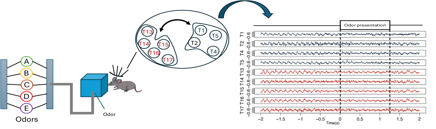
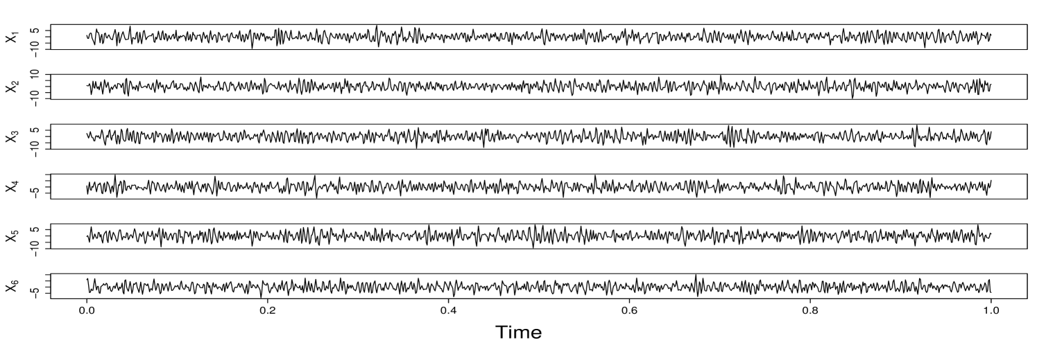
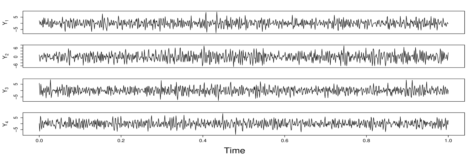
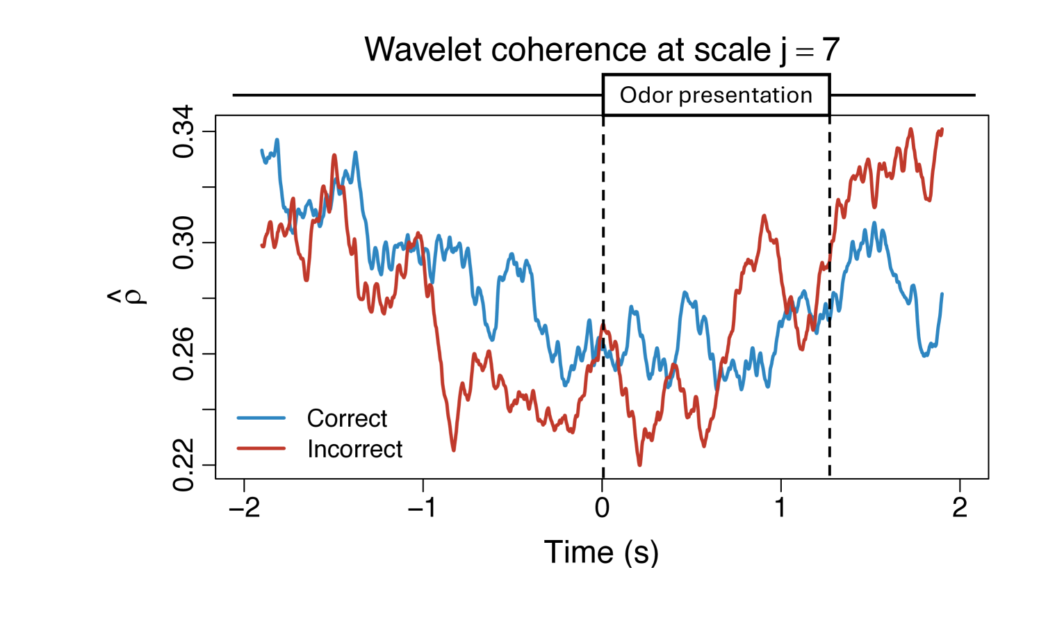
Assessing the dependence structure between node clusters in a network is one of the most critical aspects of network time series analysis. Many models and frameworks have been developed to capture between-clusters association (e.g., correlation, coherence, and causality). Most existing methods characterize the dependence between two clusters through the dependence between (many) node pairs. However, in many scenarios, the primary interest lies in understanding the dependence structure between two groups of multivariate time series rather than individual processes. Figure 1 illustrates this perspective using brain activity signals. In this experiment, local field potential (LFP) activity was recorded from multiple electrodes implanted in different subregions of the hippocampus of rodents (rats) as they performed a complex sequence memory task. Instead of focusing on coherence between individual channels (electrodes), the main goal is to quantify time-varying functional interactions between groups of electrodes in order to understand how information processing differs in these two subregions. Similar challenges arise in other domains. For instance, in finance, understanding the dependence between entire market sectors (e.g., technology and energy) can be more informative than analyzing associations between individual stocks. These scenarios require a framework capable of capturing dynamic coherence between sets of nonstationary multivariate signals. In this paper, we propose a novel framework called scale-specific wavelet canonical coherence (WaveCanCoh) to characterize time-localized and scale-specific coherence between two clusters of multivariate time series. By leveraging the time-frequency localization properties of wavelets, WaveCanCoh is well-suited for analyzing nonstationary multivariate signals in neuroscience, finance, and other fields where transient, cross-group interactions are of scientific interest.
Canonical variate analysis (CVA) (Hotelling (1936)) provides a method for measuring the correlation between two vector variables, its application to time series data having started in the 1950s and 1960s, primarily in the econometrics and signal processing fields. Box and Tiao (1977) and Geweke (1982) extend CVA to time series for forecasting and causality detection. Brillinger (2001) provides a spectral domain formulation of canonical correlation, useful for frequency-domain time series analysis. This approach enables the analysis of canonical coherence between two sets of time series across different frequency bands. Many modern studies have been developed within this framework (e.g., Talento et al. (2024) and Viduarre et al. (2019)), and related methods have been widely applied across various fields, including neuroscience, finance, speech processing, and machine learning.
However, previous methods rely on the assumption that time series are (weakly) stationary, meaning their statistical properties (e.g., expectation and covariance, spectral signature) remain constant over time. In practice, this assumption often does not hold for time series that arise in practice. Moreover, two sets of time series commonly exhibit time-varying global coherence, which can sometimes be crucial for analysis. Thus, a method capable of handling nonstationary time series is necessary. Wavelet analysis is a widely used tool for studying nonstationary time series, as its localization property allows for the examination of localized correlations between two time series across both time and frequency domains. Wavelets are particularly effective for capturing transient properties of nonstationary signals due to their compact support, which can be compressed or stretched to adapt to the dynamic characteristics of the signal. Wavelet coherence has been well-defined and extensively studied in previous research, with applications spanning various fields (Embleton et al., 2022; Grinsted et al., 2004). To the best of our knowledge, no existing work has extended classical canonical coherence to the wavelet domain to measure the time-evolving canonical coherence between two groups of multivariate time series.
The key novelty of this paper lies in the development of a comprehensive and rigorous framework based on wavelets for measuring canonical coherence between two sets of nonstationary multivariate time series. Specifically, our main contributions include: (1) we define scale-specific wavelet canonical coherence (WaveCanCoh) and introduce its use as a tool to quantify the coherence between two sets of multivariate time series, (2) we provide a complete and theoretically justified algorithm for its estimation, and (3) we apply our method to LFP activity data from multiple electrodes to quantify dynamic interaction patterns among different subregions in the hippocampus. Multivariate locally stationary wavelet processes (MvLSW) underpin our construction, and the reader is directed to Nason et al. (2000) and Park et al. (2014) for details on their construction. Our framework not only captures the time-varying coherence between two sets of signals but also determines the contribution of each individual channel to the global coherence. Compared to previous models, the proposed approach provides a detailed, localized characterization of interactions within the multivariate time series. Our findings on the LFP activity data offer new insights into the functional relationship between hippocampal subregions, demonstrating the potential of our method to advance the study of functional brain connectivity.
The format of the paper is as follows. Section 2 overviews the current methodology for assessing time series canonical coherence. Section 3 provides a brief overview of MvLSW processes, supporting a detailed introduction to our proposed WaveCanCoh framework. Its estimation, and that of related parameters, is tackled in Section 4. Section 5 validates the proposed framework and demonstrates its performance through simulation. In Section 6 we apply the WaveCanCoh method on LFP activity data collected from rats to investigate the dynamic interactions of different subregions in the hippocampus during memory tasks. Section 7 concludes the paper.
2 Related works
First, we provide a brief introduction to classical canonical correlation analysis for time series, with the primary goal to characterize dependence between two clusters of time series, where each cluster features several nodes. In particular, we consider two multivariate time series with dimensions and respectively, denoted by and , for . Typically, and are assumed to be zero-mean weakly stationary time series. Letting denote the concatenated () dimension time series, , its covariance matrix at lag is
where , are the autocovariance matrices of and respectively, and , are their cross-covariances. The canonical correlation between and at lag , , is defined as
| (1) |
where and are called canonical correlation vectors, subject to standardized constraints , (Brillinger, 2001). Thus, the canonical correlation can be rewritten as
| (2) |
Remark 1: In the preceding definitions for the cross-covariance matrices, we have , which measure the lagged covariance between and , i.e., past values of may be associated to present values of for , and vice-versa when . The case of illustrates contemporaneous relationships.
The solution for and in equation (1) can be obtained from the eigenvectors of the following matrices, respectively (in what follows, is dropped for brevity),
| (3) | |||
| (4) |
Here, and are the eigenvectors corresponding to the largest eigenvalue, , of matrices (3) and (4), respectively, and for largest canonical correlation coefficient we have (Mardia et al., 1979). The framework above yields the canonical correlation between and . However, in many practical cases, such as EEG analysis, canonical correlation in the spectral domain is more meaningful than in the time domain, as components at different frequencies (or scales) reveal crucial information about neural dynamics and functional connectivity (Ombao and Pinto, 2024) , Brillinger (2001) extends the time-domain canonical correlation into the spectral domain). Namely, suppose the spectral matrix of is
where is the autospectral matrix of , is the autospectral matrix of , and is the cross-spectral matrix between and . Given vectors and , such that , the canonical coherence at frequency is
| (5) |
By solving the maximization problem in equation (5), the canonical coherence vectors and are determined, leading to the quantification of the canonical coherence at frequency .
Note the classic canonical coherence in (5) completely ignores temporal dynamics, a consequence of the stationarity assumption where dependence between clusters is imposed to remain constant over time, whilst most real-world data, such as EEG, exhibit nonstationarity (Huang et al., 2004; Knight et al., 2024; West et al., 1999). Hence the lack of time-localization information in the above approach may result in misleading results and a novel method capable of capturing time-varying canonical coherence is needed.
3 Wavelet canonical coherence (WaveCanCoh)
Our WaveCanCoh framework is built upon the multivariate locally stationary wavelet (MvLSW) process (Nason et al. (2000), Park et al. (2014)), which is a model based on wavelet analysis for time series. A brief overview of wavelets and highlight of their differences from Fourier-based methods are provided in Appendix A.
A new representation for discretely sampled nonstationary time series based on discrete non-decimated wavelets is the locally stationary wavelet process introduced by Nason et al. (2000), later extended to a multivariate framework in Park et al. (2014). A -variate stochastic process with time evolving second-order structure, , where , can be represented with the MvLSW formulation
where is a transfer function matrix assumed to have a lower-triangular form; is a set of discrete non-decimated wavelets; is a set of uncorrelated random vectors with (column) mean vector and identity covariance matrix. Since the wavelet basis is localized in both time and frequency, the transfer matrix provides a measure of the time-varying contribution to the variance among channels at a specific scale and rescaled time , thus enabling the statistical properties of the process to change smoothly over time.
The time-varying statistical properties of can be captured through the localized, scale-specific local wavelet spectral matrix (LWS, Park et al. (2014)), , defined at scale and rescaled time , as
| (6) |
Note is a symmetric, positive semi-definite matrix and its entry, , denotes the cross-spectrum between channels and . We now extend the LWS matrix construction from a single set of multivariate time series to a cross-group LSW matrix, between and . Denoting , the LWS matrix of at scale and rescaled time , , is
| (9) |
In equation (9), denotes the transfer function matrix of the MvLSW process , and is its corresponding LWS matrix. The main diagonal blocks and denote the auto-LWS matrices of the and processes, respectively, while and denote their cross-LWS matrices.
Remark 2: In equation (9), is a matrix at each time point, and the element gives the cross-spectrum between channel of and channel of . Moreover, it is easy to show that .
The LSW matrix quantifies the localized contributions to the process variance for individual and cross-channels, which motivates us to next define the localized canonical coherence between two sets of locally stationary time series at a specific scale (corresponding to a determined frequency band).
Definition 1 (Localized Scale-specific Wavelet Canonical Coherence)
Let and , where , be (jointly) multivariate locally stationary time series. We define the localized scale-specific wavelet canonical coherence (WaveCanCoh) between and , at scale and rescaled time , as
| (10) |
where is a vector and is a vector, representing the localized canonical coherence vectors of and , respectively. The constraints here are and .
Remark 3: The WaveCanCoh time-dependent trace measures the ‘global’ coherence between and at scale , and takes values between 0 and 1. A value close to 1 indicates strong linear dependence, while a value close to 0 shows little to no linear dependence. Furthermore, and represent the localized contributions from the channels to .
The canonical coherence vectors , can be obtained by maximizing (10) and the solution can be found by solving the eigenvalue and eigenvector problem associated with the following matrices
| (11) | ||||
| (12) |
Denote by the -th largest eigenvalue of matrix in equation (11), and by the -th largest eigenvalue of matrix in equation (12), for . An important observation is that and share the same eigenvalues (see Appendix B for details), hence denoting by their largest eigenvalue, the canonical coherence between and at rescaled time , as defined in equation (10), becomes
| (13) |
The eigenvectors of and corresponding to provide the solutions to the canonical directions of and , respectively. Proof: see Appendix B.
An important extension of our framework is the incorporation of leading-lag relationships into the scale-specific wavelet canonical coherence (WaveCanCoh). To account for potential causal effects, we define a lagged joint process, , where is the value of lag, and for . We define the LWS matrix of at scale , as
| (16) |
where denotes the cross-LWS matrix between and , capturing the interaction between current values of and future values of . Based on this construction, we can define and estimate the lagged version of WaveCanCoh, enabling us to infer potential causal relationships between two groups of time series.
Definition 2 (Causal Localized Scale-specific Wavelet Canonical Coherence)
The causal localized scale-specific canonical coherence (Causal-WaveCanCoh) between and with lag (or, ), at scale and rescaled time , is defined as
| (17) |
where the notations and constraints are the same as in the standard WaveCanCoh framework. This extension allows for a scale- and time-specific evaluation of causal overall association between two sets of time series, enhancing interpretability in dynamic, multivariate, and nonstationary settings.
The framework above allows us to capture the time-varying overall association between two sets of multivariate time series, as well as the time-varying contributions from each individual channel within these sets. However, a natural consideration is how to project this time-varying coherence at each scale into the frequency domain in a manner consistent with the Fourier-based method described in Section 2, as a key concern in many analyses is to interpret the results in the frequency domain. As mentioned earlier, each scale in the wavelet analysis corresponds approximately, but not exactly, to a specific frequency band. This correspondence is governed by the unique filtering mechanism of wavelets, an explanation for this corresponding relationship is provided in Appendix A.
4 Estimation procedure
In Section 3, we developed a rigorous framework that allowed us to introduce the localized, scale-specific wavelet canonical coherence. In this section, we propose a well-behaved estimation procedure for quantifying the canonical coherence and corresponding canonical vectors. We start by estimating the local wavelet spectrum (LWS) matrices in equations (11) and (12) in the spirit of Park et al. (2014), given by
| (18) |
represents the shift of the wavelet function and is equivalent to time in our context, and is the half-width of the rectangular smoothing kernel, controlling the amount of temporal smoothing. The matrix is the raw periodogram at scale and time , obtained as
This multistep procedure yields consistent estimators of the LWS matrices under the asymptotic conditions and (Park et al., 2014). We propose the following estimator for the scale-specific wavelet canonical coherence (WaveCanCoh)
| (19) |
where is the largest eigenvalue of and , defined as
| (20) | ||||
| (21) |
The estimated localized, scale-specific canonical direction vectors and are the eigenvectors of and respectively, associated with . These quantities provide estimates of the time-varying global coherence and the channel-specific contributions at scale . The proposed estimators are consistent with the true quantities they aim to approximate, provided certain asymptotic conditions are met. These include increasing sample size and appropriate smoothing bandwidth, ensuring reliable estimation in the limit. Proof: See Appendix B.
Algorithm 1 summarizes the estimation procedure for WaveCanCoh and its results can be further used to investigate the temporal channel contributions to the global association, at a particular scale.
5 Simulation study
In this section, we implement the proposed framework using simulated data under two distinct scenarios, one adhering to the MvLSW assumptions underpinning our method, while the other introduces nonstationarity without strictly satisfying the MvLSW assumptions. These setups allow us to validate both the theoretical soundness and empirical performance of the proposed approach, as well as to assess its robustness and practical applicability in real-world scenarios where model assumptions may be violated. To further evaluate performance, we also compare the results with those obtained from the classical Fourier-based canonical coherence approach.
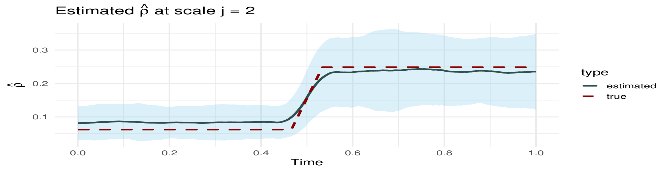
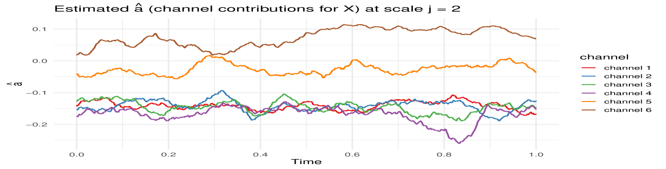
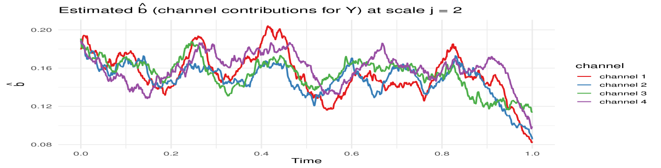
MvLSW-based simulation. We generate the multivariate time series from a MvLSW process with , observed across time points. The process is constructed using non-decimated Haar wavelets, with non-zero spectral structure specified at scale , as detailed in Appendix C.1. We impose a weaker dependence structure between and in the interval , and a stronger dependence in the interval , allowing us to examine the framework’s sensitivity to changes in cross-group coherence. Using the process realization (Figure 9) we estimate WaveCanCoh using Algorithm 1. To assess the estimation accuracy and account for variability, we replicate the simulation and estimation process 1000 times. At each time point, we compute the average of the estimated WaveCanCoh across the replicates and construct a 95% Wald confidence interval using the empirical variance. Figure 2 (left) demonstrates that the proposed WaveCanCoh method accurately tracks the true coherence structure and effectively reflects its time-varying nature, while the estimated canonical direction vectors in Figure 3 map the temporal and individual channel heterogeneity in their roles within the multivariate dependence structure.
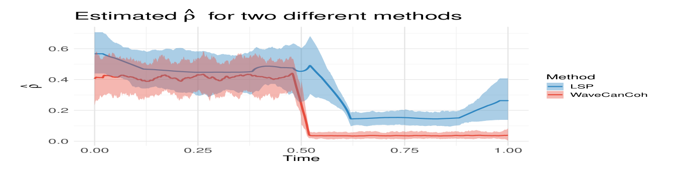
Mixture of AR(2)-based processes. To evaluate the robustness and generality of the proposed framework, we investigate WaveCanCoh using synthetic data generated from a mixture of AR(2) processes. Unlike the MvLSW-based simulations, this setting introduces nonstationary dynamics without any wavelet-based structure, providing a more flexible and realistic test scenario. To the best of our knowledge, WaveCanCoh is the first framework designed to estimate time-varying canonical coherence between two multivariate time series groups. However, to benchmark its performance, we compare it against a method based on the time-varying Cramér representation (Dahlhaus, 1997), with canonical coherence estimated via STFT-based localized spectra (Allen and Rabiner, 1977). We simulate 500 replicates of and , with , each formed by mixing five latent AR(2) sources tuned to neural frequency bands. In the first half, shared gamma () bands induce cross-group coherence, while the second half contains no shared structure (see details in Appendix C.2). Figure 2 (right) illustrates that while both methods detect the existence of coherence in the first half, only WaveCanCoh captures its sharp drop and true behaviour in the second half, thus demonstrating its advantage in identifying transient, localized changes that global Fourier-based methods fail to detect.
6 Local field potential (LFP) data analysis
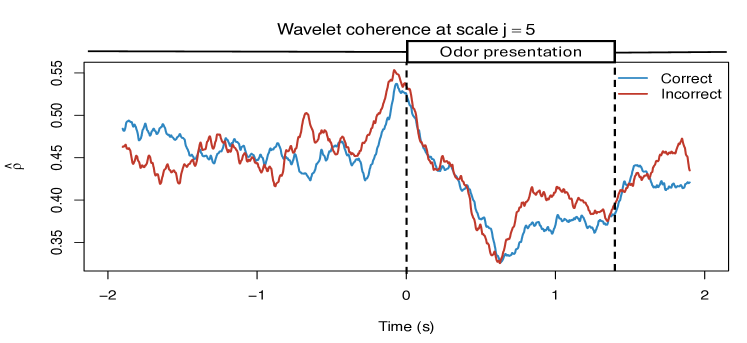
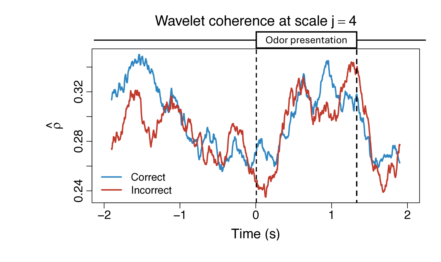
To demonstrate the practical utility of our proposed WaveCanCoh framework, we analyze LFP activity recorded from the hippocampus of rats engaged in a sequence memory task (Allen et al., 2016; Shahbaba et al., 2022). The data were recorded using a 22-electrode microdrive implanted in the CA1 subregion to capture high-resolution LFP signals across all channels at a sampling rate of . In this task, rats were tested on their memory of a sequence of five odors (odors ABCDE). Each odor was presented for 1.2 second () and a variable delay of 5 separated each odor (see Figure 1). For each trial (i.e., each odor presentation), the rat had to judge whether the odor was presented "in sequence" (e.g., ABC…) or "out of sequence" (e.g., ABD…) and indicate their decision by holding their nosepoke response until a tone signal (at 1.2) or withdrawing before the signal, respectively. Correct-response trials (i.e., correct "in sequence" or "out of sequence" decisions) were rewarded. LFP activity data were recorded over a 4 period ( time points) per trial, with marking the moment the rat initiated a nosepoke to receive the odor stimulus. This paradigm provides a well-controlled setting to investigate dynamic, time-varying functional interactions in the hippocampus during memory-guided decisions. We employ WaveCanCoh framework to quantify frequency-specific functional coherence between two groups of hippocampal electrodes (T1, T2, T4, T5 and T13–T17), and to examine how coherence patterns differ between correct- and incorrect-response trials ("in sequence" trials only). Specifically, we analyze LFP data from the rat Mitt, which included 40 correct-response trials and 32 incorrect-response trials. Figure 4 presents the estimated wavelet canonical coherence at scale , corresponding to the frequency band. The results, averaged across trials for each condition, reveal dynamic changes in inter-regional coherence, with a pronounced peak around the time of odor stimulus delivery (). Notably, distinct patterns emerge between correct and incorrect trials, suggesting that coherent activity in this frequency band may play a role in supporting successful memory retrieval and decision making. More results for several other scales can be found in Figure 10 in Appendix D.1.
To further interpret the coherence patterns, Figure 5 provides a spatial summary of the canonical coherence between the two electrode groups at several selected time points. The double-headed arrows represent the magnitude of estimated coherence between the two regions, while the numbers in the circles reflect the individual channel contributions to the global coherence, derived from the elements of the canonical vectors and .
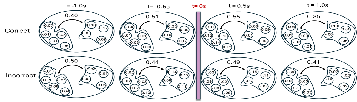
The results highlight that both the strength and structure of inter-regional coherence vary dynamically over time and differ across trial outcomes, reflecting the nonstationary nature of neural interactions during task performance. Specifically, incorrect-response trials exhibit lower coherence at time points immediately following the odor stimulus delivery and are often driven by a few dominant channels, while correct trials show higher coherence values and relatively balanced contributions across channels. These findings illustrate the necessity of a framework like WaveCanCoh, which simultaneously identifies time-varying and scale-specific dependence structures between multivariate time series. Traditional stationary or pairwise approaches would fail to capture such nuanced dynamics, highlighting the need for a method like WaveCanCoh to extract such complex relationships in brain activity. The directed interactions between brain regions are also explored in Appendix E with proposed Causal-WaveCanCoh framework.
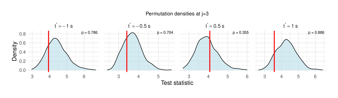
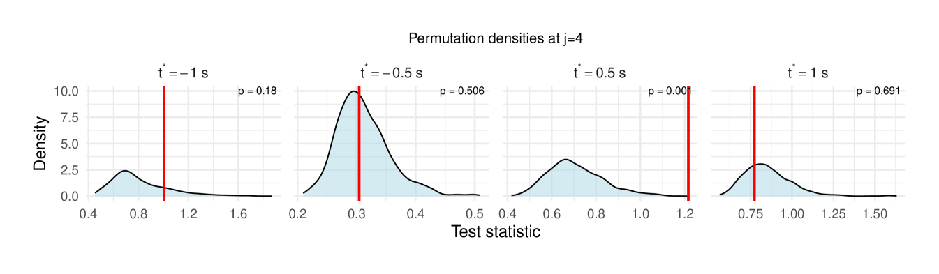
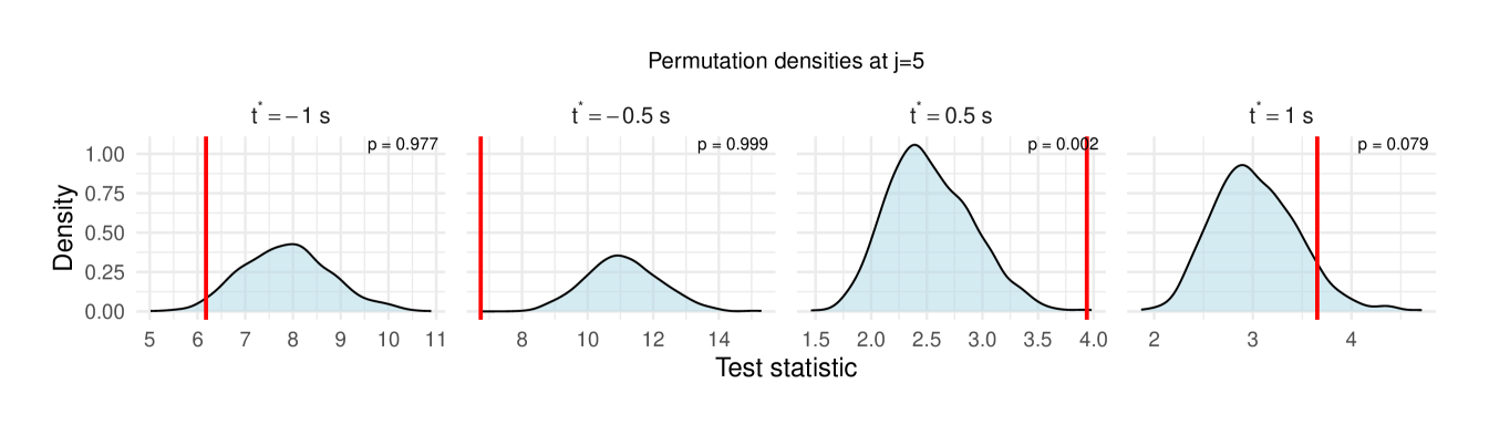
To further validate the existence of significant differences in the activity between correct- and incorrect-response trials, we propose a time-specific detection procedure based on the permutation test to determine temporally localized differences in the wavelet canonical coherence at a given scale between conditions, while maintaining the nonparametric nature of the statistical inference. The detailed inference procedure steps are shown in Algorithm 2 (Appendix D.2) and the results of the time-specific permutation test for WaveCanCoh across five wavelet scales and four selected time points are summarized in Table 1 (Appendix D.3). Statistically significant differences in canonical coherence between correct and incorrect trials emerge at time points following odor sampling (), predominantly at intermediate wavelet scales corresponding approximately to the frequency range. On the other hand, no significant differences between the two groups are observed prior to stimulus onset, indicating that the coherence patterns distinguishing inter-regional communication among trial types are tightly linked to task engagement. These findings demonstrate the effectiveness of the proposed WaveCanCoh framework and associated permutation test in capturing localized, frequency-specific differences in neural coordination between behavioral conditions, thus offering a powerful tool for analyzing complex brain interactions.
7 Conclusions
In this paper we introduced a novel methodological framework, scale-specific wavelet canonical coherence (WaveCanCoh), designed to quantify the dynamic multiscale coherence between two sets of nonstationary multivariate time series. Our primary contributions include the rigorous definition of WaveCanCoh within the multivariate locally stationary wavelet (MvLSW) framework and the development of a comprehensive estimation and theoretically-backed inference procedure based on wavelet analysis. We validated our proposed methodology through simulation studies, demonstrating its accuracy in tracking true coherence structures. The application to local field potential (LFP) activity recorded from subregions of the hippocampus effectively showcased the capability of WaveCanCoh to identify nuanced spatio-temporal coherence patterns associated with cognitive performance, while our permutation-based inference procedure provided a robust, nonparametric approach for detecting significant coherence differences between conditions. Compared to existing stationary and Fourier-based canonical coherence methods, WaveCanCoh is shown to offer significant advantages, particularly through its ability to adaptively capture transient and time-localized interactions, hence it is highly suitable for analyzing signals in neuroscience and other fields with data exhibiting dynamic cross-group interactions.
References
- Allen and Rabiner (1977) J.B. Allen and L.R. Rabiner. A unified approach to short-time fourier analysis and synthesis. Proceedings of the IEEE, 65(11):1558–1564, 1977.
- Allen et al. (2016) Timothy A. Allen, Daniel M. Salz, Sam McKenzie, and Norbert J. Fortin. Nonspatial sequence coding in ca1 neurons. The Journal of Neuroscience, 36(5):1547–1563, 2016.
- Box and Tiao (1977) G. E. P. Box and G. C. Tiao. A canonical analysis of multiple time series. Biometrika, 64(2):355–365, August 1977.
- Brillinger (2001) D. R. Brillinger. Time Series: Data Analysis and Theory. SIAM, 2001.
- Dahlhaus (1997) Rainer Dahlhaus. Fitting time series models to nonstationary processes. The Annals of Statistics, 25(1):1–37, February 1997.
- Daubechies (1992) Ingrid Daubechies. Ten lectures on wavelets. SIAM, 1992.
- Embleton et al. (2022) Jonathan Embleton, Marina I. Knight, and Hernando Ombao. Multiscale spectral modelling for nonstationary time series within an ordered multiple-trial experiment. Annals of Applied Statistics, 16(4):2774–2803, 2022.
- Geweke (1982) John Geweke. Measurement of linear dependence and feedback between multiple time series. Journal of the American Statistical Association, 77(378):304–313, June 1982.
- Grinsted et al. (2004) A. Grinsted, J. C. Moore, and S. Jevrejeva. Application of the cross wavelet transform and wavelet coherence to geophysical time series. Nonlinear Processes in Geophysics, 11(5-6):561–566, 2004.
- Hotelling (1936) Harold Hotelling. Relations between two sets of variates. Biometrika, 28(3/4):321–377, 1936.
- Huang et al. (2004) Hsiao-Yun Huang, Hernando Ombao, and David S. Stoffer. Discrimination and classification of nonstationary time series using the slex model. Journal of the American Statistical Association, 99(467):763–774, 2004.
- Knight et al. (2024) Marina I. Knight, Matthew A. Nunes, and Jessica K. Hargreaves. Adaptive wavelet domain principal component analysis for nonstationary time series. Journal of Computational and Graphical Statistics, 33(3):941–954, 2024.
- Mardia et al. (1979) K. V. Mardia, J. T. Kent, and J. M. Bibby. Multivariate Analysis. Academic Press, 1979.
- Nason (2008) G. P. Nason. Wavelet Methods in Statistics with R. Springer New York, NY, 2008.
- Nason et al. (2000) Guy P. Nason, Rainer Sachs, and Gerald Kroisandt. Wavelet processes and adaptive estimation of the evolutionary wavelet spectrum. Journal of the Royal Statistical Society: Series B (Statistical Methodology), 62(2):271–292, 2000.
- Ombao and Pinto (2024) Hernando Ombao and Marco Pinto. Spectral dependence. Econometrics and Statistics, 32:122–159, 2024.
- Park et al. (2014) Timothy Park, Idris Eckley, and Hernando Ombao. Estimating time-evolving partial coherence between signals via multivariate locally stationary wavelet processes. IEEE Transactions on Signal Processing, 62:5240–5250, 2014.
- Shahbaba et al. (2022) Babak Shahbaba, Lu Li, Francesco Agostinelli, Meenakshi Saraf, Keiland W. Cooper, Daniel Haghverdian, George A. Elias, Pierre Baldi, and Norbert J. Fortin. Hippocampal ensembles represent sequential relationships among an extended sequence of nonspatial events. Nature Communications, 13(1):787, February 2022.
- Talento et al. (2024) Mara Sherlin D. Talento, Sarbojit Roy, and Hernando C. Ombao. Kencoh: A ranked-based canonical coherence. arXiv preprint arXiv:2412.10521, December 2024.
- Viduarre et al. (2019) C. Viduarre, G. Nolte, I.E.J. de Vries, M. Gómez, T.W. Boonstra, K.-R. Müller, A. Villringer, and V.V. Nikulin. Canonical maximization of coherence: A novel tool for investigation of neuronal interactions between two datasets. NeuroImage, 201:116009, November 2019.
- West et al. (1999) Mike West, Raquel Prado, and Andrew D. Krystal. Evaluation and comparison of eeg traces: Latent structure in non-stationary time series. Journal of the American Statistical Association, 94(446):1083–1095, 1999.
Appendix
Appendix A Basic introduction to wavelets
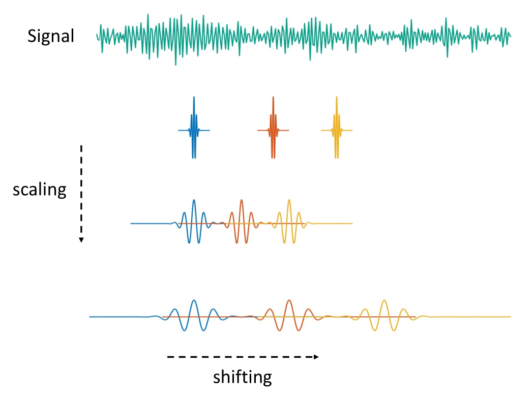
Wavelet analysis provides a powerful framework for studying signals with both time- and scale-varying structure, making it particularly well-suited for nonstationary data. Unlike traditional Fourier-based methods, which decompose signals into global sinusoidal bases and therefore assume stationarity, wavelets enable localized, adaptive decompositions by projecting signals onto functions that are compact in both time and scale. This localization is achieved through two core operations: scaling, which adjusts the width of the wavelet to analyze different resolution levels, and shifting, which moves the wavelet across time to detect when features occur. Specifically, the wavelet functions at scale and shift , denoted by , are derived from a mother wavelet and defined as
where represents the number of scales. Smaller scale corresponds to finer (high-frequency) resolution, and larger captures coarser (low-frequency) trends. A similar construction applies to the father wavelet, denoted by , which serves as a scaling function (see Daubechies (1992) and Nason (2008) for more details on wavelets). Figure 6 illustrates the effect of scaling and shifting operations on the wavelet function. This ability to isolate both short-lived and long-term features distinguishes wavelet methods from Fourier analysis, allowing for nuanced investigation of nonstationary signals such as neural activity, where structure evolves dynamically across time and scale.
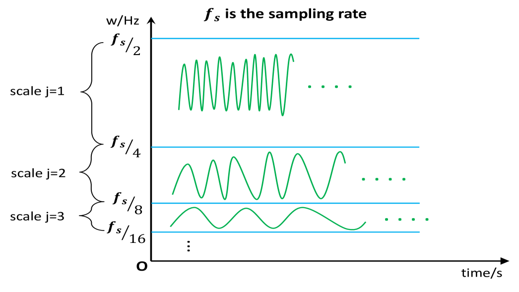
The correspondence between wavelet scale and signal frequency arises from the principle of multi-resolution analysis, which provides the foundational framework for wavelet construction and signal representation. Briefly, the discrete wavelet transform (DWT) decomposes a signal into frequency subbands via a dyadic filter bank architecture. At each level, the signal is passed through a pair of conjugate quadrature filters: a low-pass filter and a high-pass filter , followed by downsampling by a factor of two. The low-pass branch yields approximation coefficients that retain coarse-scale information, while the high-pass branch produces detail coefficients that capture localized high-frequency variations. Specifically, given a discrete signal , the approximation and detail coefficients at level are obtained by
where is the approximation from the previous level (with ). This process is iterated on the low-pass output, producing a multiscale representation in which each level isolates a specific frequency band. For a signal sampled at rate , the detail coefficients at level correspond approximately to the frequency interval . The orthogonality between subbands ensures perfect reconstruction and energy preservation, and the hierarchical filter bank provides a localized time-frequency analysis with increasingly coarse temporal resolution at lower frequencies. The explanation above offers an intuitive understanding of how components at each wavelet scale can be approximated to true frequency bands (see Figure 7 for an intuitive illustration). This approximation enables our framework to capture the overall association between two sets of locally stationary time series in both the temporal and frequency domains (more details can be found in Daubechies (1992)).
Appendix B Theoretical proofs
Proof of solution to equation (10). Suppose that and are two multivariate time series and for each time point , the goal is to find the vectors and that maximize the coherence,
subject to the normalization constraints described in the main paper
Assuming rescaled time and scale are fixed, we suppress them for clarity. To solve the above optimization problem, we set up the Lagrangian as
Differentiating the Lagrangian with respect to and , respectively and requiring the partial derivatives to equal zero, we obtain
With , and since is a real-valued quantity, we further obtain
Recalling the constraints and , it immediately follows that
By substituting the above back into , and assuming to be non-zero, we obtain
which plugged into , , respectively, yield
Hence is an eigenvalue for both matrices
whose corresponding eigenvectors are and , respectively. Thus, the defined canonical coherence
is the largest eigenvalue of above matrices. The case when illustrates the canonical coherence between and is 0, which is not a meaningful scenario for this problem. We recall the above equations hold for every time and scale .
Proof of consistency of WaveCanCoh estimator. We aim to establish the consistency of the matrix estimators
According to Nason et al. (2000) and Park et al. (2014), the smoothed periodogram-based estimators of the local wavelet spectral (LWS) matrices are consistent. Specifically, as the number of time points and the smoothing parameter with , we have
Assuming the spectral matrices and their estimators are non-singular, it follows by the continuous mapping theorem that
Since matrix multiplication is continuous with respect to convergence in probability, we obtain the consistency of the matrix estimators by Slutsky’s theorem, namely
Consequently, the estimated wavelet canonical coherence and associated canonical vectors, derived from the largest eigenvalue and corresponding eigenvectors of and , also converge in probability to their population counterparts, following arguments akin to those in Knight et al. (2024).
Appendix C Details of the simulation setup
This appendix provides the full specification of the simulation experiments described in Section 5 of the main text.
C.1 MvLSW-based simulation
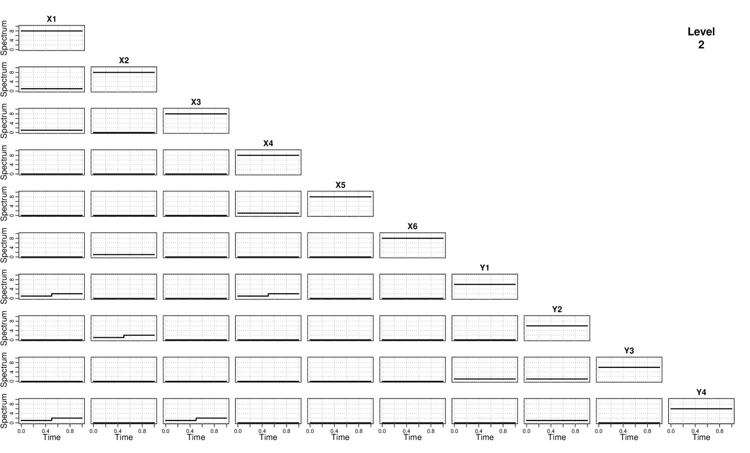
We simulate a dimensional multivariate time series from a multivariate locally stationary wavelet (MvLSW) process over time points. The wavelet spectrum is non-zero only at scale and is structured as a block matrix
Auto-spectral block:
Auto-spectral block:
Cross-spectral block:
This block is time-varying. For , each specified cross-group pair has coherence value 1; for , the same entries increase to 2.
Let
then
The entries of the cross-spectral matrix determine how individual channels contribute to the global coherence structure between and . Figure 8 visualizes the spectral structure , and Figure 9 shows example realizations of the simulated processes and .
C.2 Mixture of AR(2)-based simulation
Fourier-based LSP method for comparison
As a benchmark, we implement a method based on the time-varying Cramér representation for locally stationary processes (LSP), introduced in Dahlhaus (1997). A locally stationary process can be expressed as
where is a smoothly varying transfer function and is a complex orthogonal increment process with . The local spectral density is then defined as . We estimate via the Short-Time Fourier Transform (STFT) with a Gaussian smoothing kernel and compute canonical coherence over .
Simulation setting
We simulate 500 independent replicates of two multivariate processes, and , for , with and sampling rate . Each process is generated from mixture of latent AR(2) sources, , peaking at different frequency bands (delta, theta, alpha, beta, gamma), respectively. For the first half of the time series (), the observed processes are given by:
and for the second half ():
where the mixing matrices are:
For each row of the mixing matrices, a selected subset of frequency bands is assigned non-zero weights that are randomly drawn to sum to a predefined total (e.g., 0.95, 0.90, or 1.0), introducing controlled variability across replicates while preserving the intended contribution structure. The latent sources and are partially shared in the gamma band (component 5) during the first regime, with mixing weights and , respectively:
where is a common latent process. Specifically, each channel, say , of , and is generated from the following AR(2) process independently,
where is white noise and the coefficients are , . For each component , we use the frequency vector, , and the sharpness parameter , where smaller yields narrower frequency bands.
This design induces time-varying coherence between the first two channels of and during the first regime, primarily through the shared gamma component, while maintaining independence during the second regime. The abrupt transition in mixing structure at provides a controlled setting for evaluating the sensitivity of coherence estimation methods to sudden changes in cross-dependence.
Appendix D Additional analysis for the LFP data in Section 6
D.1 Additional results
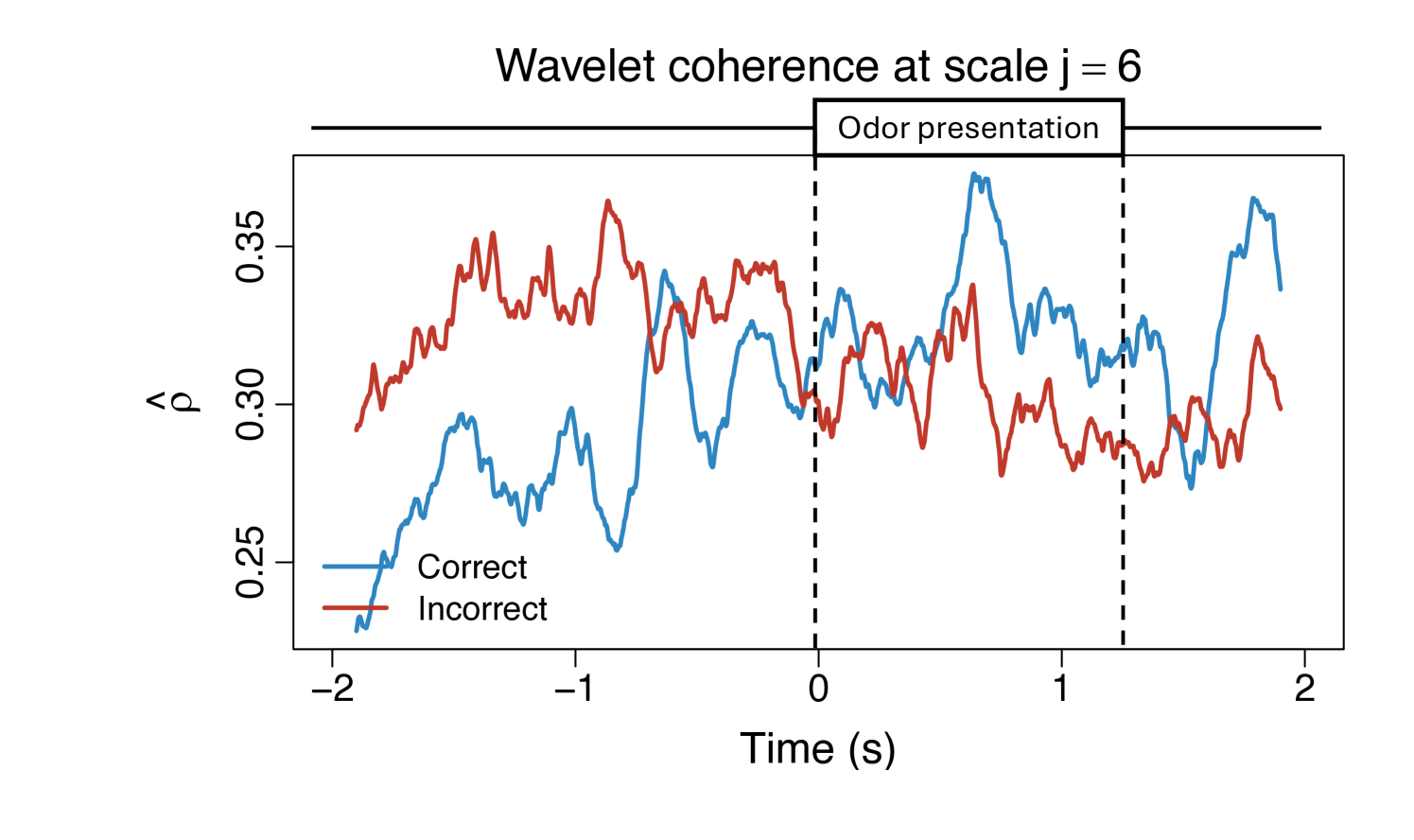
We display the estimated wavelet canonical coherence between two electrode clusters across additional scales. Figure 10 shows that cross-group associations vary significantly over time, with the stimulus clearly eliciting a scale-dependent response, indicative of the heterogeneous brain activity across different frequency bands. These results emphasize the importance of capturing scale-specific, time-varying coherence.
D.2 Permutation test: Algorithm
Algorithm 2 below gives the detailed procedure used in Section 6 for detecting significant differences in canonical coherence between correct- and incorrect-response trials, at selected time points.
-
•
Combine all values from both correct- and incorrect-response trials across the time window.
-
•
Perform random permutations. For each permutation :
-
–
Randomly assign trials into two new groups of the same sizes as the original groups.
-
–
Compute the permuted statistic:
where and are the permuted trial groups.
-
–
D.3 Permutation test: LFP results
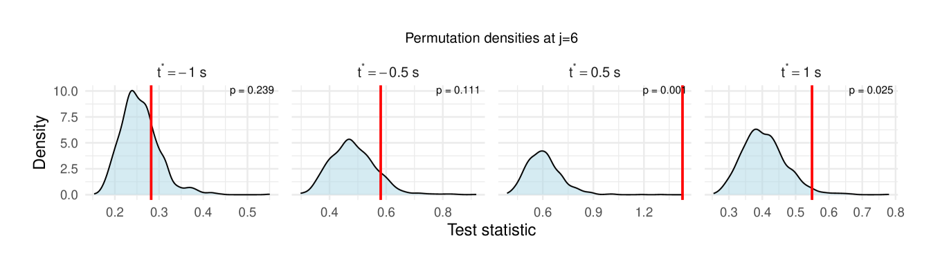
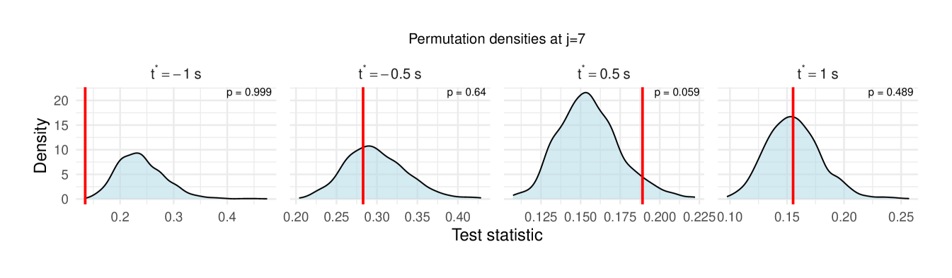
Table 1 reports the permutation test results on the LFP data, with the value in each cell representing the difference in the median wavelet coherence between correct and incorrect trials at the corresponding scale and time . The values in parentheses denote the permutation -values obtained using the windowed test procedure (window size ), with the number of permutation , and the detailed test results are shown in Figure 11, revealing significant differences between correct- and incorrect-response trials at scales to following the odor stimulation.
While our permutation-based inference procedure provides a robust, nonparametric approach for detecting significant coherence differences between conditions, nevertheless this framework does exhibit certain limitations, e.g., it inherently focuses on predefined wavelet scales rather than on arbitrary frequency bands, potentially restricting analyses that require precise frequency localization.
| -1.0 | -0.5 | 0.5 | 1.0 | |
| 3 () | 0.222 (0.786) | 0.068 (0.704) | -0.178 (0.355) | 0.106 (0.886) |
| 4 () | -0.090 (0.180) | -0.021 (0.506) | 0.023 (0.001**) | 0.027 (0.691) |
| 5 () | 0.006 (0.977) | 0.229 (0.999) | 0.334 (0.002**) | 0.016 (0.079) |
| 6 () | -0.025 (0.239) | -0.049(0.111) | 0.039 (0.001**) | 0.002 (0.025**) |
| 7 () | -0.014 (0.999) | 0.058 (0.640) | 0.012 (0.059) | -0.030 (0.489) |
Appendix E Causal-WaveCanCoh analysis
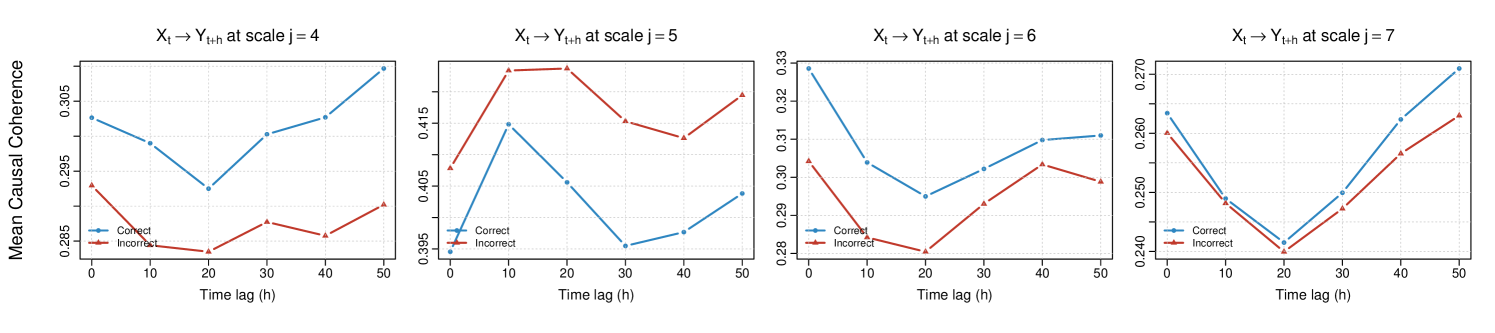
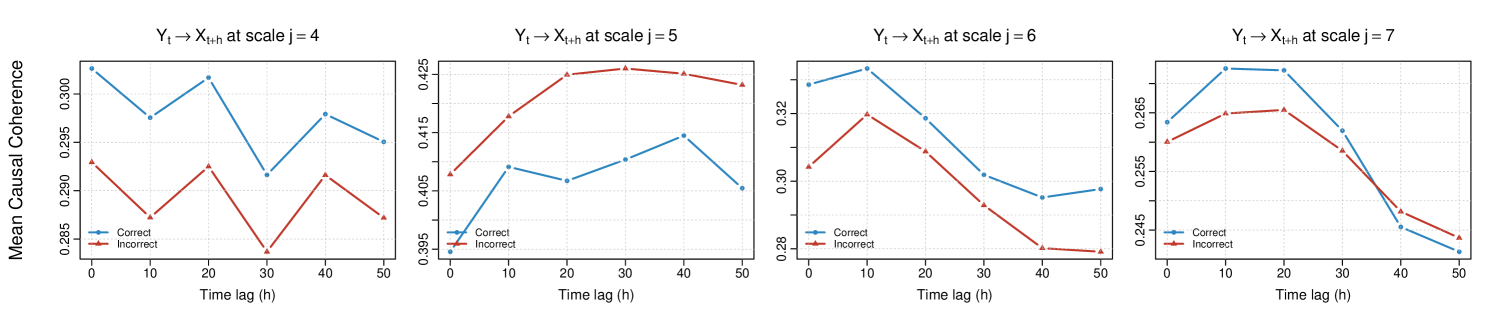
To further explore directed interactions between brain regions, we implement the Causal-WaveCanCoh framework (equation (17)) on LFP activity data, which extends WaveCanCoh by introducing a lead-lag structure to evaluate time-lagged canonical coherence. Specifically, we define and as the multivariate signals corresponding to the two investigated distinct hippocampal regions, and we conduct the analysis in both directions, namely and , for lags , corresponding to time shifts from 0 (contemporaneous dependence, used as reference point) to 0.05 seconds.
Figure 12 shows the average scale-specific estimated causal canonical coherence for both directions across the odor presentation time () and trial type (correct- vs incorrect-response trials). The results reveal lag-dependent and scale-driven patterns of directed coherence that identify a stronger association between the two hippocampal regions at scale (corresponding to the frequency band ). This notably occurs in both directions, with the activity in T13-T17 leading that of T1-T5 in correct-response trials after . The strength and behavior of coherence vary across scales, as well as across correct- and incorrect-response trial groups, which can be captured by our Causal-WaveCanCoh framework.