Weak solutions to the stationary Cahn-Hillard/Navier-Stokes equations for compressible fluids
Abstract.
We are concerned with the Cahn-Hilliard/Navier-Stokes equations for the stationary compressible flows in a three-dimensional bounded domain. The governing equations consist of the stationary Navier-Stokes equations describing the compressible fluid flows and the stationary Cahn-Hilliard type diffuse equation for the mass concentration difference. We prove the existence of weak solutions when the adiabatic exponent satisfies . The proof is based on the weighted total energy estimates and the new techniques developed to overcome the difficulties from the capillary stress.
Key words and phrases:
Stationary equations, weak solutions, Navier-Stokes, Cahn-Hilliard, mixture of fluids, diffuse interface.2010 Mathematics Subject Classification:
35Q35, 76N10, 35Q30, 34K21, 76T10.1. Introduction
The Cahn-Hilliard/Navier-Stokes system is one of the important diffuse interface models (cf.[3, 8, 17]) describing the evolution of mixing fluids. The mixture is assumed to be macroscopically immiscible, with a partial mixing in a small interfacial region where the sharp interface is regularized by the Cahn-Hilliard type diffusion in terms of the mass concentration difference. Roughly speaking, the Cahn-Hilliard equation is used for modeling the loss of mixture homogeneity and the formation of pure phase regions, while the Navier-Stokes equations describe the hydrodynamics of the mixture that is influenced by the order parameter, due to the surface tension and its variations, through an extra capillarity force term.
In this paper, we are interested in the following stationary Cahn-Hilliard/Navier-Stokes system for the mixture of compressible fluid flows in a three-dimensional bounded domain :
| (1.1) |
where denotes the total density, the mean velocity field, the mass concentration difference of the two components, the chemical potential, and the external force; the tensor
| (1.2) |
is the Navier-Stokes stress tensor, where is the identity matrix, are constant such that
| (1.3) |
the tensor
| (1.4) |
is the capillary stress tensor; and
| (1.5) |
is the pressure with the free energy density (cf. [1, 17])
| (1.6) |
where is the adiabatic exponent, and are two given functions. The corresponding evolutionary diffuse interface model was derived in [1, Section 2.2] where the existence of weak solutions was obtained for . We refer the readers to [3, 8, 17, 1, 16] for more discussions on the physics and models of mixing fluids with diffuse interfaces.
We briefly review some related results in literature. For the stationary Navier-Stokes equations of compressible flows, the existence of weak solutions was studied in Lions [15] with , Novotný-Strašcraba [20] with , Frehse-Steinhauer-Weigant [12] with , Plotnikov-Weigant[24] with , as well as in Jiang-Zhou [14] and Bresch-Burtea [7] for periodic domains. For the stationary Cahn-Hilliard/Navier-Stokes equations of incompressible flows, the existence of weak solutions was obtained in Biswas-Dharmatti-Mahendranath-Mohan [5], Ko-Pustejovska-Suli [22], and Ko-Suli [23]. For the compressible Cahn-Hilliard/Navier-Stokes equations, Liang-Wang in [16] proved the existence of weak solutions in case of the adiabatic exponent See [15, 20, 10, 12, 24, 14, 19, 18, 5, 22, 23, 16, 7, 6, 9] and their references for more results.
In this paper, we shall continue our study on the existence of weak solutions, and improve our previous result obtained in [16] for to the case of for the stationary equations (1.1) subject to the following boundary conditions:
| (1.7) |
and the additional conditions:
| (1.8) |
with two given constants and , where is the normal vector of .
Before stating our main results, we introduce some notation that will be used throughout this paper. For two given matrices and , we denote their scalar product by . For two vectors , denote We use for simplicity. For any and integer is the standard Sobolev space (cf. [2]), and
where is the average of over .
As in [16], we define the weak solution as follows.
Definition 1.1.
The vector of functions is called a weak solution to the problem (1.1)-(1.8), if
for some and , and the following properties hold true:
(i) The system is satisfied in the sense of distributions in , and (1.8) holds for the given constants and
(ii) If is prolonged by zero outside , then both the equation and
are satisfied in the sense of distributions in , where with if is large enough.
(iii) The following energy inequality is valid:
We now state our main result.
Theorem 1.1.
The main contribution of this paper is to develop new ideas to improve the existence result of [16] from the adiabatic exponent in [16] to a wider range . Our approach is mainly motivated by the papers [14, 24] where the authors studied the existence of weak solutions to the stationary Navier-Stokes equations of compressible fluids. In order to prove the Theorem 1.1, we start with the approximate solution sequence stated in Proposition 2.1 in Section 2, and use the weighted total energy as in [14, 24] together with new techniques to handle the capillary stress to establish the uniform in bound on in (3.1). Then, we shall be able to take the limit as and complete the proof of Theorem 1.1 by means of the weak convergence arguments in [16]. More precisely, our proof includes the following key ingredients and new ideas:
- (1)
-
(2)
In order to analyze the weighted total energy we need to overcome the new difficulties caused by the capillary stress in (1.4), besides the Navier-Stokes stress tensor . In particular, we are required to control appearing in (3.10) and (3.11). For this purpose we make the following estimate
where is small and . By virtue of the Finite Coverage Theorem, can be covered by a finite number of balls of radius centered at , then
Next, we assume the following a priori bound
(1.11) that is uniform in If we select small enough such that
we are able to derive the following estimate
-
(3)
With the above two key steps, we can show that there is a constant that does not rely on M, such that
as long as . This yields , and then we have the estimate for some positive constant independent of M. By choosing the a priori bound , one can close the a priori assumption (1.11) and prove the existence of weak solutions in the Theorem 1.1.
The rest of the paper is organized as follows. In Section 2, we present the approximate solutions constructed in [16] and provide some preliminary lemmas. In Section 3, we prove the Theorem 1.1.
2. Approximate Solutions and Preliminaries
We start with the following approximate solutions constructed in [16].
Proposition 2.1 (Theorem 4.1, [16]).
Lemma 2.1.
Proof.
The next lemma gives an embedding from to in a three-dimensional bounded domain, via the Green representation formula.
Lemma 2.2.
Let be a bounded domain with boundary and satisfy
for some constant . Then, there is a constant which depends only on , such that
(i) If then
| (2.8) |
(ii) If and , then
| (2.9) |
Proof.
The proof of the case (i) can be found in [24, Lemma 4]. Here we prove the case (ii). Let be a solution to the Neumann boundary value problem:
| (2.10) |
Recalling the Green representation formula , we have
| (2.11) |
Thanks to (2.10), using integration by parts yields
| (2.12) |
From (2.12) we then derive the following estimate:
which implies
Substituting the above inequality into (2.12) gives that
Then (2.9) follows from (2.11). The proof of Lemma 2.2 is completed. ∎
Lemma 2.3 (Bogovskii).
Let be a bounded Lipschitz domain. There is a linear operator for , such that, for ,
(i)
(ii)
3. Proof of Theorem 1.1
For the approximate solution given in Proposition 2.1, if we can show that there is a constant uniform in such that
| (3.1) |
then, from (3.1) we are able to control the possible oscillation of density and the nonlinearity in the free energy density (1.6), and hence we can take the limit as to prove that the approximate solution converges weakly to some limit function which satisfies (1.1)-(1.8) in the sense of Definition 1.1. This convergence proof relies heavily on the compactness arguments in [10, 16, 15, 21] and the details can be found in [16]. Therefore, it suffices to prove the following proposition in order to complete the proof of Theorem 1.1.
Proposition 3.1.
Remark 3.1.
For the sake of simplicity of notation, in the proof of the Proposition 3.1 below we will drop the subscript in and denote it by .
Lemma 3.1.
Proof.
Remark 3.2.
Next, we shall deduce some weighted estimates on the pressure and kinetic energy together, i.e., the weighted total energy motivated by [14, 24]. As in [12], we introduce
| (3.8) |
where the function can be regarded as the distance function when is close to the boundary, smoothly extended to the whole domain In particular,
| (3.9) |
where the constants , , are given. See for example [26, Exercise 1.15] for details.
Lemma 3.2.
Let be the solutions stated in Proposition 2.1. Then, for , the following properties hold:
(ii) In case of we have
| (3.11) | ||||
where and is independent of or .
Proof.
In order to prove Lemma 3.2 we borrow some ideas developed in [12, 19, 24] and modify the proof in [16].
Stpe 1: Proof of (3.10): From (3.8) and (3.9) we see that with . Furthermore, by (3.9) and the fact , one has
| (3.14) |
With (3.9) and (3.14), one deduces that, for
| (3.15) | ||||
Thanks to (3.12), we multiply by to obtain
| (3.16) | ||||
By (1.10), (2.2)-(2.3), (3.15), and the fact , we estimate the right-hand side of (3.16) as
| (3.17) | ||||
and
| (3.18) |
For the left-hand side of (3.16), it holds from (3.13) and (3.15) that
| (3.19) | ||||
By (3.9), one has
Then,
Thus we have the following computation and estimate:
| (3.20) | ||||
where we have used (3.14) and the Cauchy inequality. Therefore, taking (3.17)-(3.20) into account, using (3.7), (3.3), and , we deduce from (3.16) that
| (3.21) | ||||
Finally, thanks to (2.3) and (3.13), one has
| (3.22) | ||||
Stpe 2: Proof of (3.11): Let , and be the smooth cut-off function satisfying
| (3.23) |
If we multiply by , we get
| (3.24) | ||||
From the following computation,
one sees that the second term on the left-hand side of (3.24) satisfies
| (3.25) | ||||
where the constant is independent of and for the last inequality we have used for any Owing to (3.23), (3.7), and the fact
we have the following estimates:
| (3.26) | ||||
and
| (3.27) | ||||
where is independent of
With the above three estimates (LABEL:325)-(LABEL:327) in hand, we deduce from (3.24) that
| (3.28) | ||||
By (3.21)-(3.22) and the following estimate
we obtain from (LABEL:328) that
| (3.29) | ||||
It remains to deal with the last term in (3.29). To this end, we use the ideas developed in [16] and divide the proof into two cases: is far away from the boundary; is close to the boundary.
For the case of with being taken from (3.9), it is clear that
| (3.30) |
With (3.30), as well as (3.12)-(3.13), (3.22), Lemma 3.1, we deduce from (3.29) that
| (3.31) | ||||
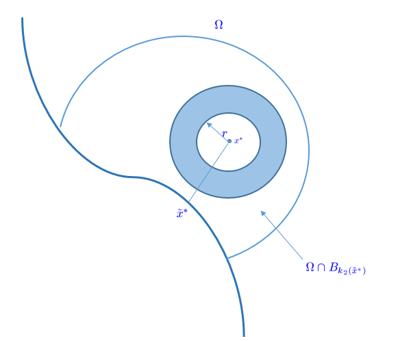
For the case of close to the boundary, that is, , let with Then, one deduces (see Figure 1 below) that
| (3.32) |
The next lemma provides a refined estimate on the weighted energy obtained in Lemma 3.2.
Lemma 3.3.
Let the assumptions in Lemma 3.2 hold true. Assume that there is a constant uniform in , such that
| (3.35) |
Then,
| (3.36) |
Proof.
If it holds that, for any ,
| (3.37) | ||||
Combining (3.37) with (3.10), we obtain for any ,
| (3.38) | ||||
where the constant is independent of or . Using (2.2), (2.5), and the interpolation inequality, we have the following estimate:
| (3.39) | ||||
where, and in what follows, the constant is independent of M. Choosing small so that
| (3.40) |
It follows from (3.38) that
| (3.41) | ||||
where, for the last two inequalities, we have used (3.39) and (3.40).
The final two Lemmas 3.4 and 3.5 are devoted to proving the desired inequality (3.1) and the a priori bound (3.35).
Lemma 3.4.
Let the assumptions in Proposition 3.1 hold true. Then
| (3.43) |
Proof.
Define
| (3.44) |
By (3.2), one has
| (3.45) |
Thanks to (2.2) and the Hölder inequality, it holds that
| (3.46) |
and
| (3.47) |
By means of (1.3), (1.10), (2.4), (3.46), we get
| (3.48) |
Let
| (3.49) |
One calculates as the following,
| (3.50) |
where since Hence, utilizing (3.36), (3.47), (3.48), we integrate (3.50) and obtain
| (3.51) | ||||
From (3.48), (3.51), and Part (i) in Lemma 2.2, one deduces
which together with (3.45) yields
| (3.52) |
Combining (3.52) with (3.48), we get (3.43). The proof of Lemma 3.4 is completed. ∎
Lemma 3.5.
Let the assumptions in Theorem 3.1 hold true. Then,
| (3.53) |
Proof.
Owing to (3.44) and (3.49), one has
By (3.2), (3.51), (3.52), and the Hölder inequality, we have the following estimate,
| (3.54) | ||||
Hence, using (3.48), (3.52), (3.54), Part (ii) in Lemma 2.2, we find
| (3.55) |
On the other hand, it follows from (2.2), (3.54), Lemma 2.1, Lemma 3.4, and the interpolation inequality that
| (3.56) |
Therefore, utilizing (3.55)-(3.56) and the fact , we conclude
| (3.57) | ||||
Substituting (3.57) into (3.3), using (3.47), (3.48), (3.52), we get
| (3.58) | ||||
Thanks to (3.2), one has
| (3.59) |
The combination of (3.58) with (3.59) gives rise to
| (3.60) |
where depends only on . From (3.60), there is a constant independent of , such that
and hence we are allowed to select in (3.35)
| (3.61) |
and close the a priori assumption in (3.35).
It only remains to derive the bound of From (1.6), (3.57), (3.60), it follows that
| (3.62) | ||||
From (2.3) and (3.60), the same argument as (2.7) yields
which implies
| (3.63) |
Then (3.63) and (3.62) provide us the following estimate:
| (3.64) |
In conclusion, the desired estimate (3.53) follows from (2.5), (3.48), (3.52), (3.60), and (3.64). The proof of Lemma 3.5 is completed. ∎
Acknowledgement
The research of D. Wang was partially supported by the National Science Foundation under grant DMS-1907519. The authors would like to thank the anonymous referees for valuable comments and suggestions.
References
- [1] H. Abels, E. Feireisl, On a diffuse interface model for a two-phase flow of compressible viscous fluids, Indiana Univ. Math. J. 57(2) (2008), 659-698.
- [2] R. Adams, Sobolev spaces, New York: Academic Press, 1975.
- [3] D. Anderson, G. McFadden, A. Wheeler, Diffuse-interface methods in fluid mechanics, Annu. Rev. Fluid Mech., 30, Annual Reviews, Palo Alto, CA, (1998) 139-165.
- [4] L. Antanovskii, A phase field model of capillarity, Phys. Fluids A 7 (1995), 747-753.
- [5] T. Biswas, S. Dharmatti, P. Mahendranath, M. Mohan, On the stationary nonlocal Cahn-Chilliard-Navier-Stokes system: existence, uniqueness and exponential stability. Asymptotic Analysis 125 (2021), no. 1-2, 59-99.
- [6] T. Biswas, S. Dharmatti, M. Mohan, Second order optimality conditions for optimal control problems governed by 2D nonlocal Cahn-Hillard-Navier-Stokes equations. Nonlinear Stud 28 (2021), no. 1, 29-43.
- [7] D. Bresch, C. Burtea, Weak solutions for the stationary anisotropic and nonlocal compressible Navier-Stokes system. J. Math. Pures Appl. (9) 146 (2021), 183-217.
- [8] J. Cahn, J. Hilliard, Free energy of non-uniform system. I. Interfacial free energy, J. Chem. Phys. 28 (1958), 258-267.
- [9] S. Chen, S. Ji, H. Wen, C. Zhu, Existence of weak solutions to steady Navier-Stokes/Allen-Cahn system. J. Differential Equations 269 (2020), no. 10, 8331-8349.
- [10] E. Feireisl, Dynamics of viscous compressible fluids, Oxford University Press (2004).
- [11] Galdi, An Introduction to the Mathematical Theory of the Navier-Stokes Equations, I. Spinger- Verlag, Heidelberg, New-York, 1994.
- [12] J. Frehse, M. Steinhauer, W. Weigant, The Dirichlet problem for steady viscous compressible flow in three dimensions, J. Math. Pures Appl. 97 (2012), 85-97.
- [13] D. Gilbarg, N. Trudinger, Elliptic Partial Differential Equations of Second Order, 2nd edition, Grundlehren Math. Wiss., vol. 224, Springer-Verlag, Berlin, Heidelberg, New York, 1983.
- [14] S. Jiang, C. Zhou, Existence of weak solutions to the three-dimensional steady compressible Naiver-Stokes equations, Ann. Inst. H. Poincaré Anal. Non Linéaire 28 (2011) 485-498.
- [15] P. Lions, Mathematical topics in fluid mechanics. Vol. 2. Compressible models. Oxford Lecture Series in Mathematics and its Applications, 10. Oxford Science Publications. The Clarendon Press, Oxford University Press, New York, 1998.
- [16] Z. Liang, D. Wang, Stationary Cahn-Hilliard-Navier-Stokes equations for the diffuse interface model of compressible flows, Math. Mod. Meth. Appl. Sci. 30 (2020), 2445-2486.
- [17] J. Lowengrub, L. Truskinovsky, Quasi-incompressible Cahn-Hilliard fluids and topological transitions, Proc. R. Soc. Lond. A 454 (1998), 2617-2654.
- [18] P. B. Mucha, M. Pokorný, On a new approach to the issue of existence and regularity for the steady compressible Navier-Stokes equations, Nonlinearity 19, (2006), 1747-1768.
- [19] P. B. Mucha, M. Pokorný, E. Zatorska, Existence of stationary weak solutions for compressible heat conducting flows. Handbook of Mathematical Analysis in Mechanics of Viscous Fluids, 2595-2662, Springer, Cham, 2018.
- [20] S. Novo, A. Novotný, On the existence of weak solutions to the steady compressible Navier-Stokes equations when the density is not square integrable, J. Math. Fluid Mech. 42 3 (2002), 531-550.
- [21] A. Novotný, I. Stras̆kraba, Introduction to the Mathematical Theory of Compressible Flow. Oxford Lecture Series in Mathematics and its Applications, 27. Oxford University Press, Oxford, 2004.
- [22] S. Ko, P. Pustejovska, E. Suli, Finite element approximation of an incompressible chemically reacting non-Newtonian fluid, Math. Mod. Numerical Appl. 52(2) (2018), 509-541.
- [23] S. Ko, E. Suli, Finite element approximation of steady flows of generalized Newtonian fluids with concentration-dependent power-law index, Math. Comp. 88 (2019), no. 317, 1061-1090.
- [24] P. I. Plotnikov, W. Weigant, Steady 3D viscous compressible flows with adiabatic exponent , J. Math. Pures Appl. 104 (2015) 58-82.
- [25] E. Stein, Singular integrals and differentiability properties of functions, Princeton Univ. Press, Princeton, New Jersey, 1970.
- [26] W. P. Ziemer, Weakly Differentiable Functions. Springer, New York, 1989.