Weak Supervision with Incremental Source Accuracy Estimation
Abstract
Motivated by the desire to generate labels for real-time data we develop a method to estimate the dependency structure and accuracy of weak supervision sources incrementally. Our method first estimates the dependency structure associated with the supervision sources and then uses this to iteratively update the estimated source accuracies as new data is received. Using both off-the-shelf classification models trained using publicly-available datasets and heuristic functions as supervision sources we show that our method generates probabilistic labels with an accuracy matching that of existing off-line methods.
Index Terms:
Weak Supervision, Transfer Learning, On-line Algorithms.I Introduction
Weak supervision approaches obtain labels for unlabeled training data using noiser or higher level sources than traditional supervision [1]. These sources may be heuristic functions, off-the-shelf models, knowledge-base-lookups, etc. [2]. By combining multiple supervision sources and modeling their dependency structure we may infer the true labels based on the outputs of the supervision sources.
Problem Setup
In the weak supervision setting we have access to a dataset associated with unobserved labels and a set of weak supervision sources .
We denote the outputs of the supervision sources by and let denote the vector of labels associated with example . The objective is to learn the joint density
over the sources and the latent label. Using this we may estimate the conditional density
| (1) |
These sources may take many forms but we restrict ourselves to the case in which and thus the label functions generate labels belonging to the same domain as . Here indicates the source has not generated a label for this example. Such supervision sources may include heuristics such as knowledge base lookups, or pre-trained models.
II Related Work
Varma et. al. [3] and Ratner, et. al. [4] model the joint distribution of in the classification setting as a Markov Random Field
associated with graph where denote the canonical parameters associated with the supervision sources and , and is a partition function [here ]. If is not independent of conditional on and all sources , then is an edge in .
Let denote the covariance matrix of the supervision sources and . To learn from the labels
and without the ground truth labels, Varma et. al. assume that is sparse and therefore that the inverse covariance matrix associated with is graph-structured. Since is a latent variable the full covariance matrix is unobserved. We may write the covariance matrix in block-matrix form as follows:
Inverting , we write
may be estimated empirically:
where denotes the matrix of labels generates by the sources and denotes the observed labeling rates.
Using the block-matrix inversion formula, Varma et. al. show that
where . Letting , they write
where is sparse and is low-rank positive semi definite. Because is the sum of a sparse matrix and a low-rank matrix we may use Robust Principal Components Analysis [5] to solve the following:
Varma et. al. then show that we may learn the structure of from and we may learn the accuracies of the sources from using the following algorithm:
Note that .
Ratner, et. al. [4] show that we may estimate the source accuracies from and they propose a simpler algorithm for estimating if the graph structure is already known: If is already known we may construct a dependency mask . They use this in the following algorithm:
Snorkel, an open-source Python package, provides an implementation of algorithm 2 [6].
III Motivating Our Approach
Although the algorithm proposed by Varma et. al. may be used determine the source dependency structure and source accuracy, it requires a robust principal components decomposition of the matrix which is equivalent to a convex Principal Components Pursuit (PCP) problem [5]. Using the current state-of-the-art solvers such problems have time complexity where denotes the solver convergence tolerance [5]. For reasonable choices of this may be a very expensive calculation.
In the single-task classification setting, algorithm 2 may be solved by least-squares and is therefore much less expensive to compute than algorithm 1. Both algorithms, however, require the observed labeling rates and covariance estimates of the supervision sources over the entire dataset and therefore cannot be used in an on-line setting.
We therefore develop an on-line approach which estimates the structure of using algorithm 1 on an initial ”minibatch” of unlabeled examples and then iteratively updates the source accuracy estimate using using a modified implementation of algorithm 2.
IV Methods
Given an initial batch of unlabeled examples we estimate by first soliciting labels for from the sources. We then calculate estimated labeling rates and covariances which we then input to algorithm 1, yielding and . From we create the dependency mask which we will use with future data batches. Using the fact that we recover by first calculating
We then break the symmetry using the method in [4]. Note that if a source is conditionally independent of the others then the sign of determines the sign of all other elements of .
Using , class balance prior and class variance prior we calculate , an estimate of the source accuracies [if we have no prior beliefs about the class distribution then we simply substitute uninformative priors for and ].
For each following batch of unlabeled examples we estimate and . Using these along with and we calculate , an estimate of the source accuracies over the batch. We then update using the following update rule:
where denotes the mixing parameter. Our method thus models the source accuracies using an exponentially-weighted moving average of the estimated per-batch source accuracies.
Using the estimated source accuracies and dependency structure we may estimate which we may then use to estimate by (1).
V Tests
Supervision Sources
We test our model in an on-line setting using three supervision sources. Two of the sources are off-the-shelf implementations of Naïve Bayes classifiers trained to classify text by sentiment. Each was trained using openly-available datasets. The first model was trained using a subset of the IMDB movie reviews dataset which consists of a corpus of texts labeled by perceived sentiment [either ”positive” or ”negative”]. Because the labels associated with this dataset are binary the classifier generates binary labels.
The second classifier was trained using another openly-available dataset, this one consisting of a corpus of text extracted from tweets associated with air carriers in the United States and labeled according to sentiment. These labels in this dataset belong to three seperate classes [”positive”, ”neutral”, and ”negative”] and therefore the model trained using this dataset classifies examples according to these classes.
The final supervision source is the Textblob Pattern Analyzer. This is a heuristic function which classifies text by polarity and subjectivity using a lookup-table consisting of strings mapped to polarity/subjectivity estimates. To generate discrete labels for an example using this model we threshold the polarity/subjectivity estimates associated with the label as follows:
-
•
If polarity is greater than 0.33 we generate a positive label
-
•
If polarity is less than or equal to 0.33 but greater than -0.33 we generate a neutral label
-
•
If polarity is less than or equal to 0.33 we generate a negative label
Test Data
We test our incremental model using a set of temporally-ordered text data extracted from tweets associated with a 2016 GOP primary debate labeled by sentiment [”positive”, ”neutral”, or ”negative”]. We do so by solicting labels associated with the examples from the three supervision sources.
Weak Supervision as Transfer Learning
Note that this setting is an example of a transfer learning problem [7]. Specifically, since we are using models pre-trained on datasets similar to the target dataset we may view the Naive Bayes models as transferring knowledge from those two domains [Tweets associated with airlines and movie reviews, respectively] to provide supervision signal in the target domain [7]. The Pattern Analyzer may be viewed through the same lens as it uses domain knowledge gained through input from subject-matter experts.
Test Setup
Because our model is generative we cannot use a standard train-validation-test split of the dataset to determine model performance. Instead, we compare the labels generated by the model with the ground-truth labels over separate folds of the dataset.
Data Folding Procedure
We split the text corpus into five folds. The examples are not shuffled to perserve temporal order within folds. Using these folds we perform 5 separate tests, each using four of the five folds in order. For example, the fifth test uses the fold 5 and folds 1—3, in that order.
Partition Tests
For each set of folds we further partition the data into batches of size which we refer to as ”minibatches” [as they are subsets of the folds]. For each minibatch we solicit labels from the two pretrained models and the Pattern Analyzer. Note that both pretrained classifiers first transform the text by tokenizing the strings and then calculating the term-frequency to inverse document frequency (Tf-idf) for each token. We store these labels in an array for future use. We then calculate and for the minibatch, which we use with algorithm 3 to generate and the dependency graph . Using these we generate labels corresponding to the examples contained within the minibatch.
Using the ground-truth labels associated with the examples contained within the minibatch we calculate the accuracy of our method by comparing the generated labels with the ground-truth labels :
We then average the accuracy scores associated with each minibatch over the number of minibatches used in each test to calculate the average per-test accuracy [calculated using four of the five folds of the overall dataset].
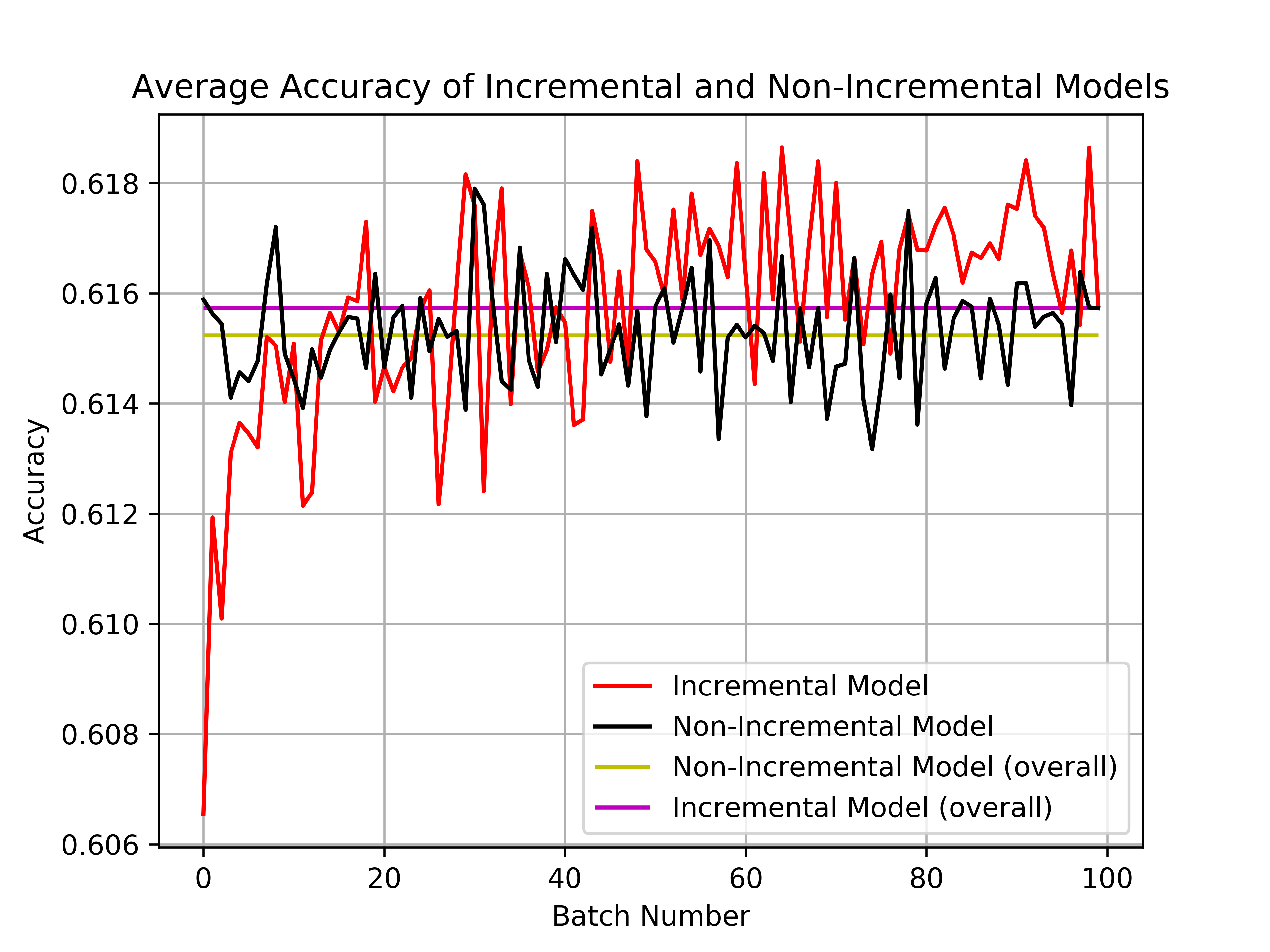
We then compare the average accuracies of the labels produced using our incremental method to the accuracies of the labels produced by an existing off-line source accuracy estimation method based on algorithm 2 [6]. Since this method works in an off-line manner it requires access to the entire set of labels generated by the supervision sources. Using these this method generates its own set of generated labels with which we then calculate the baseline accuracy using the accuracy metric above.
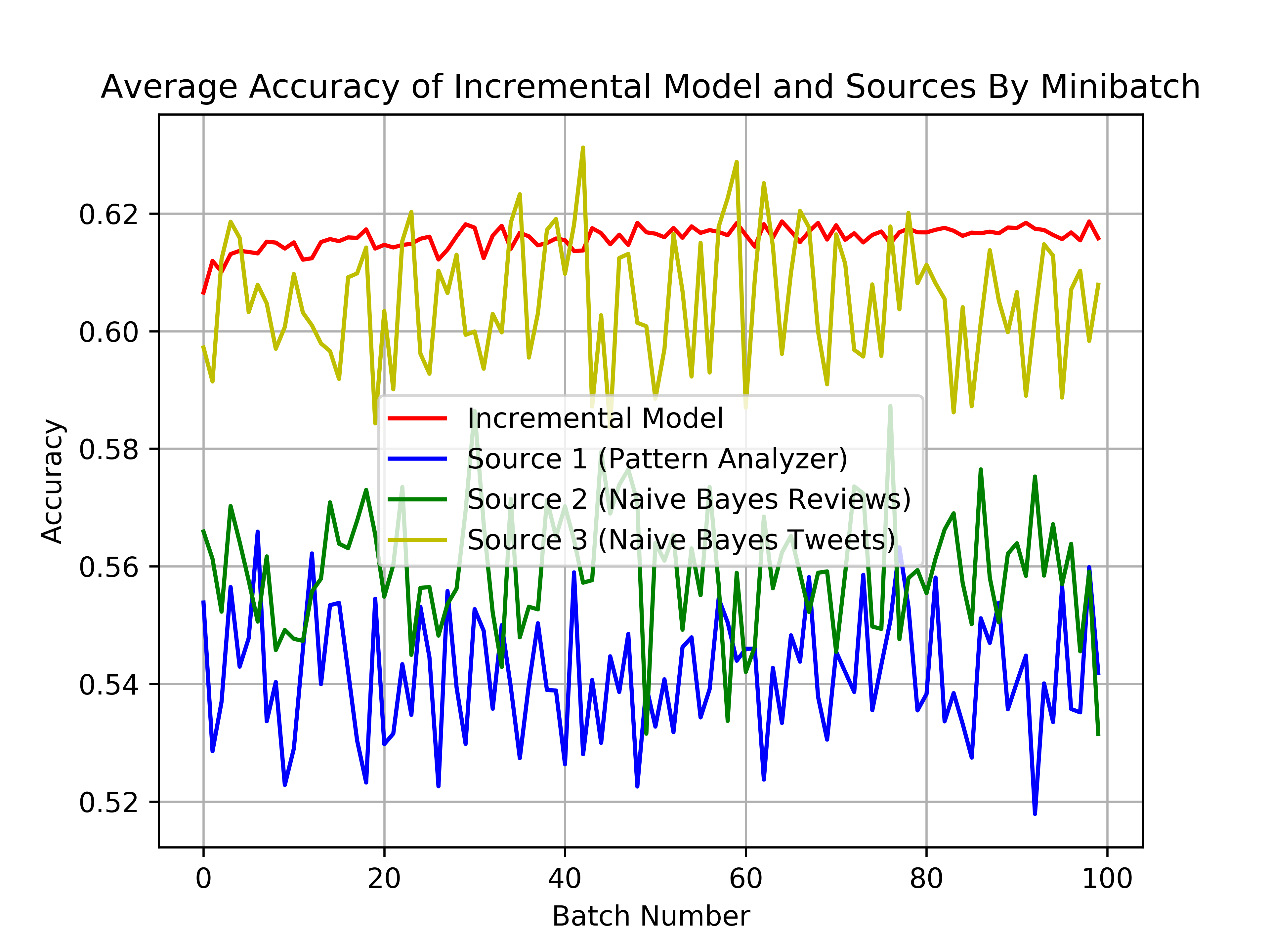
Finally, we compare the accuracy of the labels generated by our method with the accuracy of the labels generated by each of the supervision sources.
Comparing Values of
We then follow the same procedure as above to generate labels for our method, except this time we use different values of .
VI Results
Our tests demonstrate the following:
-
1.
Our model generates labels which are more accurate than those generated by the baseline [when averaged over all 5 tests].
-
2.
Both our method and the baseline generate labels which are more accurate than those generated by each of the supervision sources.
-
3.
Our tests of the accuracy of labels generated by our method using different values of yields an optimal values and shows convexity over the values tested.
Theses tests show that the average accuracy of the incremental model qualitatively appears to increase as the number of samples seen grows. This result is not surprising as we would expect our source accuracy estimate approaches the true accuracy as the number of examples seen increases. This implies that the incremental approach we propose generates more accurate labels as a function of the number of examples seen, unlike the supervision sources which are pre-trained and therefore do not generate more accurate labels as the number of labeled examples grows.
These tests also suggest that an optimal value for for this problem is approximately which is in the interior of the set of values tested for . Since we used minibatches in each test of the incremental model this implies that choosing an which places greater weight on more recent examples yields better performance, although more tests are necessary to make any stronger claims.
Finally, we note that none of the models here tested are in themselves highly-accurate as classification models. This is not unexpected as the supervision sources were intentionally chosen to be ”off-the-shelf” models and no feature engineering was performed on the underlying text data, neither for the datasets used in pre-training the two classifier supervision sources nor for the test set [besides Tf-idf vectorization]. The intention in this test was to compare the relative accuracies of the two generative methods, not to design an accurate discriminative model.
VII Conclusion
We develop an incremental approach for estimating weak supervision source accuracies. We show that our method generates labels for unlabeled data which are more accurate than those generated by pre-existing non-incremental approaches. We frame our specific test case in which we use pre-trained models and heuristic functions as supervision sources as a transfer learning problem and we show that our method generates labels which are more accurate than those generated by the supervision sources themselves.
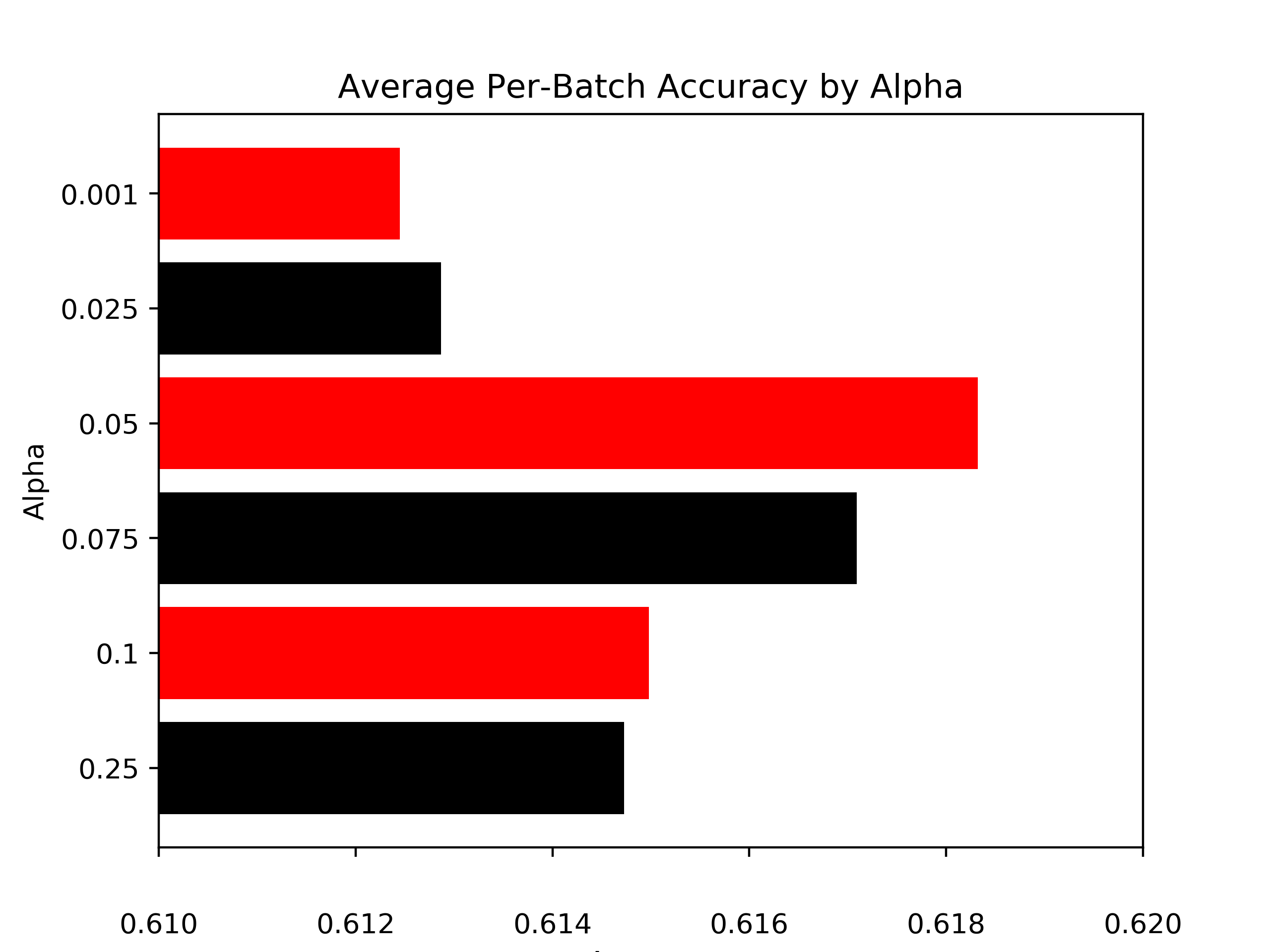
| Alpha | 0.001 | 0.01 | 0.025 | 0.05 | 0.1 | 0.25 |
| Accuracy | 0.61245 | 0.61287 | 0.61832 | 0.61709 | 0.61498 | 0.61473 |
References
- [1] Alexander Ratner. Stephen Bach. Paroma Varma. Chris Ré. (2017) ”Weak Supervision: The New Programming Paradigm for Machine Learning”. Snorkel Blog.
- [2] Mayee Chen. Frederic Sala. Chris Ré. ”Lecture Notes on Weak Supervision”. CS 229 Lecture Notes. Stanford University.
- [3] Paroma Varma. Frederic Sala. Ann He. Alexander Ratner. Christopher Ré. (2019) ”Learning Dependency Structures for Weak Supervision Models”. Preprint.
- [4] Alexander Ratner. Braden Hancock. Jared Dunnmon. Frederic Sala. Shreyash Pandey. Christopher Ré. (2018) ”Training Complex Models with Multi-Task Weak Supervision”. Preprint.
- [5] Emmanuel J. Candès. Xiaodong Li. Yi Ma. John Wright. ”Robust principal component analysis?” Journal of the ACM. Vol 58. Issue 11.
- [6] Alexander Ratner. Stephen H. Bach. Henry Ehrenberg. Jason Fries. Sen Wu. Christopher Ré. ”Snorkel: Rapid Training Data Creation with Weak Supervision.” Preprint.
- [7] Sinno Jialin Pan. Qiang Yang (2009) ”A Survey on Transfer Learning”. IEEE Transactions on Knowledge and Data Engineering. Vol 22. Issue 10.