Weakly Nonlinear Analysis of Peanut-Shaped Deformations for Localized Spots of Singularly Perturbed Reaction-Diffusion Systems
Abstract
Spatially localized 2-D spot patterns occur for a wide variety of two component reaction-diffusion systems in the singular limit of a large diffusivity ratio. Such localized, far-from-equilibrium, patterns are known to exhibit a wide range of different instabilities such as breathing oscillations, spot annihilation, and spot self-replication behavior. Prior numerical simulations of the Schnakenberg and Brusselator systems have suggested that a localized peanut-shaped linear instability of a localized spot is the mechanism initiating a fully nonlinear spot self-replication event. From a development and implementation of a weakly nonlinear theory for shape deformations of a localized spot, it is shown through a normal form amplitude equation that a peanut-shaped linear instability of a steady-state spot solution is always subcritical for both the Schnakenberg and Brusselator reaction-diffusion systems. The weakly nonlinear theory is validated by using the global bifurcation software pde2path [H. Uecker et al., Numerical Mathematics: Theory, Methods and Applications, 7(1), (2014)] to numerically compute an unstable, non-radially symmetric, steady-state spot solution branch that originates from a symmetry-breaking bifurcation point.
1 Introduction
Spatially localized patterns arise in a diverse range of applications including, the ferrocyanide-iodate-sulphite (FIS) reaction (cf. [14], [15]), the chloride-dioxide-malonic acid reaction (cf. [6]), certain electronic gas discharge systems [1], fluid-convection phenomena [10], and the emergence of plant root hair cells mediated by the plant hormone auxin (cf. [2]), among others. One qualitatively novel feature in many of these settings is the observation that spatially localized spot-type patterns can undergo a seemingly spontaneous self-replication process.
Many of these observed localized patterns, most notably those in chemical physics and biology, are modeled by nonlinear reaction-diffusion (RD) systems. In [25], where the two-component Gray-Scott RD model was used to qualitatively model the FIS reaction, full PDE simulations revealed a wide variety of highly complex spatio-temporal localized patterns including, self-replicating spot patterns, stripe patterns, and labyrinthian space-filling curves (see also [27], [19] and [20]). This numerical study showed convincingly that in the fully nonlinear regime a two-component RD system with seemingly very simple reaction kinetics can admit highly intricate solution behavior, which cannot be described by a conventional Turing stability analysis (cf. [31]) of some spatially uniform base state. For certain three-component RD systems in the limit of small diffusivity, Nishiura et. al. (cf. [23], [29]) showed from PDE simulations and a weakly nonlinear bifurcation analysis that a subcritical peanut-shaped instability of a localized radially symmetric spot plays a key role in understanding the dynamics of traveling spot solutions. These previous studies, partially motivated by the pioneering numerical study of [25], have provided the impetus for developing new theoretical approaches to analyze some of the novel dynamical behaviors and instabilities of localized patterns in RD systems in the “far-from-equilibrium” regime [21]. A survey of some novel phenomena and theoretical approaches associated with localized pattern formation problems are given in [36], [21] and [10]. The main goal of this paper is to use a weakly nonlinear analysis to study the onset of spot self-replication for certain two-component RD systems in the so-called “semi-strong” regime, characterized by a large diffusivity ratio between the solution components.
The derivation of amplitude, or normal form, equations using a multi-scale perturbation analysis is a standard approach for characterizing the weakly nonlinear development of small amplitude patterns near bifurcation points. It has been used with considerable success in physical applications, such as in hydrodynamic stability theory and materials science (cf. [5], [38]) and in biological and chemical modeling through RD systems defined in planar spatial domains and on the sphere (cf. [38], [17], [18], [3]). However, in certain applications, the effectiveness of normal form theory is limited owing to the existence of subcritical bifurcations (cf. [3]) or the need for an extreme fine-tuning of the model parameters in order to be within the range of validity of the theory (cf. [43]). In contrast to the relative ease in undertaking a weakly nonlinear theory for an RD system near a Turing bifurcation point of the linearization around a spatially uniform or patternless state, it is considerably more challenging to implement such a theory for spatially localized steady-state patterns. This is owing to the fact that the linearization of the RD system around a spatially localized spot solution leads to a singularly perturbed eigenvalue problem in which the underlying linearized operator is spatially heterogeneous. In addition, various terms in the multi-scale expansion that are needed to derive the amplitude equation involve solving rather complicated spatially inhomogeneous boundary value problems. In this direction, a weakly nonlinear analysis of temporal amplitude oscillations (breathing instabilities) of 1-D spike patterns was developed for a class of generalized Gierer-Meinhardt (GM) models in [37] and for the Gray-Scott and Schnakenberg models in [9]. A criterion for whether these oscillations, emerging from a Hopf bifurcation point of the linearization, are subcritical or supercritical was derived. A related weakly nonlinear analysis for competition instabilities of 1-D steady-state spike patterns for the GM and Schnakenberg models, resulting from a zero-eigenvalue crossing of the linearization, was developed in [16]. Finally, for a class of coupled bulk-surface RD systems, a weakly nonlinear analysis for Turing, Hopf, and codimension-two Turing-Hopf bifurcations of a patterned base-state was derived in [24].
The focus of this paper is to develop and implement a weakly nonlinear theory to analyze branching behavior associated with peanut-shaped deformations of a locally radially symmetric steady-state spot solution for certain singularly perturbed RD systems. Previous numerical simulations of the Schnakenberg and Brusselator RD systems in [13], [28] and [32] (see also [30]) have indicated that a non-radially symmetric peanut-shape deformation of the spot profile can, in certain cases, trigger a fully nonlinear spot self-replication event. The parameter threshold for the onset of this shape deformation linear instability has been calculated in [13] and [28] for the Schnakenberg and Brusselator models, respectively. We will extend this linear theory by using a multi-scale perturbation approach to derive a normal form amplitude equation characterizing the local branching behavior associated with peanut-shaped instabilities of the spot profile. From a numerical evaluation of the coefficients in this amplitude equation we will show that a peanut-shaped instability of the spot profile is always subcritical for both the Schnakenberg and Brusselator models. This theoretical result supports the numerical findings in [13], [28] and [32] that a peanut-shaped instability of a localized spot is the trigger for a fully nonlinear spot-splitting event, and it solves an open problem discussed in the survey article [39].
The dimensionless Schnakenberg model in the two-dimensional unit disk is formulated as
| (1.1) |
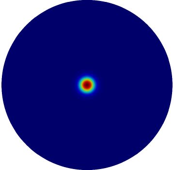
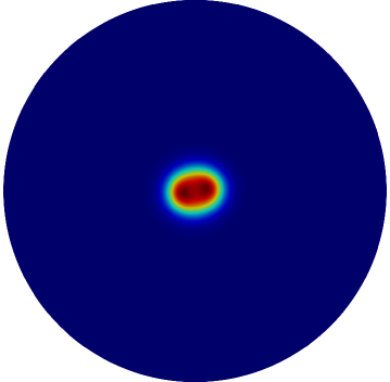
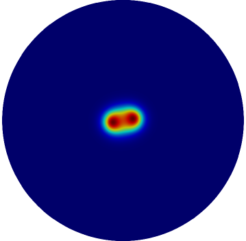
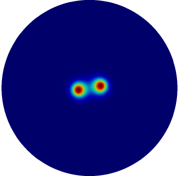
with on . Here , , , and the constant is called the feed-rate. For a spot centered at the origin of the disk, the contour plot in Fig. 1 of at different times, as computed numerically from (1.1), shows a spot self-replication event as the feed-rate is slowly ramped above the threshold value . At this threshold value of the spot profile becomes unstable to a peanut-shaped deformation (see §3 for the linear stability analysis).
Rigorous analytical results for the existence and linear stability of localized spot patterns for the Schnakenberg model (1.1) in the large regime , where , are given in [41] and for the related Gray-Scott model in [40] (see [42] for a survey of such rigorous results). For the regime , a hybrid analytical-numerical approach, which has the effect of summing all logarithmic terms in powers of , was developed in [13] to construct quasi-equilibrium patterns, to analyze their linear stability properties, and to characterize slow spot dynamics. An extension of this hybrid methodology applied to other RD systems was given in [4], [28], [30], [32] and [2], and is surveyed in [39].
We remark that the mechanism underlying the self-replication of 1-D localized patterns is rather different than the more conventional symmetry-breaking mechanism that occurs in 2-D. In a one-dimensional domain, the self-replication behavior of spike patterns has been interpreted in terms of a nearly-coinciding hierarchical saddle-node global bifurcation structure of branches of multi-spike equilibria, together with the existence of a dimple-shaped eigenfunction of the linearization near the saddle-node point (see [22], [8], [7], [12], [35], [11], [19], [27] and the references therein).
The outline of this paper is as follows. For the Schnakenberg RD model (1.1), in §2 we use the method of matched asymptotic expansions to construct a steady-state, locally radially symmetric, spot solution centered at the origin of the unit disk. In §3 we perform a linear stability analysis for non-radially symmetric perturbations of this localized steady-state, and we numerically compute the threshold conditions for the onset of a peanut-shaped instability of a localized spot. Although much of this steady-state and linear stability theory has been described previously in [13], it provides the required background context for describing the new weakly nonlinear theory in §4. More specifically, in §4 we develop and implement a weakly nonlinear analysis to characterize the branching behavior associated with peanut-shaped instabilities of a localized spot. From a numerical evaluation of the coefficients in the resulting normal form amplitude equation we show that a peanut-shaped deformation of a localized spot is subcritical. By using the bifurcation software pde2path [34], the weakly nonlinear theory is validated in §4.1 by numerically computing an unstable non-radially symmetric steady-state spot solution branch that emerges from the peanut-shaped linear stability threshold of a locally radially symmetric spot solution. In §5 we perform a similar multi-scale asymptotic reduction to derive an amplitude equation characterizing the weakly nonlinear development of peanut-shaped deformations of a localized spot for the Brusselator RD model, originally introduced in [26]. From a numerical evaluation of the coefficients in this amplitude equation, which depend on a parameter in the Brusselator reaction-kinetics, it is shown that peanut-shaped linear instabilities are always subcritical. This theoretical result predicting subcriticality is again validated using pde2path [34]. In §6 we summarize a few key qualitative features of our hybrid analytical-numerical approach to derive the amplitude equation, and we discuss a few possible extensions of this work.
2 Asymptotic construction of steady state solution
We use the method of matched asymptotic expansions to construct a steady-state single spot solution centered at in the unit disk. In the inner region near , we set
| (2.2) |
In the inner region, for , the steady-state problem is
| (2.3) |
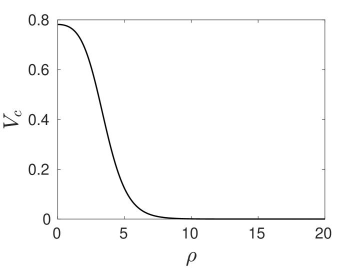
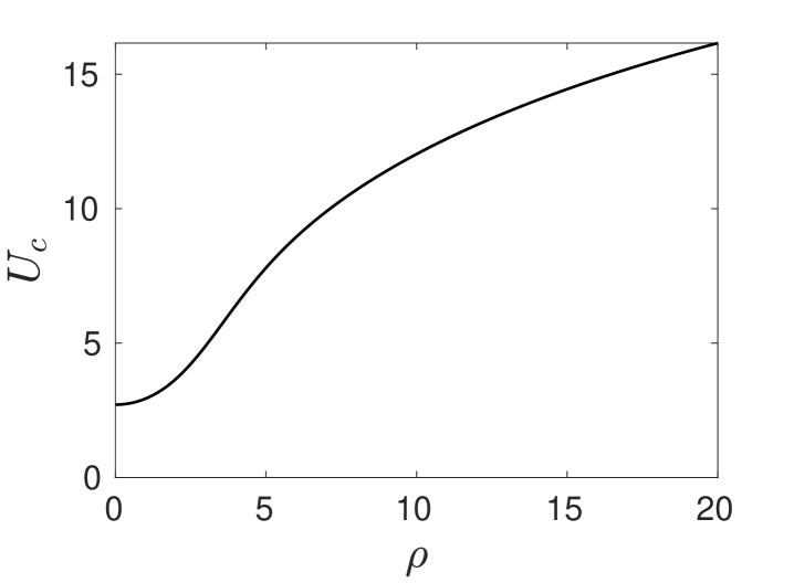
We seek a radially symmetric solution in the form and , where . Upon neglecting the terms, we obtain the core problem
| (2.4) |
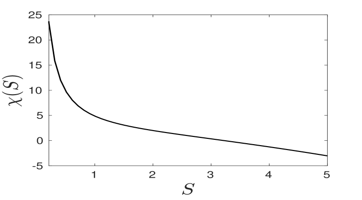
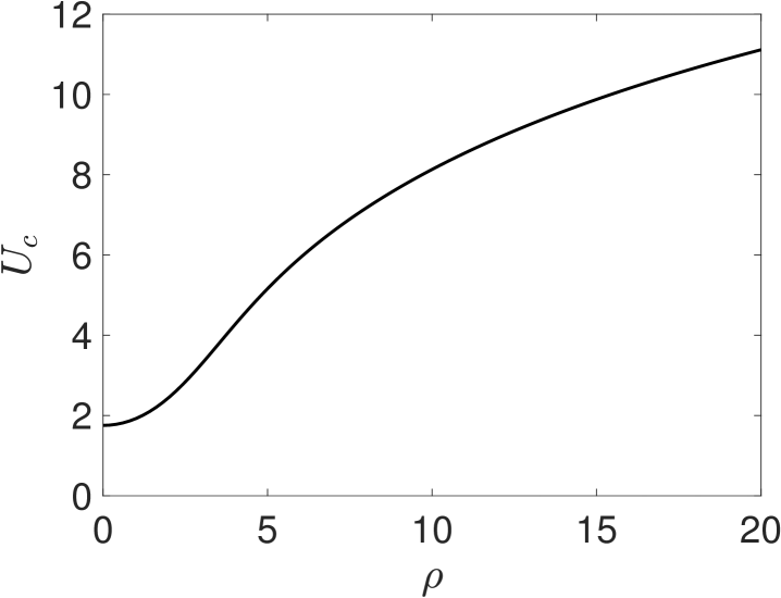
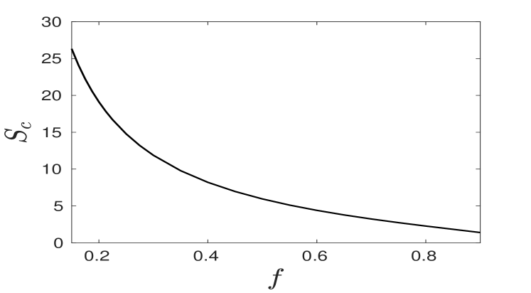
In particular, we must allow to have far-field logarithmic growth whose strength is characterized by the parameter , which will be determined below (see (2.8)) in terms of the feed rate parameter . The term in the far-field behavior depends on , and is denoted by . It must be computed numerically from the BVP (2.4). A plot of the numerically-computed versus is shown in Fig. 2. By integrating the equation in (2.4), we obtain the identity that
| (2.5) |
In the limit , the term in the outer region can be represented, in the sense of distributions, as a Dirac source term using the correspondence rule
| (2.6) |
where (2.5) was used. As a result, the outer problem for in (1.1) is
| (2.7) |
We integrate (2.7) over the disk and use the Divergence theorem and , to get
| (2.8) |
To represent the solution to (2.7) we introduce the Neumann Green’s function for the unit disk, which is defined uniquely by
| (2.9) |
where is the regular part of the Green’s function. The solution to (2.7) is
| (2.10) |
where is a constant to be determined below by asymptotic matching the inner and outer solutions. The Neumann Green’s function with singularity at the origin is
| (2.11) |
Therefore, by using (2.11) in (2.10), the outer solution satisfies
| (2.12) |
By using the far-field behavior of the inner solution in (2.4), we obtain for that
| (2.13) |
From an asymptotic matching of (2.12) and (2.13), we identity as
| (2.14) |
Upon substituting (2.14) and (2.11) into (2.10) we conclude that the outer solution is
| (2.15) |
Remark 2.1
Our asymptotic approximation of matching the core solution to the outer solution effectively sums all the logarithmic term in the expansion in powers of . (see [13] and the references therein). Since the spot is centered at the origin of the unit disk, there is no term in the local behavior near of the outer solution. More specifically, setting , the outer solution (2.15) yields
| (2.16) |
as we approach the inner region, which yields an unmatched term. Together with (2.3), this implies that the steady-state inner solution has the asymptotics and . This estimate is needed below in our weakly nonlinear analysis. In contrast, when a spot is not centered at its steady-state location, the correction to and in the inner expansion is and is determined by the gradient of the regular part of the Green’s function.
3 Linear stability analysis
In this section, we perform a linear stability analysis of the steady-state one-spot solution in the unit disk. For convenience, we will represent a column vector by the notation For a steady-state spot centered at the origin, we will formulate the linearized stability problem in the quarter disk, defined by .
Let be the steady-state spot solution centered at the origin. We introduce the perturbation
| (3.17) |
into (1.1) and linearize. This leads to the singularly perturbed eigenvalue problem
| (3.18) |
with on .
In the inner region near we introduce
| (3.19) |
with . With and , we neglect the terms to obtain the eigenvalue problem
| (3.20) |
where the operator is defined by . We seek eigenfunctions of (5.79) with and as . An unstable eigenvalue of this spectral problem satisfying corresponds to a non-radially symmetric spot-deformation instability.
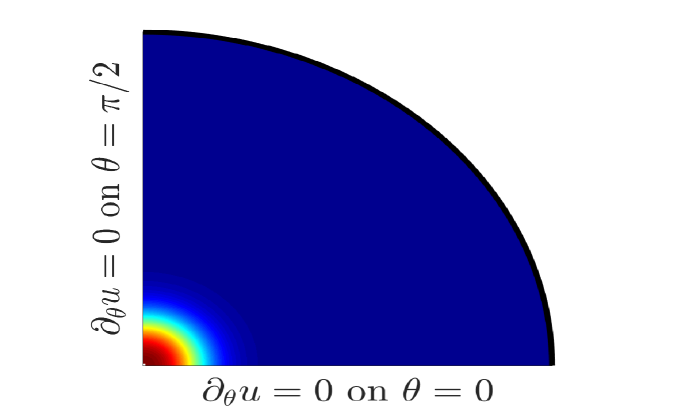
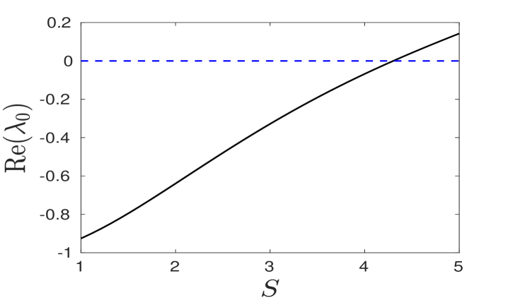
For each angular mode , the eigenvalue of (3.20) with the largest real part is a function of the source strength . To determine we discretize (3.20) as done in [13] to obtain a finite-dimensional generalized eigenvalue problem. We calculate numerically from this discretized problem, with the results shown in the right panel of Fig. 3. In the left panel of Fig. 3 we show the quarter-disk geometry.
For the angular mode , we find that when , which agrees with the result first obtained in [13]. At this critical value of , we define
| (3.21) |
so that there exists a non-trivial solution, labeled by , to
| (3.22) |
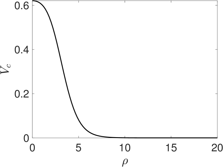
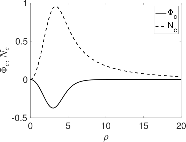
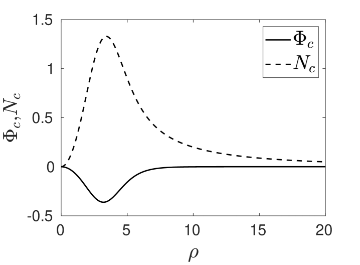
For , we have that exponentially as and as . As such, we impose for . Since (3.22) is a linear homogeneous system, the solution is unique up to a multiplicative constant. We normalize the solution to (3.22) using the condition
| (3.23) |
A plot of the numerically computed inner solution and is shown in Fig. 4.
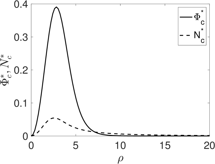
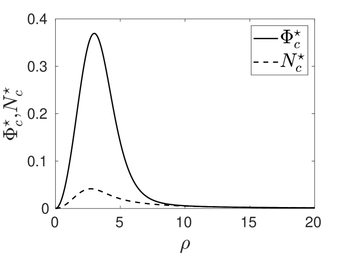
Next, for , it follows that there exists a nontrivial solution to the adjoint problem
| (3.24) |
for which we impose the convenient normalization condition .
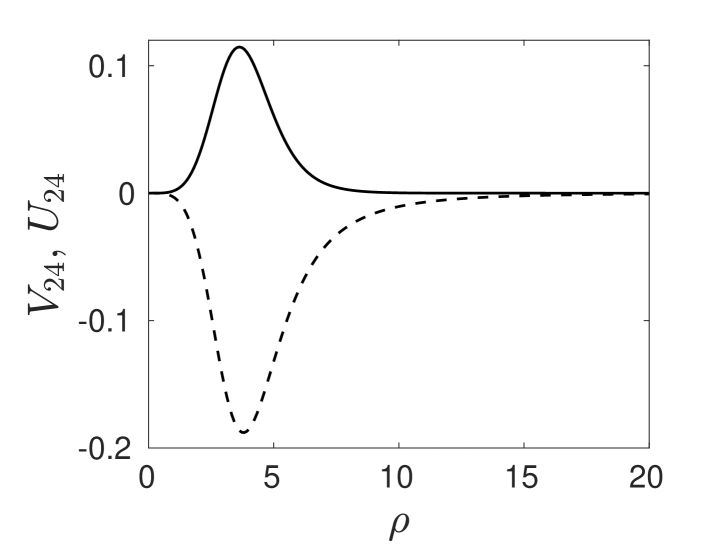
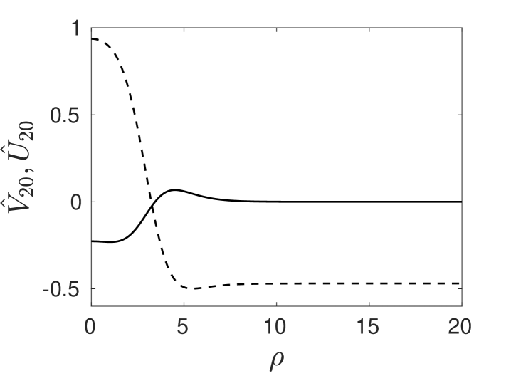
In Fig. 5 we plot the numerically computed nullvector and , satisfying (3.22), as well as the adjoint and , satisfying (3.24).
3.1 Eigenvalue of splitting perturbation theory
In this subsection we calculate the change in the eigenvalue associated with the mode shape deformation when is slightly above . This calculation is needed to clearly identify the linear term in the amplitude equation for peanut-splitting instabilities, as derived below in §4 using a weakly nonlinear analysis.
We denote and as the solution to the core problem (2.4). The linearized eigenproblem associated with the angular mode is given by
| (3.25) |
When , we have and , for which is an eigenvalue in (3.25). We now calculate the change in the eigenvalue when
| (3.26) |
For convenience, we introduce the short hand notation
We first expand the core solution for as
| (3.27) |
so that the perturbation to the matrix is
| (3.28) |
where we write and .
Next, we expand the eigenpair for as
| (3.29) |
We substitute (3.27), (3.28) and (3.29) into (3.25). The terms yield (3.22), while from the terms we obtain that satisfies
| (3.30) |
Upon taking the inner product between (3.30) and the adjoint solution defined in (3.24), we have
| (3.31) |
where we have used By using integration-by-parts twice, the identity , and decay at infinity, we obtain
Together with (3.30), we have derived the solvability condition
| (3.32) |
By solving for , and then rearranging the resulting expression, we obtain that
| (3.33) |
From a numerical quadrature of the integrals in (3.33), which involves the numerical solution to (3.21), (3.22) and (3.24), we calculate that . Therefore, when for we conclude that .
Remark 3.1
As shown in [13] for the Schnakenburg model, as is increased the first non-radially symmetric mode to go unstable is the peanut-splitting mode, which occurs when . Higher modes first go unstable at larger values of , denoted by . From Table 1 of [13], these critical values of are , , and . Since our weakly nonlinear analysis will focus only on a neighbourhood of , the higher modes are all linearly stable in this neighbourhood.
4 Amplitude equation for the Schnakenberg model
In this section we derive the amplitude equation associated with the peanut-splitting linear stability threshold for the Schnakenberg model. This amplitude equation will show that this spot shape-deformation instability is subcritical.
To do so, we first introduce a small perturbation around the linear stability threshold given by , where . In this way, the obtain the Taylor expansion . Then, we introduce a slow time scale . As such, the inner problem in terms of and for is
| (4.34a) | |||
| for which we impose exponentially as , while | |||
| (4.34b) | |||
In (4.34), we expand and as
| (4.35) |
where is the radially symmetry core solution, satisfying (2.4). Furthermore, we assume that
| (4.36) |
so that the terms in (4.34a) are asymptotically smaller than terms of order for .
Remark 4.1
The error in our asymptotic construction is for a spot that is centered at its equilibrium location (see Remark 2.1). We need the scaling assumption (4.36) to ensure that the higher order in approximation of the steady-state is smaller than the approximation error involved in deriving the amplitude equation. For a spot pattern in a quasi-equilibrium state, the error in the construction of the steady-state is , which renders our analysis invalid for quasi-equilibrium patterns. We refer to the discussion section §6 where this issue is elaborated further.
We then substitute (4.35) into (4.34) and collect powers of . From the terms, we obtain that and satisfy
| (4.37a) | ||||
| (4.37b) | ||||
From the far-field condition (4.37b), we can identify that and are the core solution with . In other words, we have
| (4.38) |
From collecting terms, and setting and , we find that satisfies
| (4.39) |
We conclude that is related to the eigenfunction solution to (3.22). We introduce the amplitude function , while writing as
| (4.40) |
Remark 4.2
By collecting terms we readily obtain that on satisfies
| (4.41a) | |||
| where we have defined and by | |||
| (4.41b) | |||
By using (4.40) for and , together with the identity , we can write as
| (4.42) |
This suggests a decomposition of the solution to (4.41a) in the form
| (4.43) |
where the problems for and are formulated below.
Firstly, we define to be the radially symmetric solution to
| (4.44a) | |||
| where , for which we can impose that | |||
| (4.44b) | |||
Next, we define to be the solution to
| (4.45a) | |||
| We can impose exponentially as . As indicated in (4.34b), we have | |||
| (4.45b) | |||
Since as , we must have .
Next, we decompose by first observing that is a radial solution to the homogeneous problem
| (4.46) |
This suggests that it is convenient to introduce the following decomposition to isolate the two sources of inhomogeneity in (4.45):
| (4.47) |
where is taken to be the radial solution to
| (4.48) |
In Appendix A we discuss in detail the derivation of the far-field condition for imposed in (4.48). Moreover, since as , at the end of Appendix A we show how this fact can be accounted for in a simple modification of the outer solution given in (2.15).
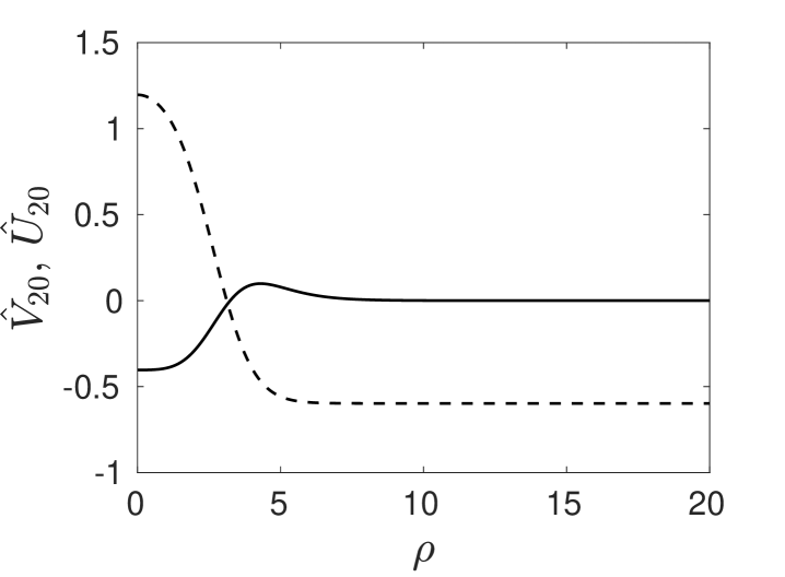
In view of (4.47) and (4.44), the solution to (4.41a), as written in (4.43), is
| (4.49) |
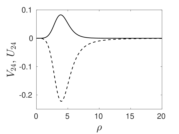
In the left and right panels of Fig. 6 we plot the numerically computed solution to (4.48) and (4.44), respectively.
The solvability condition, which yields the amplitude equation for , arises from the problem. At this order, we find that satisfies
| (4.50a) | |||
| where we have defined and by | |||
| (4.50b) | |||
Upon substituting (4.40) and (4.49) into , we can write in (4.50b) in terms of a truncated Fourier cosine expansion as
| (4.51a) | ||||
| where and are defined by | ||||
| (4.51b) | ||||
| (4.51c) | ||||
| (4.51d) | ||||
In this way, the solution to (4.50a) satisfies
| (4.52) |
where . The right-hand side of this expression suggests that we decompose as
| (4.53a) | ||||
| so that from (4.52) we obtain that and are radial solutions to | ||||
| (4.53b) | ||||
| (4.53c) | ||||
We now impose a solvability condition for the solution to (4.53b). Recall from (3.24) that there is a non-trivial solution to .
so that upon using and , we solve for to obtain
| (4.56) |
By rearranging this expression we conclude that
| (4.57) |
In summary, the normal form of the amplitude equation is given by
| (4.58a) | |||
| where and are given by | |||
| (4.58b) | |||
and and are given in (4.51b) and (4.51c), respectively. By comparing our expression for in (4.58b) with (3.33) we conclude that , where is the eigenvalue for the mode instability, as derived in (3.33) when with . Moreover, from a numerical quadrature we calculate that .
Multiplying both sides of (4.58a) by and using the time scale transformation , the amplitude equation (4.58a) in terms of is
| (4.59) |
Since are numerically found to be positive, the non-zero steady small amplitude in (4.59) exists only when . In this case, we have
| (4.60) |
Remark 4.3
By our assumption , we conclude that our weakly nonlinear analysis is valid only when .
4.1 Numerical validation of the amplitude equation
In this subsection we numerically verify the asymptotic approximation of the steady-state in (4.60) as obtained from our amplitude equation. Our approach is to compute the norm difference between the radially symmetric spot solution and its associated bifurcating solution branch originating from the zero eigenvalue crossing of the peanut-shape instability. To do so, we revisit the expansion scheme (4.35) with and for with . This yields the steady-state prediction
| (4.61) |
with . We also expand the radially symmetric one-spot inner solution for as
| (4.62) |
Let . We define the -function norm in the quarter disk by
Let and . From (4.61) and (4.62), we have
| (4.63) |
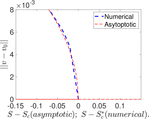
Then, by using the normalization condition (3.23), together with the steady-state amplitude in (4.60), our theoretical prediction from the weakly nonlinear analysis for the non-radially symmetric solution branch is that for , we have
| (4.64) |
where and .
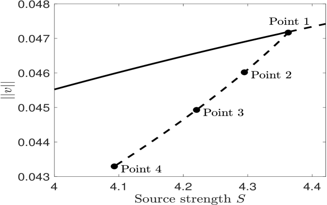
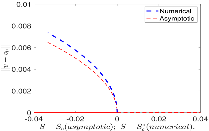
In Fig. 7 we show a favorable comparison of our weakly nonlinear analysis result (4.64) with corresponding full numerical results computed from the steady-state of the Schnakenberg PDE system (1.1) with using the bifurcation software pde2path [34]. The computation is done in the quarter-disk geometry shown in the left panel of Fig. 3. In Fig. 8 we show contour plots, zoomed near the origin, of the non-radially symmetric localized steady-state at four points on the bifurcation diagram in Fig. 7.
(a) 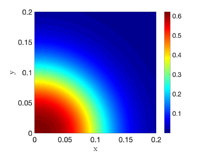 (b)
(b) 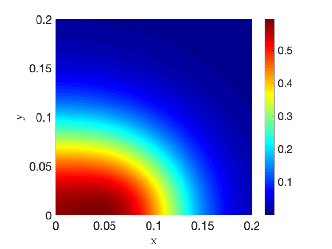
(c) 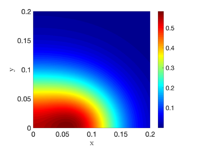 (d)
(d) 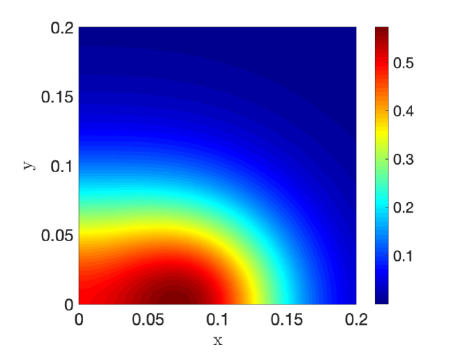
5 Brusselator
We now perform a similar weakly nonlinear analysis for the Brusselator RD model. For this model, it is known that a localized spot undergoes a peanut-shape deformation instability when the source strength exceeds a threshold, with numerical evidence suggesting that this linear instability is the trigger of a nonlinear spot-splitting event (cf. [28], [30], [32]). Our weakly nonlinear analysis will confirm that this peanut-shape symmetry-breaking bifurcation is always subcritical.
The dimensionless Brusselator model in the two-dimensional unit disk is formulated as (cf. [28])
| (5.65) |
with no-flux boundary conditions on . In (5.65) the diffusivity and the feed-rate are positive parameters, while the constant parameter satisfies . Appendix A of [28] provides the derivation of (5.65) starting from the form of the Brusselator model introduced originally in [26].
We first use the method of matched asymptotic expansions to construct a one-spot steady-state solution centered at the origin of the unit disk. In the inner region near we introduce , and by
| (5.66) |
In the inner region, for , the steady-state problem obtained from (5.65) is
| (5.67) |
Seeking a radially symmetric solution in the form and , with , we neglect the terms to obtain the radially symmetric core problem
| (5.68) |
where . We observe that the term , which must be computed numerically, depends on the source strength and the Brusselator parameter , with . By integrating the equation in (5.68) we obtain the identity
| (5.69) |
In the outer region, defined away from an region near the origin, we obtain and that satisfies
| (5.70) |
Writing and , we calculate in the sense of distributions that, for ,
| (5.71) |
where we used (5.69) to obtain the last equality. Hence, upon matching the outer to the inner solution for , we obtain the following outer problem:
| (5.72) |
By integrating (5.72) over and using the Divergence theorem together with we calculate as
| (5.73) |
The solution to (5.72) is given by
| (5.74) |
where . Setting , and using , we obtain that
| (5.75) |
This expression is identical to that derived in (2.16) for the Schnakenberg model, and shows that there is an unmatched term feeding back from the outer to the inner region (see Remark 2.1).
Next, we perform a linear stability analysis. Let denote the steady-state spot solution centered at the origin. We introduce the perturbation
| (5.76) |
into (5.65) and linearize. In this way, we obtain the eigenvalue problem
| (5.77) |
with on . In the inner region near we introduce
| (5.78) |
and . With and , we neglect the terms to obtain the following spectral problem governing non-radially symmetric instabilities of the steady-state spot solution:
| (5.79a) | |||
| Here we have defined | |||
| (5.79b) | |||
We seek eigenfunctions of (5.79) with and as .
Next, we determine the stability threshold for a peanut-shape deformation instability with angular mode . For , the appropriate far-field condition is that exponentially and for . As such, we impose for . We denote as the eigenvalue of (5.79) with the largest real part. Our numerical computations show that for fixed on we have at some , and that for . In Fig. 9 we plot our results for on . These results are consistent with the corresponding thresholds first computed in §3 of [28] at some specific values of . Moreover, as shown in Figure 4 of [28], the peanut-splitting mode is the first mode to lose stability as , or equivalently , is increased. Higher modes lose stability at larger value of . Since in our weakly nonlinear analysis we will only consider the neighbourhood of the instability threshold for the peanut-splitting mode, the higher modes of spot-shape deformation are all linearly stable in this neighborhood.
We denote and by and , and we label as the normalized critical eigenfunction at , which satisfies
| (5.80) |
Likewise, at , there exists a non-trivial normalized solution to the homogeneous adjoint problem
| (5.81) |
where and as . In Fig. 10 we plot the core solution and for . In Fig. 11 we plot the numerically computed eigenfunction (left panel) and adjoint eigenfunction (right panel) when .
5.1 Amplitude equation for the Brusselator model
We now derive the amplitude equation associated with the peanut-splitting linear stability threshold for the Brusselator. Since this analysis is very similar to that for the Schnakenberg model in §4 we only briefly outline the analysis.
We begin by introducing a neighborhood of and a slow time defined by
| (5.82) |
In terms of the inner variables (5.66) and (5.82), we have
| (5.83) |
with exponentially as and
| (5.84) |
We now use an approach similar to that in §4 to derive the amplitude equation for the Brusselator model. We substitute the expansion (4.35) into (5.83) and collect powers of , and we assume that as in (4.36). To leading order in , we obtain that and . The solution of the problem is
| (5.85) |
where is the unknown amplitude and is the eigenfunction of (5.80).
From our assumption that , we can neglect the terms in (5.83) as well as the feedback term in (5.75) arising from the outer solution. In this way, the problem for is given on by
| (5.86) |
Here is given in (5.80). As we have shown in §4, the solution to (5.86) can be conveniently decomposed as
| (5.87) |
where . Here and satisfy
| (5.88a) | ||||
| (5.88b) | ||||
Here is defined by
| (5.89) |
As in §4, we must numerically compute the solutions to (5.88a) and (5.88b). In Fig. 12 we plot these solutions for . We observe from the left panel of Fig. 12 that tends to a nonzero constant for .
Next, by collecting the terms in the weakly nonlinear expansion, we find that satisfies
| (5.90a) | |||
| Here is defined in (5.86), while and are defined by | |||
| (5.90b) | |||
By using the expressions for and from (5.85) and (5.87), respectively, we can obtain a modal expansion of exactly as in (4.51) for the Schnakenberg model. In this way, we obtain (4.52) in which we replace by .
The remainder of the analysis involving the imposition of the solvability condition to derive the amplitude equation exactly parallels that done in §4. We conclude that the amplitude equation associated with peanut-shape deformations of a a spot is
| (5.91a) | |||
| where and , which depend on the Brusselator parameter , are given by | |||
| (5.91b) | |||
Here and are defined in (4.51b) and (4.51c), respectively, in terms of the Brusselator core solution , its eigenfunction satisfying (5.80), and the solutions to (5.88a) and (5.88b).
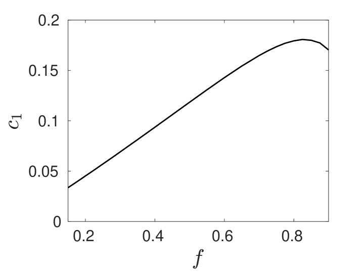
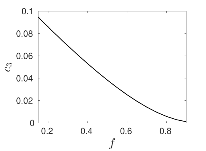
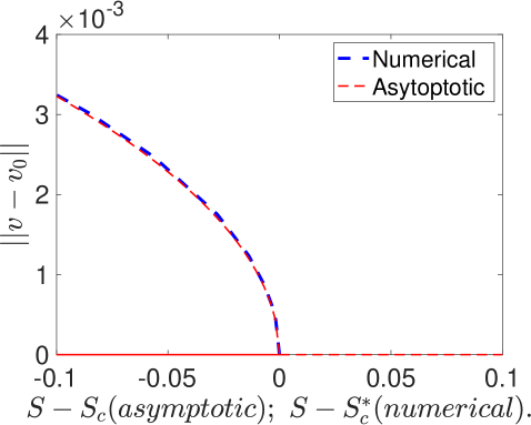
In Fig. 13 we plot the numerically computed coefficients and in the amplitude equation (5.91a) versus the Brusselator parameter on . We observe that both and on this range. This establishes that the peanut-shaped deformation of a steady-state spot is always subcritical, and that the emerging solution branch of non-radially symmetric spot equilibria, which exists only if , is linearly unstable. The steady-state amplitude of this bifurcating non-radially symmetric solution branch is
| (5.92) |
For three values of , in Fig. 14 we favorably compare our weakly nonlinear analysis result (5.92) with corresponding full numerical results computed from the steady-state of the Brusselator (5.65) with in a quarter-disk geometry (see Fig. 3). The full numerical results are obtained using the continuation software pde2path [34], and in Fig. 14 we plot the norm of the deviation from the radiallly symmetric steady state (see (4.63)).

6 Discussion
We have developed and implemented a weakly nonlinear theory to derive a normal form amplitude equation characterizing the branching behavior associated with peanut-shaped non-radially symmetric linear instabilities of a steady-state spot solution for both the Schnakenberg and Brusselator RD systems. From a numerical computation of the coefficients in the amplitude equation we have shown that such peanut-shaped linear instabilities for these specific RD systems are always subcritical. A numerical bifurcation study using pde2path [34] of a localized steady-state spot was used to validate the weakly nonlinear theory, and has revealed the existence of a branch of unstable non-radially symmetric steady-state localized spot solutions. Our weakly nonlinear theory provides a theoretical basis for the observations in [13], [28] and [32] (see also [30]) obtained through full PDE simulations that a linear peanut-shaped instability of a localized spot is the mechanism triggering a fully nonlinear spot self-replication event.
We remark that instabilities resulting from non-radially symmetric shape deformations of a steady-state localized spot solution are localized instabilities, since the associated eigenfunction for shape instabilities decays rapidly away from the center of a spot. As a result, our weakly nonlinear analysis predicting a subcritical peanut-shape instability also applies to steady-state spot patterns of the 2-D Gray-Scott model analyzed in [4], which has the same nonlinear kinetics near a spot as does the Schnakenberg RD system.
However, an important technical limitation of our analysis is that our weakly nonlinear theory is restricted to the consideration of steady-state spot patterns, and does not apply to quasi-equilibrium spot patterns where the centers of the spots evolve dynamically on asymptotically long time intervals towards a steady-state spatial configuration of spots. For such quasi-equilibrium spot patterns there is a non-vanishing feedback from the outer solution that results from the interaction of a spot with the domain boundary or with the other spots in the pattern. This feedback term then violates the asymptotic ordering of the correction terms in our weakly nonlinear perturbation expansion. For steady-state spot patterns there is an asymptotically smaller feedback from the outer solution, and so our weakly nonlinear analysis is valid for , under the assumption that (see Remark 2.1). Here is the spot source strength at which a zero-eigenvalue crossing occurs for a small peanut-shaped deformation of a localized spot. In contrast, for a quasi-equilibrium spot pattern, it was shown for the Schnakenburg model in §2.4 of [13] that, when , the direction of the bulge of a peanut-shaped linear instability is perpendicular to the instantaneous direction of motion of a spot. This result was based on a simultaneous linear analysis of mode (translation) and mode (peanut-shape) localized instabilities near a spot. The full PDE simulations in [13] indicate that this linear instability triggers a fully nonlinear spot-splitting event where the spot undergoes a splitting process in a direction perpendicular to its motion. To provide a theoretical understanding of this phenomena it would be worthwhile to extend this previous linear theory of [13] for quasi-equilibrium spot patterns to the weakly nonlinear regime.
Although our weakly nonlinear theory of spot-shape deformation instabilities has only been implemented for the Schnakenberg and Brusselator RD systems, the hybrid analytical-numerical theoretical framework presented herein applies more generally to other reaction kinetics where a localized steady-state spot solution can be constructed. It would be interesting to determine whether one can identify other RD systems where the branching is supercritical, thereby allowing for the existence of linearly stable non-radially symmetric localized spot steady-states.
In another direction, for the Schnakenberg model in a 3-D spatial domain, it was shown recently in [33] through PDE simulations that a peanut-shaped linear instability is also the trigger for a nonlinear spot self-replication event. It would be worthwhile to extend our 2-D weakly nonlinear theory to this more intricate 3-D setting.
7 Acknowledgements
Tony Wong was supported by a UBC Four-Year Graduate Fellowship. Michael Ward gratefully acknowledges the financial support from the NSERC Discovery Grant program. The authors would like to thank Frédéric Paquin- Lefebvre for some insightful discussions.
Appendix A Far-field condition for for the Schnakenberg model
We derive the far-field condition for used in (4.48) in the derivation of the amplitude equation for peanut-splitting instabilities for the Schnakenberg model. We first observe that the second component of (4.48) satisfies
| (A.1) |
where is defined in (4.42) and where primes indicate derivatives in . For , we have from the first equation in (4.48) that with as . This yields the asymptotic decay behavior
| (A.2) |
for some . As such, we impose at in solving (4.48) numerically. The constant in (A.2) can be calculated from the limit . Our numerical solution of the BVP problem (4.48) with yields .
To find the asymptotic behavior for in (A.1) we decompose it into homogeneous and inhomogeneous parts as
| (A.3a) | |||
| where and satisfies | |||
| (A.3b) | |||
We first estimate for . By using (A.2) for , and using the dominant balance ansatz , we obtain that (A.3b) transforms exactly to
| (A.4) |
To estimate the asymptotic behavior of we apply the method of dominant balance. The appropriate balance for is found to be , which yields
| (A.5) |
Our leading-order balance is self-consistent since we have for . By integrating in (A.5), we get
| (A.6) |
Therefore, we have
| (A.7) |
for some constant . By differentiating the ansatz , followed by using the estimates (A.5) and (A.7), we obtain
| (A.8) |
As a result, we conclude for the homogeneous solution that
| (A.9) |
Next, we consider the particular solution satisfying (A.3b). We use the far field behavior , , , and for , to deduce from (5.89) that
| (A.10) |
Therefore, from (A.3b), for the particular solution satisfies
| (A.11) |
By balancing the first and third terms in this expression we get
| (A.12) |
From this expression, we readily derive that
| (A.13) |
This shows that exponentially as . Upon combining this result with (A.9) we conclude that
| (A.14) |
This dominant balance analysis justifies our imposition of the homogeneous Neumann far-field condition for in (4.48) for the Schnakenberg model. An identical argument can be performed to justify the far-field condition in (5.88a) for the Brusselator model.
From our numerical computation of from (4.48), shown in Fig. 6, we observe that as . We now show how this non-vanishing limit can be accounted for in a modified outer solution. From (4.35) we have for that
| (A.15) |
where from (4.40), while from (4.43) and (4.47). Since as , while and as , we obtain that the far-field behavior of is
| (A.16) |
which specifies the term in (4.34b). Since and from (2.8), the modified outer solution has the form
| (A.17) |
where, in the unit disk , satisfies
| (A.18a) | ||||
| (A.18b) | ||||
where . To complete the expansion in (A.17) we solve (A.18) to get
| (A.19) |
In this way, the non-vanishing limiting behavior of as leads to only a simple modification of the outer solution as given in (2.15).
Finally, we remark that an identical modification of the outer expansion for the Brusselator model can be done when deriving the amplitude equation for peanut-shaped instability of a localized spot.
References
- [1] Y. A. Astrov, H. G. Purwins, Spontaneous division of dissipative solitons in a planar gas-discharge system with high ohmic electrode, Phys. Lett. A, 358(5-6), (2006), pp. 404–408.
- [2] D. Avitabile, V. Brena-Medina, M. J. Ward, Spot dynamics in a plant hair initiation model, SIAM J. Appl. Math., 78(1), (2018), pp. 291–319.
- [3] T. K. Callahan, Turing patterns with O(3) symmetry, Physica D, 188(1), (2004), pp. 65–91.
- [4] W. Chen, M. J. Ward, The stability and dynamics of localized spot patterns in the two-dimensional Gray-Scott model, SIAM J. Appl. Dyn. Sys., 10(2), (2011), pp. 582–666.
- [5] M. Cross, P. Hohenburg, Pattern formation outside of equilibrium, Rev. Mod. Physics, 65, (1993), pp. 851-1112.
- [6] P. W. Davis, P. Blanchedeau, E. Dullos and P. De Kepper (1998), Dividing blobs, chemical flowers, and patterned islands in a reaction-diffusion system, J. Phys. Chem. A, 102(43), pp. 8236–8244.
- [7] A. Doelman, R. A. Gardner, T. J. Kaper, Stability analysis of singular patterns in the 1D Gray-Scott model: A matched asymptotics approach, Physica D, 122(1-4), (1998), pp. 1-36.
- [8] S. Ei, Y. Nishiura, K. Ueda, splitting or edge splitting?: A manner of splitting in dissipative systems, Japan. J. Indus. Appl. Math., 18, (2001), pp. 181-205.
- [9] D. Gomez, L. Mei, J. Wei, Stable and unstable periodic spiky solutions for the Gray-Scott system and the Schnakenberg system, to appear, J. Dyn. Diff. Eqns. (2020).
- [10] E. Knobloch, Spatial localization in dissipative systems, Annu. Rev. Cond. Mat. Phys., 6, (2015), pp. 325–359.
- [11] T. Kolokolnikov, M. Ward, J. Wei, The stability of spike equilibria in the one-dimensional Gray-Scott model: the pulse-splitting regime, Physica D, 202(3-4), (2005), pp. 258–293.
- [12] T. Kolokolnikov, M. J. Ward, J. Wei, Pulse-splitting for some reaction-diffusion systems in one-space dimension, Studies in Appl. Math., 114(2), (2005), pp. 115–165.
- [13] T. Kolokolnikov, M. J. Ward, J. Wei, Spot self-replication and dynamics for the Schnakenberg model in a two-dimensional domain, J. Nonlinear Sci., 19(1), (2009), pp. 1–56.
- [14] K. J. Lee, W. D. McCormick, J. E. Pearson, H. L. Swinney, Experimental observation of self-replicating spots in a reaction-diffusion system, Nature, 369, (1994), pp. 215-218.
- [15] K. J. Lee, H. Swinney, Lamellar structures and self-replicating spots in a reaction-diffusion system, Phys. Rev. E, 51(3), (1995), pp. 1899–1915.
- [16] F. Paquin-Lefebvre, T. Kolokolnikov, M. J. Ward, Competition instabilities of pulse patterns for the 1-d Gierer-Meinhardt model are subcritical, to be submitted, SIAM J. Appl. Math., (2020).
- [17] P. C. Matthews, Transcritical bifurcation with symmetry, Nonlinearity, 16(4), (2003), pp. 1449–1471.
- [18] P. C. Matthews, Pattern formation on a sphere, Phys. Rev. E., 67(3), (2003), pp. 036206.
- [19] C. Muratov, V. V. Osipov, Static spike autosolitons in the Gray-Scott model, J. Phys. A: Math Gen. 33, (2000), pp. 8893–8916.
- [20] C. Muratov, V. V. Osipov, Spike autosolitons and pattern formation scenarios in the two-dimensional Gray-Scott model, Eur. Phys. J. B. 22, (2001), pp. 213–221.
- [21] Y. Nishiura, Far-from equilibrium dynamics, translations of mathematical monographs, Vol. 209, (2002), AMS Publications, Providence, Rhode Island.
- [22] Y. Nishiura, D. Ueyama, A skeleton structure of self-replicating dynamics, Physica D, 130(1-2), (1999), pp. 73-104.
- [23] , Y. Nishiura, T. Teramoto, K. I. Ueda, Scattering of traveling spots in dissipative systems, Chaos 15(4), 047509 (2005).
- [24] F. Paquin-Lefebrve, W. Nagata, M. J. Ward, Pattern formation and oscillatory dynamics in a 2-d coupled bulk-surface reaction-diffusion system, SIAM J. Appl. Dyn. Sys., 18(3), (2019), pp. 1334-1390.
- [25] J. E. Pearson, Complex patterns in a simple system, Science, 216, (1993), pp. 189–192.
- [26] I. Prigogine, R. Lefever, Symmetry breaking instabilities in dissipative systems. II, J. Chem. Physics, 48, (1968), pp. 1695.
- [27] W. N. Reynolds, S. Ponce-Dawson, J. E. Pearson, Self-replicating spots in reaction-diffusion systems, Phys. Rev. E, 56(1), (1997), pp. 185-198.
- [28] I. Rozada, S. Ruuth, M. J. Ward, The stability of localized spot patterns for the Brusselator on the sphere, SIAM J. Appl. Dyn. Sys., 13(1), (2014), pp. 564–627.
- [29] T. Teramoto, K. Suzuki, Y. Nishiura, Rotational motion of traveling spots in dissipative systems, Phys. Rev. E. 80(4):046208, (2009).
- [30] P. Trinh, M. J. Ward, The dynamics of localized spot patterns for reaction-diffusion systems on the sphere, Nonlinearity, 29(3), (2016), pp. 766–806.
- [31] A. Turing, The chemical basis of morphogenesis, Phil. Trans. Roy. Soc. B, 327, (1952), pp. 37–72.
- [32] J. Tzou, M. J. Ward, Effect of open systems on the existence, stability, and dynamics of spot patterns in the 2D Brusselator model, Physica D, 373, (2018), pp. 13–37.
- [33] J. Tzou, S. Xie, T. Kolokolnikov, M. J. Ward, The stability and slow dynamics of localized spot patterns for the 3D Schnakenberg reaction-diffusion model, SIAM J. Appl. Dyn. Sys., 16(1), (2017), pp. 294–336.
- [34] H. Uecker, D. Wetzel, J. D. Rademacher, Pde2path-A Matlab package for continuation and bifurcation in 2D elliptic systems, Numerical Mathematics: Theory, Methods and Applications, 7(1), (2014), pp. 58–106.
- [35] D. Ueyama, Dynamics of self-replicating patterns in the one-dimensional Gray-Scott model, Hokkaido Math J., 28(1), (1999), pp. 175-210.
- [36] V. K. Vanag, I. R. Epstein, Localized patterns in reaction-diffusion systems, Chaos 17(3), 037110, (2007).
- [37] F. Veerman, Breathing pulses in singularly perturbed reaction-diffusion systems, Nonlinearity, 28, (2015), pp. 2211-2246.
- [38] D. Walgraef, Spatio-temporal pattern formation, with examples from physics, chemistry, and materials science, in book series, Partially ordered systems, Springer, New York, (1997), 306 p.
- [39] M. J. Ward, Spots, traps, and patches: asymptotic analysis of localized solutions to some linear and nonlinear diffusive processes, Nonlinearity, 31(8), (2018), R189 (53 pages).
- [40] J. Wei, M. Winter, Existence and stability of multiple spot solutions for the Gray-Scott model in , Physica D, 176(3-4), (2003), pp. 147-180.
- [41] J. Wei, M. Winter, Stationary multiple spots for reaction-diffusion systems, J. Math. Biol., 57(1), (2008), pp. 53–89.
- [42] J. Wei, M. Winter, Mathematical aspects of pattern formation in biological systems, Applied Mathematical Science Series, Vol. 189, Springer, (2014).
- [43] R. Wittenberg, P. Holmes, The limited effectiveness of normal forms: a critical review and extension of local bifurcation studies of the Brusselator PDE, Physica D, 100(1-2), (1997), pp. 1–40.