Weakly Supervised Regression with Interval Targets

Xin Cheng Yuzhou Cao Ximing Li Bo An Lei Feng

Abstract

This paper investigates an interesting weakly supervised regression setting called regression with interval targets (RIT). Although some of the previous methods on relevant regression settings can be adapted to RIT, they are not statistically consistent, and thus their empirical performance is not guaranteed. In this paper, we provide a thorough study on RIT. First, we proposed a novel statistical model to describe the data generation process for RIT and demonstrate its validity. Second, we analyze a simple selection method for RIT, which selects a particular value in the interval as the target value to train the model. Third, we propose a statistically consistent limiting method for RIT to train the model by limiting the predictions to the interval. We further derive an estimation error bound for our limiting method. Finally, extensive experiments on various datasets demonstrate the effectiveness of our proposed method.

Machine Learning, ICML

1 Introduction

Regression is a significantly important task in machine learning and statistics (Stulp & Sigaud, 2015; Uysal & Güvenir, 1999). The goal of the regression task is to learn a predictive model from a given set of training examples, where each training example consists of an instance (or feature vector) and a real-valued target. Conventional supervised regression normally requires a vast amount of labeled data to learn an effective regression model with excellent performance. However, it could be difficult to obtain fully supervised training examples due to the high cost of data labeling in real-world applications. To alleviate this problem, many weakly supervised regression settings have been investigated, such as semi-supervised regression (Li et al., 2017; Wasserman & Lafferty, 2007; Kostopoulos et al., 2018), multiple-instance regression (Amar et al., 2001; Wang et al., 2011; Park et al., 2020), uncoupled regression (Carpentier & Schlüter, 2016; Xu et al., 2019), and regression with noisy targets (Ristovski et al., 2010; Hu et al., 2020).

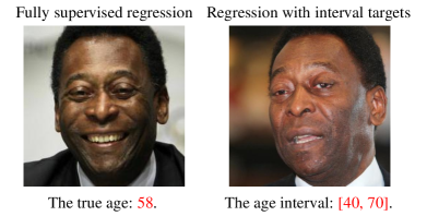
This paper investigates another interesting weakly supervised regression setting called regression with interval targets (RIT). For RIT, we aim to learn a regression model from weakly supervised training examples, each annotated with only an interval that contains the true target value. The learned regression model in this setting is expected to predict the target value of any test instance as accurately as possible. In many real-world scenarios, it is difficult to collect the exact true target value, while it could be easy to provide an interval in which the true target value is contained. A typical example is facial age estimation (Geng et al., 2013). In Figure 1, there are two photos of Ballon d’Or King Pele at the age of 58. The fully supervised regression task requires the exact age of Pele, which is quite difficult to provide because it is common for a person to look the same over a long period of time. However, we can easily get an age interval that contains the true age of Pele. Based on the facial wrinkles, we can determine that the true age is at least 40 but not more than 70. In reality, many regression tasks face this challenge (especially in size/length/age estimation), where it is costly or impossible to obtain a true target value.

Refer to caption — Figure 1: An example of facial age estimation. Both photos were taken when Pele was 58 years old.

Our studied RIT is highly related to interval-valued data prediction (IVDP) (Ishibuchi & Tanaka, 1991; Neto & De Carvalho, 2008, 2010; Fagundes et al., 2014). IVDP allows each training example to be annotated with an interval and learns a regression model to predict the interval containing the true target value of a test instance. There are even some studies that allow features to be intervals as well (Manski & Tamer, 2002; Yang & Liu, 2018; Sadeghi et al., 2019). It is worth noting that IVDP aims to predict the interval that contains the target value, while our studied RIT aims to predict the true target value. Although some of the above methods could be adapted to our studied RIT settings, they are not statistically consistent (i.e., the learned model is infinite-sample consistent to the optimal model), and thus the empirical performance is not guaranteed.

In this paper, we provide a thorough study on RIT, and the main contributions can be summarized as follows:

•

We propose a novel statistical model to describe the data generation process for RIT and demonstrate its validity. Having an explicit data distribution helps us understand how data with interval targets are generated.
•

We analyze a simple selection method for RIT, which selects a particular value in the interval as the target value to train the model. We show that this intuitive method could work well if the middlemost value in the interval is taken as the target value.
•

We propose a statistically consistent limiting method for RIT to train the model by limiting the predictions of the model to the interval. We further derive an estimation error bound for our limiting method.

Extensive experiments on various datasets demonstrate the effectiveness of our proposed method.

2 Related Work

Regression. For the ordinary regression problem, let the feature space be $\mathcal{X}\in\mathbb{R}^{d}$ and the label space be $\mathcal{Y}\in\mathbb{R}$ . Let us denote by $(\bm{x},y)$ an example including an instance $x$ and a real-valued true label $y$ . Each example $(\bm{x},y)\in\mathcal{X}\times\mathcal{Y}$ is assumed to be independently sampled from an unknown data distribution with probability density $p(\bm{x},y)$ . For the regression task, we aim to learn a model $f:\mathcal{X}\mapsto\mathbb{R}$ that tries to minimize the following expected risk:

\displaystyle R(f)=\mathbb{E}_{p(\bm{x},y)}[\ell(f(\bm{x}),y)],

(1)

where $\mathbb{E}_{p(\bm{x},y)}$ denotes the expectation over the distribution $p(\bm{x},y)$ and $\ell:\mathbb{R}\times\mathbb{R}\mapsto\mathbb{R}_{+}$ is a conventional loss function (such as mean squared error and mean absolute error) for regression, which measures how well a model estimates a given real-valued label.

Interval-valued data prediction. In order to consider multiple types of data, such as intervals, weights, and characters, symbolic data analysis (Bock & Diday, 1999; Billard, 2006) has been extensively investigated. As a specific task of symbolic data analysis, the purpose of interval-valued data prediction (IVDP) is to learn an interval predictor from training data annotated with intervals. The challenge of IVDP is mainly to construct a model that outputs intervals (to ensure that the interval holds, e.g., $[0,10]$ instead of $[10,0]$ ). In statistics, Billard & Diday (2000) introduced a central tendency for interval data. (Lauro & Palumbo, 2000) introduced principal component analysis methods for interval data. In addition, by designing proper loss functions, network structures, or output constraints, neural networks can also be trained to output intervals for IVDP (Neto & De Carvalho, 2008, 2010; Giordani, 2015; Yang et al., 2019; Sadeghi et al., 2019).

Regression with interval-censored data. Another related setting is regression with interval-censored data (RICD) (Rabinowitz et al., 1995; Lindsey & Ryan, 1998; Lesaffre et al., 2005; Sun, 2006), which aims to learn a survival function from interval-censored data. In a sequence of time points, a specific event (e.g., machine breakdown, disease attack, death) occurs between two time points, and the interval formed by these two time points is called interval censoring. RICD was widely used in survival analysis (Machin et al., 2006; Kleinbaum et al., 2012; Wang et al., 2019b). In contrast to our studied RIT setting, RICD aims to obtain a survival function to estimate the occurring probability of an event, instead of learning a predictive model.

3 Regression with Interval Targets

Notations. Suppose the given training set is denoted by $\{(\bm{x}_{i},S_{i})\}_{i=1}^{n}$ where $S_{i}$ represents the interval $[\underline{y}_{i},\overline{y}_{i}]\in\mathcal{Y}\times\mathcal{Y}$ assigned to the instance $\bm{x}\in\mathcal{X}$ , and $|S_{i}|=\overline{y}_{i}-\underline{y}_{i}$ represents the size of the interval $S_{i}$ . Each training example $(\bm{x}_{i},S_{i})$ is assumed to be sampled from an unknown joint distribution with probability density $\tilde{p}(\bm{x},S)$ . In this setting, the true label $y_{i}\in\mathcal{Y}$ of the instance $\bm{x}_{i}$ is guaranteed to be contained in the interval $S_{i}$ . The goal of interval regression is to induce a regression model $f:\mathcal{X}\mapsto\mathbb{R}$ that can accurately predict the target value of a test instance. Interestingly, this setting can be considered as a generalized setting of ordinary regression, because we can easily convert the ordinary regression example $(\bm{x}_{i},y_{i})$ to an interval regression example by rewriting $y_{i}$ as the interval $[\underline{y}_{i},\overline{y}_{i}]$ where $\underline{y}_{i}=\overline{y}_{i}=y_{i}$ . In this paper, we denote by $p(\cdot)$ the probability density and $\mathrm{Pr}[\cdot]$ the occurring probability.

Small ambiguity degree. For ensuring that RIT is learnable (i.e., the true target value concealed in the interval is distinguishable), we assume that RIT should satisfy the small ambiguity degree condition (Cour et al., 2011), where the ambiguity degree in our setting is defined as

\displaystyle\lambda=\sup_{(\bm{x},y)\sim p(\bm{x},y),(\bm{x},S)\sim\tilde{p}(\bm{x},S),y^{\prime}\in\mathcal{Y},y^{\prime}\neq y}\mathrm{Pr}[y^{\prime}\in S].

The ambiguity degree $\lambda$ is the maximum probability of a specific incorrect target $y^{\prime}$ co-occurring with the true target $y$ in the same interval $S$ . We can observe that when $\lambda=1$ , the incorrect target $y^{\prime}$ always appears with the true target $y$ together, and thus we can no longer distinguish which one is the true target. Therefore, the RIT setting requires to assume that the small ambiguity degree condition is satisfied (i.e., $\lambda<1$ ), in order to ensure that this setting is learnable.

3.1 Data Generation Process

To avoid the sampled intervals being unreasonable (i.e., the size is unexpectedly large), we use $q$ to denote the maximum allowed interval size $|S|$ . Then, we assume that each example $(\bm{x},S)$ with $S=[\underline{y},\overline{y}]$ is independently sampled from a probability distribution with the following density:

\displaystyle\tilde{p}(x,S)=\int_{\underline{y}}^{\overline{y}}p(S|y)p(\bm{x},y)\mathrm{d}y,

(2)

where

\displaystyle p(S|y)=\left\{\begin{aligned} \frac{2}{q^{2}}&,\quad y\in S\ \mathrm{and}\ |S|\leq q,\\ 0&,\quad\mathrm{otherwise}.\end{aligned}\right.

(3)

In Eq. (2), we assume $p(S|y,\bm{x})=p(S|y)$ , which means that given the true label $y$ , the interval $S$ is independent of the instance $\bm{x}$ . Such a class-dependent and instance-independent assumption was widely adopted by many previous studies in the weakly supervised learning field (Patrini et al., 2017; Ishida et al., 2019; Feng et al., 2020). In Eq. (3), we assume that given a specific label $y$ , all possible intervals $\{S|y\in S,|S|\leq q\}$ are uniformly sampled.

We show that our presented joint distribution $\tilde{p}(\bm{x},S)$ is a valid probability distribution by the following theorem.

Theorem 3.1.

The following equality holds:

\int_{\mathcal{S}}\int_{\mathcal{X}}\tilde{p}(\bm{x},S)\mathrm{d}\bm{x}\mathrm{d}S=1.

(4)

In addition to proving that $\tilde{p}(\bm{x},S)$ is a valid probability distribution, we also need to verify that $\tilde{p}(\bm{x},S)$ meets the key requirement of RIT, i.e., the true target $y$ is guaranteed to be contained in the interval $S$ for every example $(\bm{x},S)$ sampled from $\tilde{p}(\bm{x},S)$ . The following theorem provides an affirmative answer to this question.

Theorem 3.2.

For any interval example $(\bm{x},S)$ independently sampled from the assumed data distribution $\tilde{p}(\bm{x},S)$ defined in Eq. (2), the true target $y$ is always in the interval $S$ , i.e., $\mathrm{Pr}[y\in S|\bm{x},S]=1$ , $\forall(\bm{x},S)\backsim\tilde{p}(\bm{x},S)$ .

3.2 Real-World Motivation

Here, we give a real-world motivation for the assumed data distribution $\tilde{p}(\bm{x},S)$ . For the data annotations in the regression task, it could be difficult to directly provide the exact true target value for each instance. Fortunately, it would be easier if the annotation system can randomly generate an interval and ask annotators whether the true target value is contained in the generated interval or not. Given an instance $\bm{x}$ , the maximum size $q$ of the interval, and the maximum and minimum values $y_{\mathrm{max}},y_{\mathrm{min}}$ of the label space $\mathcal{Y}$ , suppose the annotation system randomly and uniformly samples $\underline{y}$ and $\overline{y}$ from the interval $[y_{\mathrm{min}}-q,y_{\mathrm{max}}+q]$ ( $\pm q$ is to ensure that all possible $y$ have the same possible number of intervals) to generate an interval $S=[\underline{y},\overline{y}]$ . If the sampled $\underline{y}$ and $\overline{y}$ satisfy the two conditions: $\overline{y}-\underline{y}\leq q$ and the true target value $y$ of $\bm{x}$ belongs to $[\underline{y},\overline{y}]$ i.e., $y\in[\underline{y},\overline{y}]$ , then we collect an interval regression example $(\bm{x},S)$ where $S=[\underline{y},\overline{y}]$ , otherwise we discard the interval $S$ for the instance $\bm{x}$ . In this way, each collected interval regression example $(\bm{x},S)$ exactly follows the data distribution defined in Eq. (2). We will demonstrate this argument below.

We start by considering the case where the annotation system has discarded all intervals larger than a given maximum interval value $q$ . Then we have the following lemma.

Lemma 3.3.

Given the maximum value $q$ allowed for the interval size, and the maximum value $y_{\mathrm{max}}$ and the minimum value $y_{\mathrm{min}}$ of the label space $\mathcal{Y}$ , for any instance $\bm{x}$ with its true target $y$ and any interval $S$ with size no greater than $q$ (i.e., $|S|\leq q$ ), the following equality holds:

\displaystyle\mathrm{Pr}[y\in S|\bm{x}]=\frac{q}{2(y_{\mathrm{max}}-y_{\mathrm{min}})+q}.

(5)

In the case of no additional information, we can only choose the interval randomly, so the above probability is uniform. When the maximum value $q$ allowed in the interval increases, the probability in Eq. (5) will increase, which is in line with our knowledge because a larger interval is more likely to contain the true value $y$ . Similarly, the larger the space ( $y_{\mathrm{max}}-y_{\mathrm{min}}$ ) allowed for sampling, the more difficult it is to obtain an interval containing the true label $y$ . Based on lemma 3.3, we have the following theorem.

Theorem 3.4.

Under the same setting of Lemma 3.3, the distribution of collected data where the true label $y\in\mathcal{Y}$ of an example $\bm{x}$ belongs to the interval $S$ is the same as Eq. (2), i.e.,

\displaystyle p(x,S|y\in S)=\tilde{p}(x,S).

Theorem 3.4 clearly demonstrates that our assumed data distribution $\tilde{p}(\bm{x},y)$ exactly accords with the real-world motivation introduced above.

4 The Proposed Methods

In this section, we introduce a simple method that selects a particular value in the interval as the target value to train a regression model. This method is simple and intuitive, but it only considers a single value in the interval and ignores the overall interval information. To overcome this drawback, we propose a limiting method that limits the predicted value of the model to be in the interval, which is statistically consistent under a very mild condition.

4.1 The Simple Selection Method

Given an interval, an intuitive solution is to select a particular value in the interval as the target value:

\displaystyle\ell_{\mathrm{sel}}(f(\bm{x}),S)=\ell(f(\bm{x}),y^{\prime}),\mathrm{where}\ y^{\prime}\in S.

(6)

As shown in Eq. (6), this method aims to select one value in the interval as the target value and regard the loss of this value as the predictive loss for the interval regression example $(\bm{x},S)$ . This simple method has an obvious drawback, i.e., selecting only one value in the interval ignores the influence of other values in the interval. Intuitively, the selection strategy has a significant impact on the final performance of the trained model. Here, we provide three typical strategies to select a particular value in the interval:

•

Selecting the leftmost value:

$\displaystyle\ell_{\mathrm{left}}(f(\bm{x}),S)=\ell(f(\bm{x}),\underline{y}).$ (7)
•

Selecting the rightmost value:

$\displaystyle\ell_{\mathrm{right}}(f(\bm{x}),S)=\ell(f(\bm{x}),\overline{y}).$ (8)
•

Selecting the middlemost value:

$\displaystyle\ell_{\mathrm{mid}}(f(\bm{x}),S)=\ell(f(\bm{x}),\frac{\underline{y}+\overline{y}}{2}).$ (9)

Obviously, these three strategies select the three most particular values (including the leftmost value, the rightmost value, and the middlemost value) in the interval. Different selection strategies could result in different errors of estimating the true target value. Given any interval example $(\bm{x},S)$ with $|S|=a$ , we analyze the mean absolute error of estimating the true target $y$ by the three strategies when $y$ falls at any position in the interval. We illustrate this analysis in Table 1. As shown in Table 1, since any value in the interval could be the true target, we calculate the maximum error and the expected error for each selection strategy.

Table 1: Error analysis for three selection strategies (with

|S|=a

Strategy	Selected value	Maximum error	Expected error
Leftmost	$\underline{y}$	$a$	$a/2$
Rightmost	$\overline{y}$	$a$	$a/2$
Middlemost	${(\underline{y}+\overline{y})}/{2}$	$a/2$	$a/4$

Clearly, if the true target is the rightmost value (i.e., $y=\overline{y}$ ), the rightmost selection strategy is optimal and the errors ( $a/2$ and $a/4$ ) of the leftmost and middlemost selection strategies are maximum. If the true target is the middlemost value (i.e., $y=(\underline{y}+\overline{y})/2$ ), the middlemost selection strategy is optimal and both the leftmost and rightmost selection strategies achieve the error of $a/2$ . If the true target is the leftmost value (i.e., $y=\underline{y}$ ), the leftmost selection strategy is optimal and the errors ( $a/2$ and $a/4$ ) of the rightmost and middlemost selection strategies are maximum. When all the values in the interval have the same probability of being the true target, the expected error of both the leftmost and rightmost selection strategies is $a/2$ and the expected error of the middlemost selection strategy is $a/4$ . According to the above analysis, we can find that the middlemost selection strategy is relatively stable and can achieve a smaller error regardless of the true target value. Therefore, the middlemost selection strategy is expected to achieve better performance than the leftmost and the rightmost selection strategies, and our empirical results in Section 5 also support this argument.

Further discussion. In addition to the above middlemost selection strategy, it is natural to consider another strategy from the loss perspective, i.e., the average loss of $\ell_{\mathrm{left}}$ and $\ell_{\mathrm{right}}$ . Specifically, for each interval example $(x,S)$ , we can define the average loss as $\ell_{\mathrm{avgl}}(f(\bm{x}),S)=\frac{1}{2}\ell(f(\bm{x}),\underline{y})+\frac{1}{2}\ell(f(\bm{x}),\overline{y})$ . We will theoretically analyze this method and show that only with a specific choice of the regression loss $\ell$ (i.e., mean absolute error), $\ell_{\mathrm{avgl}}(f(\bm{x}),S)$ can achieve good empirical performance with theoretical guarantees.

4.2 The Statistically Consistent Limiting Method

We can find that the simple selection method only considers a single value in the interval and ignores the overall interval information. To overcome this drawback, we propose the following limiting method that limits the predicted value in the interval:

\displaystyle\ell_{\mathrm{LM}}(f(\bm{x}),S)=\mathbb{I}\left[\underline{y}-f(\bm{x})>0\right]+\mathbb{I}\left[f(\bm{x})-\overline{y}>0\right].

(10)

This loss function takes value 0 if $\underline{y}\leq f(\bm{x})\leq\overline{y}$ , otherwise 1. This is in line with our intention to limit the predicted values in the interval. Then, the expected regression risk of our proposed limiting method can be represented as follows:

\displaystyle R_{\mathrm{LM}}(f)

\displaystyle=\mathbb{E}_{\tilde{p}(\bm{x},S)}[\ell_{\mathrm{LM}}(f(\bm{x}),S)].

(11)

We demonstrate that our proposed limiting method is model-consistent, i.e., the model learned by the limiting method from interval data converges to the optimal model learned from fully supervised data. In particular, we assume that the hypothesis space $\mathcal{F}$ is strong enough (Lv et al., 2020) such that the optimal model (i.e., $f^{\star}=\mathop{\arg\min}_{f\in\mathcal{F}}{R}(f)$ ) in the hypothesis space makes the optimal risk equal to 0 (i.e., $R(f^{\star})=0$ ). Then we introduce the following theorem.

Theorem 4.1.

Suppose that the hypothesis space $\mathcal{F}$ is strong enough (i.e., $f^{\star}=\mathrm{argmin}_{f\in\mathcal{F}}{R}(f)$ leads to $R(f^{\star})=0$ ). The model $f^{\star}_{\mathrm{LM}}=\mathrm{argmin}_{f\in\mathcal{F}}R_{\mathrm{LM}}(f)$ learned by our limiting method is equivalent to the optimal model $f^{\star}=\mathrm{argmin}_{f\in\mathcal{F}}{R}(f)$ .

Theorem 4.1 demonstrates that the optimal regression model learned from fully labeled data can be identified by our limiting method given only data with interval targets (i.e., our limiting method is model consistent). However, we cannot directly train a regression model by using our limiting method in Eq. (10), since the loss function in Eq. (10) is non-convex and discontinuous. To address this problem, we propose the following surrogate loss function of our limiting method:

\displaystyle\psi_{\mathrm{LM}}(f(\bm{x}),S)=

\displaystyle\max(0,\underline{y}-f(\bm{x}))+\max(0,f(\bm{x})-\overline{y}).

(12)

As can be seen from Eq. (12), this surrogate loss is convex and is an upper bound of the original loss in Eq. (10). With the surrogate loss in Eq. (12), the expected regression risk of our proposed limiting method can be represented as:

\displaystyle R_{\mathrm{LM}}^{\psi}(f)

\displaystyle=\mathbb{E}_{\tilde{p}(\bm{x},S)}[\psi_{\mathrm{LM}}(f(\bm{x}),S)].

Then, we demonstrate that our limiting method with the surrogate loss is still consistent, by the following theorem.

Theorem 4.2.

Suppose the hypothesis space $\mathcal{F}$ is strong enough (i.e., $f^{\star}=\mathrm{argmin}_{f\in\mathcal{F}}{R}(f)$ leads to $R(f^{\star})=0$ ). The model $f^{\psi\star}_{\mathrm{LM}}=\mathrm{argmin}_{f\in\mathcal{F}}R_{\mathrm{LM}}^{\psi}(f)$ learned by the surrogate method is equivalent to the optimal model $f^{\star}=\mathrm{argmin}_{f\in\mathcal{F}}{R}(f)$ .

Theorem 4.2 shows that the model learned by our limiting method is also equivalent to the optimal model $f^{\star}$ (learned from fully labeled data). This indicates that using the surrogate loss in Eq. (12), our limiting method is still consistent. Therefore, we can learn an effective regression model from the given dataset $\{\bm{x}_{i},S_{i}\}_{i=1}^{n}$ by directly minimizing the following empirical risk:

\displaystyle\widehat{R}_{\mathrm{LM}}^{\psi}(f)=\sum\nolimits_{i=1}^{n}\psi_{\mathrm{LM}}(f(\bm{x}),S).

(13)

Here, we further relate our limiting method $\psi_{\mathrm{LM}}$ to the average method $\ell_{\mathrm{avgl}}$ discussed in Section 4.1, by the following corollary.

Corollary 4.3.

The same minimizer (model) can be derived from $\psi_{\mathrm{LM}}$ and $\ell_{\mathrm{avgl}}$ if the mean absolute error is used as the regression loss $\ell$ in $\ell_{\mathrm{avgl}}$ .

Corollary 4.3 implies that with the mean absolute error, the average loss $\ell_{\mathrm{avgl}}$ is also model-consistent, because our limiting method is model-consistent. However, using other losses (e.g., the mean squared error) cannot make $\ell_{\mathrm{avgl}}$ theoretically grounded, and thus the empirical performance is guaranteed. We conduct experiments to demonstrate this argument, and experimental results (given in Appendix F.5) show that the mean absolute error clearly outperforms the mean squared error, when used in $\ell_{\mathrm{avgl}}$ .

Consistency analysis. Here, we provide a consistency analysis for the above limiting method, which shows that the model $\widehat{f}_{\mathrm{LM}}^{\psi}=\mathop{\arg\min}_{f\in\mathcal{F}}\widehat{R}_{\mathrm{LM}}^{\psi}(f)$ (empirically learned from RIT data by using our limiting method) is infinite-sample consistent to the optimal model $f^{\star}$ .

Theorem 4.4.

Assume that for all $(\bm{x},S)$ with $S=[\underline{y},\overline{y}]$ drawn from $\tilde{p}(\bm{x},S)$ and all $f\in\mathcal{F}$ , there exist constants $M$ and $M^{\prime}$ such that $\max(\underline{y}-f(\bm{x}),0)\leq M$ and $\max(f(\bm{x})-\overline{y},0)\leq M^{\prime}$ . Suppose that the pseudo-dimensions of $\{(\bm{x},\underline{y})\mapsto\max(\underline{y}-f(\bm{x}),0)\mid f\in\mathcal{F}\}$ and $\{(\bm{x},\overline{y})\mapsto\max(f(\bm{x})-\overline{y},0)\mid f\in\mathcal{F}\}$ are finite, which are denoted by $d$ and $d^{\prime}$ . Then, with probability at least $1-\delta$ ,

	$\displaystyle R^{\psi}_{\mathrm{LM}}(\widehat{f}_{\mathrm{LM}}^{\psi})-R^{\psi}_{\mathrm{LM}}(f^{\star})\leq 2M\sqrt{\frac{2d\log\frac{en}{d}}{n}}$
	$\displaystyle\qquad\qquad\quad+2M^{\prime}\sqrt{\frac{2d^{\prime}\log\frac{en}{d^{\prime}}}{n}}+2(M+M^{\prime})\sqrt{\frac{\log\frac{4}{\delta}}{2n}}.$

Theorem 4.4 shows that the risk of $\widehat{f}^{\psi}_{\mathrm{LM}}$ converges to the risk of $f^{\star}$ , as the number of training data goes to infinity.

Table 2: Test performance (mean and std) of each method on AgeDB. The used evaluation metrics include MSE and MAE. We repeat the sampling-and-training process 3 times. The best performance is highlighted in bold.

Metric		MSE					MAE
Approach		$q=30$	$q=40$	$q=50$	$q=60$	$q=70$	$q=30$	$q=40$	$q=50$	$q=60$	$q=70$
Leftmost	MAE	158.38	210.34	205.75	283.83	355.59	9.88	11.59	11.27	13.62	14.93
	MAE	(6.71)	(19.85)	(22.04)	(15.36)	(105.16)	(0.22)	(0.61)	(0.80)	(0.62)	(2.38)
	MSE	134.99	196.83	221.54	295.49	347.27	9.25	11.19	11.91	13.90	14.98
	MSE	(4.03)	(19.28)	(18.04)	(32.09)	(80.77)	(0.06)	(0.71)	(0.48)	(1.24)	(2.10)
	Huber	156.34	175.95	208.03	317.17	360.11	9.85	10.54	11.42	14.39	15.41
	Huber	(17.95)	(7.61)	(18.36)	(22.57)	(53.12)	(0.57)	(0.19)	(0.61)	(0.37)	(1.30)
Rightmost	MAE	154.87	196.95	233.18	255.24	428.05	9.91	11.31	12.48	13.12	17.51
	MAE	(13.12)	(20.96)	(26.58)	(15.12)	(41.79)	(0.45)	(0.58)	(0.79)	(0.40)	(0.93)
	MSE	146.85	215.06	260.37	304.71	452.61	9.57	11.96	13.27	14.47	18.15
	MSE	(24.39)	(23.92)	(15.32)	(49.88)	(45.87)	(0.86)	(0.66)	(0.49)	(1.29)	(1.15)
	Huber	149.14	179.72	246.29	279.70	436.29	9.72	10.84	12.88	13.90	17.50
	Huber	(7.74)	(10.57)	(16.02)	(17.45)	(78.90)	(0.31)	(0.37)	(0.48)	(0.44)	(1.86)
Middlemost	MAE	116.14	133.44	129.55	138.95	150.88	8.38	8.93	8.97	9.21	9.57
	MAE	(2.57)	(5.05)	(1.37)	(5.22)	(3.66)	(0.13)	(0.15)	(0.13)	(0.11)	(0.12)
	MSE	119.90	133.27	128.84	138.36	149.82	8.45	8.94	8.89	9.32	9.53
	MSE	(6.23)	(5.18)	(3.01)	(6.10)	(5.28)	(0.18)	(0.22)	(0.21)	(0.27)	(0.07)
	Huber	121.78	131.43	131.38	140.40	149.25	8.62	8.92	8.96	9.28	9.65
	Huber	(4.75)	(3.84)	(2.20)	(6.18)	(0.70)	(0.14)	(0.15)	(0.08)	(0.19)	(0.09)
CRM		221.66	303.52	398.50	523.53	653.81	12.18	14.57	17.17	20.11	22.89
CRM		(1.45)	(11.12)	(14.80)	(4.63)	(17.30)	(0.07)	(0.30)	(0.40)	(0.08)	(0.09)
RANN		125.04	126.02	129.86	139.83	148.25	8.69	8.73	8.89	9.32	9.69
RANN		(1.09)	(1.74)	(1.00)	(3.41)	(2.33)	(0.04)	(0.07)	(0.05)	(0.22)	(0.11)
SINN		218.16	302.06	404.80	524.74	649.27	12.11	14.54	17.41	19.97	22.70
SINN		(1.53)	(6.53)	(2.70)	(7.17)	(2.94)	(0.08)	(0.24)	(0.04)	(0.13)	(0.14)
IN		118.85	133.86	138.58	147.95	152.34	8.46	9.00	9.15	9.53	9.65
IN		(5.20)	(6.46)	(4.06)	(2.82)	(9.30)	(0.17)	(0.13)	(0.09)	(0.07)	(0.21)
LM		115.76	121.24	123.51	128.04	129.47	8.36	8.67	8.75	8.82	8.92
LM		(1.64)	(4.73)	(2.78)	(3.52)	(7.15)	(0.07)	(0.03)	(0.14)	(0.16)	(0.14)

5 Experiments

In this section, we conduct extensive experiments to validate the effectiveness of our proposed limiting method.

5.1 Experimental Setup

Datasets. We conduct experiments on nine datasets, including two computer vision datasets (AgeDB (Moschoglou et al., 2017) and IMDB-WIKI (Rothe et al., 2018)), one natural language processing dataset (STS-B (Cer et al., 2017)), and six datasets from the UCI Machine Learning Repository (Dua & Graff, 2017) (Abalone, Airfoil, Auto-mpg, Housing, Concrete, and Power-plant). Following the data distribution proposed in Section 3.1, We generated the following RIT datasets, including AgeDB-Interval at $q$ = 10, 20, 30, 40, and 50, IMDB-WIKI-Interval at $q$ = 20, 30, and 40, and STS-B-Interval at $q$ = 3.0, 3.5, 4.0, 4.5 and 5.0. For each UCI dataset, we selected two large values of $q$ to generate RIT data based on the span of the label space. The specific descriptions of used datasets with the corresponding base models and the specific hyperparameter settings are reported in Appendix E.1.

Base models. For the UCI dataset, we used two models, a linear model and a multilayer perceptron (MLP), where the MLP model is a five-layer ( $d$ -20-30-10-1) neural network with a ReLU activation function. For the linear model and the MLP model, we use the Adam optimization method (Kingma & Ba, 2015) with the batch size set to 512 and the number of training epochs set to 1,000, and the learning rate for all methods is selected from $\{10^{-2},10^{-3}\}$ . For both the IMDB-WIKI and AgeDB datasets, we use ResNet-50 (He et al., 2016) as our backbone network. We use the Adam optimizer to train all methods for 100 epochs with an initial learning rate of $10^{-3}$ and fix the batch size to 256. For the STS-B dataset, we follow Wang et al. (2019a) to use the same 300D GloVe word embeddings and a two-layer 1500D (per direction) BiLSTM with max pooling to encode the paired sentences into independent vectors $u$ and $v$ , and then pass $[u;v;|u-v|;uv]$ to a regressor. We also use the Adam optimizer to train all methods for 100 epochs with an initial learning rate of $10^{-4}$ and fix the batch size to 256.

Compared methods. We use the leftmost, rightmost, and middlemost selection strategies analyzed in Section 4.1 as our baseline methods. Since the three methods do not rely on any loss function, we use the mean absolute error (MAE), the mean squared error (MSE), and the Huber loss (commonly used in regression tasks) as loss functions to form our baseline methods. For the Huber loss, the threshold value is selected from $\{1,5\}$ . In particular, we compare with multiple methods for interval-valued data prediction, including CRM (Neto & De Carvalho, 2008), SINN (Yang & Wu, 2012), RANN (Yang et al., 2019), IN (Sadeghi et al., 2019). Since the outputs of these methods are intervals, we use the midpoint of the interval as the predicted value.

Table 3: Test performance (mean and std) of each method on IMDB-WIKI. The used evaluation metrics include MSE and MAE. We repeat the sampling-and-training process 3 times. The best performance is highlighted in bold.

Metric		MSE					MAE
Approach		$q=40$	$q=50$	$q=60$	$q=70$	$q=80$	$q=40$	$q=50$	$q=60$	$q=70$	$q=80$
Leftmost	MAE	270.15	336.73	402.05	494.84	581.54	13.06	14.76	16.28	18.30	20.39
	MAE	(15.14)	(30.92)	(39.13)	(28.64)	(19.81)	(0.53)	(0.77)	(1.10)	(0.82)	(0.46)
	MSE	255.40	305.92	358.15	383.77	421.16	12.67	13.95	15.21	15.86	16.66
	MSE	(13.45)	(7.33)	(25.61)	(16.82)	(94.72)	(0.40)	(0.60)	(0.57)	(0.36)	(2.36)
	Huber	291.25	320.37	385.99	512.73	596.39	13.39	14.24	15.82	18.57	20.71
	Huber	(14.98)	(10.01)	(41.84)	(107.26)	(46.08)	(0.26)	(0.42)	(1.14)	(2.54)	(0.79)
Rightmost	MAE	197.26	265.60	328.77	608.51	679.26	11.15	13.38	14.74	20.80	22.82
	MAE	(17.24)	(27.79)	(63.99)	(76.85)	(80.82)	(0.62)	(0.75)	(1.55)	(1.50)	(2.21)
	MSE	214.42	280.99	357.06	497.47	643.99	11.71	13.50	15.29	18.82	21.38
	MSE	(10.40)	(12.52)	(64.59)	(43.98)	(85.80)	(0.35)	(0.35)	(1.54)	(1.05)	(1.49)
	Huber	198.97	243.81	379.34	536.87	491.39	11.23	12.82	16.19	19.63	18.24
	Huber	(6.47)	(11.64)	(45.10)	(21.50)	(103.54)	(0.21)	(0.31)	(1.01)	(0.67)	(2.22)
Middlemost	MAE	140.29	148.93	152.20	154.79	157.17	8.96	9.24	9.47	9.55	9.76
	MAE	(6.68)	(3.00)	(9.59)	(4.29)	(5.96)	(0.10)	(0.08)	(0.36)	(0.21)	(0.22)
	MSE	135.57	142.68	144.34	153.10	153.80	8.89	9.10	9.23	9.61	9.79
	MSE	(2.77)	(2.43)	(2.60)	(9.34)	(3.57)	(0.10)	(0.06)	(0.11)	(0.30)	(0.08)
	Huber	142.21	148.52	153.97	152.52	154.77	9.04	9.22	9.49	9.49	9.70
	Huber	(6.33)	(3.93)	(2.31)	(3.48)	(3.58)	(0.19)	(0.15)	(0.05)	(0.12)	(0.15)
CRM		302.50	380.12	519.7	602.65	740.99	14.38	16.81	20.11	21.85	24.61
CRM		(12.53)	(15.30)	(10.23)	(7.20)	(19.56)	(0.42)	(0.28)	(0.20)	(0.16)	(0.78)
RANN		137.37	140.79	145.40	150.11	166.33	8.98	8.98	9.32	9.52	10.09
RANN		(3.09)	(2.28)	(2.20)	(2.48)	(4.02)	(0.10)	(0.12)	(0.08)	(0.07)	(0.08)
SINN		314.49	385.29	515.80	629.51	754.28	14.79	16.73	19.84	22.36	24.73
SINN		(4.08)	(8.26)	(9.95)	(11.10)	(15.20)	(0.14)	(0.19)	(0.30)	(0.23)	(0.65)
IN		147.09	148.71	152.66	155.73	156.04	9.25	9.28	9.51	9.59	9.79
IN		(0.59)	(1.01)	(2.54)	(5.67)	(2.89)	(0.04)	(0.09)	(0.10)	(0.17)	(0.06)
LM		133.98	134.15	141.45	148.19	146.52	8.75	8.83	9.07	9.40	9.39
LM		(1.57)	(2.49)	(2.32)	(2.44)	(5.00)	(0.06)	(0.07)	(0.11)	(0.08)	(0.04)

Evaluation metrics. For metrics, we use common evaluation metrics for regression, such as the MSE, MAE, and Pearson correlation. We also use another evaluation metric called Geometric Mean (Yang et al., 2021).

Table 4: Test performance (mean and std) of each method on the six UCI datasets trained with the MLP model. The used evaluation metrics include MSE and MAE. We repeat the sampling-and-training process 5 times. The best performance is highlighted in bold.

Dataset	Metric	$q$	Leftmost			Rightmost			Middlemost			CRM	RANN	SINN	IN	LM
Dataset	Metric	$q$	MSE	MAE	Huber	MSE	MAE	Huber	MSE	MAE	Huber	CRM	RANN	SINN	IN	LM
Abalone	MSE	30	65.33	55.73	59.82	7.99	8.08	8.03	6.38	5.45	6.01	6.51	6.67	6.44	5.61	4.66
		30	(2.09)	(1.79)	(3.07)	(0.70)	(0.71)	(0.71)	(0.44)	(0.43)	(0.44)	(0.52)	(0.48)	(0.44)	(0.40)	(0.49)
		40	90.12	85.71	89.27	8.13	8.23	8.21	7.77	7.81	7.79	7.85	7.74	7.85	7.84	4.81
		40	(3.16)	(6.28)	(4.47)	(0.67)	(0.63)	(0.64)	(0.68)	(0.76)	(0.76)	(0.81)	(0.64)	(0.81)	(0.75)	(0.42)
	MAE	30	7.60	6.96	7.21	2.01	2.11	2.10	1.94	1.77	1.91	1.94	1.91	1.94	1.86	1.50
		30	(0.11)	(0.13)	(0.16)	(0.08)	(0.08)	(0.08)	(0.06)	(0.08)	(0.07)	(0.07)	(0.07)	(0.07)	(0.05)	(0.05)
		40	9.03	8.80	9.03	2.02	2.12	2.11	1.96	1.95	1.96	1.99	2.02	1.99	1.97	1.53
		40	(0.15)	(0.32)	(0.18)	(0.08)	(0.07)	(0.07)	(0.08)	(0.06)	(0.06)	(0.07)	(0.08)	(0.07)	(0.06)	(0.08)
Airfoil	MSE	30	122.58	89.68	93.90	105.20	79.28	85.16	19.24	18.71	18.24	17.40	17.30	17.35	19.20	16.72
		30	(89.68)	(5.26)	(8.01)	(9.19)	(7.75)	(14.44)	(1.70)	(1.16)	(2.02)	(3.07)	(2.86)	(3.13)	(1.30)	(3.42)
		40	200.70	164.64	183.30	134.36	115.92	120.34	24.32	20.43	20.99	23.12	22.98	23.08	19.37	18.31
		40	(13.62)	(9.28)	(23.42)	(13.66)	(5.56)	(7.57)	(1.16)	(1.87)	(1.89)	(2.30)	(1.92)	(2.38)	(2.51)	(2.63)
	MAE	30	9.81	8.50	8.71	8.00	7.78	7.98	3.41	3.30	3.28	3.26	3.23	3.26	3.33	3.09
		30	(0.52)	(0.39)	(0.62)	(0.26)	(0.38)	(0.51)	(0.24)	(0.15)	(0.25)	(0.33)	(0.32)	(0.32)	(0.16)	(0.35)
		40	11.93	11.96	12.18	8.93	9.24	9.29	3.97	3.54	3.61	3.85	3.85	3.85	3.47	3.24
		40	(0.31)	(0.38)	(0.60)	(0.64)	(0.43)	(0.46)	(0.12)	(0.13)	(0.20)	(0.22)	(0.22)	(0.21)	(0.26)	(0.27)
Auto-mpg	MSE	30	76.60	34.99	50.43	51.52	30.41	24.06	11.59	11.69	11.52	11.68	23.60	11.67	11.60	9.63
		30	(12.72)	(12.83)	(18.98)	(20.31)	(11.25)	(7.60)	(1.42)	(1.69)	(1.17)	(1.25)	(3.86)	(1.28)	(1.23)	(1.62)
		40	145.11	93.80	92.64	119.54	48.03	61.49	20.14	18.30	19.25	21.11	34.57	21.08	18.23	11.11
		40	(19.52)	(23.82)	(32.76)	(20.53)	(15.25)	(28.88)	(5.44)	(4.52)	(4.69)	(6.18)	(8.40)	(6.30)	(4.97)	(3.03)
	MAE	30	7.97	4.47	5.98	6.33	4.47	3.89	2.52	2.51	2.48	2.50	3.76	2.50	2.50	2.19
		30	(0.76)	(1.03)	(1.34)	(1.63)	(0.94)	(0.78)	(0.23)	(0.18)	(0.18)	(0.19)	(0.38)	(0.19)	(0.17)	(0.18)
		40	11.59	8.09	8.16	10.91	5.78	6.68	3.46	3.15	3.18	3.39	4.62	3.36	3.24	2.31
		40	(1.02)	(1.16)	(1.84)	(1.75)	(1.03)	(1.92)	(0.48)	(0.37)	(0.43)	(0.50)	(0.59)	(0.52)	(0.41)	(0.30)
Housing	MSE	30	55.46	52.66	52.79	75.37	78.40	83.83	27.49	26.24	25.07	27.58	25.45	26.32	25.06	22.13
		30	(8.52)	(15.47)	(7.06)	(27.20)	(8.87)	(15.28)	(11.60)	(8.20)	(5.82)	(6.80)	(8.95)	(10.12)	(7.59)	(3.71)
		40	88.85	101.70	83.96	109.01	124.34	124.14	30.70	35.84	32.63	32.66	31.15	34.92	33.00	24.53
		40	(22.73)	(13.36)	(15.88)	(32.28)	(12.16)	(12.18)	(4.04)	(2.72)	(4.86)	(4.47)	(5.46)	(4.47)	(5.71)	8.00
	MAE	30	6.02	5.61	5.49	6.88	7.63	8.31	3.52	3.54	3.50	3.52	3.51	3.63	3.56	3.47
		30	(0.65)	(1.06)	(0.61)	(0.54)	(0.33)	(0.85)	(0.36)	(0.45)	(0.27)	(0.50)	(0.56)	(0.66)	(0.43)	(0.57)
		40	7.15	7.46	7.17	7.87	8.27	8.26	4.06	4.41	4.11	4.14	3.95	4.25	4.19	3.49
		40	(0.66)	(0.53)	(0.62)	(0.92)	(0.42)	(0.42)	(0.45)	(0.28)	(0.31)	(0.45)	(0.48)	(0.39)	(0.46)	(0.48)
Concrete	MSE	70	283.72	291.78	296.00	278.35	278.30	278.26	70.94	72.84	73.01	74.68	74.16	71.68	67.22	58.45
		70	(13.93)	(17.85)	(7.37)	(18.24)	(18.16)	(18.18)	(8.19)	(7.78)	(6.65)	(5.80)	(4.23)	(5.84)	(5.82)	(3.52)
		80	420.44	424.03	423.70	284.03	284.04	284.02	88.26	95.09	86.54	86.40	80.77	83.38	92.48	59.47
		80	(68.96)	(57.64)	(40.60)	(15.41)	(15.41)	(15.43)	(6.35)	(8.56)	(13.11)	(3.13)	(2.78)	(3.13)	(16.38)	(7.81)
	MAE	70	13.93	14.07	14.42	13.38	13.38	13.38	6.70	6.81	6.83	6.78	6.51	6.77	6.38	5.86
		70	(1.04)	(0.99)	(0.64)	(0.49)	(0.49)	(0.49)	(0.54)	(0.25)	(0.32)	(0.81)	(0.82)	(0.82)	(0.34)	(0.41)
		80	17.74	17.67	17.93	13.47	13.47	13.47	7.42	7.62	7.35	7.40	7.26	7.48	7.49	5.71
		80	(1.55)	(1.48)	(1.26)	(0.38)	(0.38)	(0.38)	(0.46)	(0.89)	(0.61)	(0.68)	(0.33)	(0.47)	(0.70)	(0.34)
Power-plant	MSE	60	264.98	201.00	245.19	262.00	246.15	268.46	31.96	28.95	29.38	32.85	31.30	32.66	29.36	23.54
		60	(49.48)	(51.72)	(35.67)	(107.86)	(69.44)	(53.87)	(2.69)	(3.03)	(3.76)	(3.78)	(2.84)	(3.95)	(3.41)	(1.41)
		70	279.48	316.33	337.53	280.29	269.03	293.51	48.82	39.41	40.83	48.53	47.62	48.62	40.04	24.91
		70	(3.14)	(72.10)	(61.63)	(76.53)	(81.76)	(2.20)	(1.53)	(2.76)	(3.41)	(1.20)	(2.37)	(1.22)	(3.13)	(0.60)
	MAE	60	14.48	12.55	14.08	13.92	13.98	14.60	4.55	4.30	4.36	4.59	4.49	4.58	4.37	3.84
		60	(0.10)	(1.58)	(0.34)	(3.31)	(2.39)	(1.43)	(0.18)	(0.21)	(0.32)	(0.28)	(0.21)	(0.31)	(0.29)	(0.11)
		70	14.29	14.48	14.70	14.17	14.70	14.99	5.59	4.94	5.13	5.62	5.51	5.62	5.01	3.96
		70	(0.16)	(1.51)	(0.94)	(1.85)	(2.56)	(0.10)	(0.14)	(0.18)	(0.20)	(0.08)	(0.10)	(0.07)	(0.16)	(0.05)

5.2 Experimental Performance

Experimental results. Table 2, Table 3 and Table 4 show some of the experimental results on the AgeDB, IMDB-WIKI, and UCI datasets, respectively. From the three tables, we have the following observations: 1) Our proposed LM outperforms all the compared methods. This verifies that our method has the ability to figure out the true real-valued labels. 2) As $q$ increases, there is a tendency for the performance of all the methods to decrease. This is because as the size of the interval becomes larger, more interfering values are included in the interval and thus it will be more difficult to identify the true real-valued labels from the interval. 3) In our experimental setting, we set various values of $q$ . The performance gap between our method and compared methods is more evident when $q$ is large. This indicates that our method has stronger robustness. It is worth noting that $q$ represents the maximum interval size allowed. In real-world scenarios, a large value of $q$ will be a more common situation because this kind of data is easier to collect. 4) The methods for interval-valued data prediction and the methods for selecting the middlemost value of the interval as the target value have similar performance. This is because when the interval predicted by the interval-valued data prediction is accurate, the middlemost value of the interval is exactly the target value of the methods that select the middlemost value of the interval as the target value.

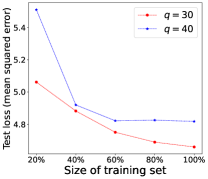
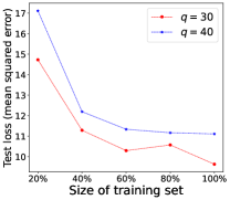
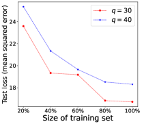
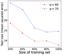
Performance of Increasing Training Data. We demonstrate in Theorem 4.4 that the model learned by our proposed LM can converge to the optimal model learned from the fully labeled data when the number of training examples for RIT approaches infinity. To empirically validate such a theoretical finding, we further conduct experiments by changing the fraction of training examples for RIT, where 100% indicates the use of all training examples to train the model. The experimental performance of LM is shown in Figure 2, where the test loss of the model generally decreases when more training examples are used to train the model. This empirical observation accords with our theoretical analysis that the learned model will be closer to the optimal model, if more training examples are provided.

More experimental results. We provide more experimental results including the comparison results with the fully supervised method, maximum margin interval trees method (MMIT (Drouin et al., 2017)), and more results on evaluation metrics and models in Appendix F. These results also demonstrate the effectiveness of our method.

6 Conclusion

In this paper, we studied an interesting weakly supervised regression setting called regression with interval targets (RIT). For the RIT setting, we first proposed a novel statistical model to describe the data generation process for RIT and demonstrated its validity. The explicitly derived data distribution can be helpful to empirical risk minimization. Then, we analyzed a simple selection method that selects a particular value in the interval as the target value to train the model. We empirically showed that this simple method could work well if the middlemost value in the interval is selected. Afterward, we proposed a statistically consistent limiting method to train the model by limiting the predictions to the interval. We further derived an estimation error bound for this method. Finally, we conducted extensive experiments on various datasets to demonstrate the effectiveness of our proposed method. In future work, it would be interesting to study a harder setting of RIT, where the true target value might be outside the given interval.

Acknowledgements

This research is supported, in part, by the Joint NTU-WeBank Research Centre on Fintech (Award No: NWJ-2021-005), Nanyang Technological University, Singapore. Lei Feng is also supported by the National Natural Science Foundation of China (Grant No. 62106028), Chongqing Overseas Chinese Entrepreneurship and Innovation Support Program, CAAI-Huawei MindSpore Open Fund, and Chongqing Artificial Intelligence Innovation Center. Ximing Li is supported by the National Key R&D Program of China (No. 2021ZD0112501, No. 2021ZD0112502) and the National Natural Science Foundation of China (No. 62276113).

References

Amar et al. (2001) Amar, R. A., Dooly, D. R., Goldman, S. A., and Zhang, Q. Multiple-instance learning of real-valued data. In ICML, pp. 3–10, 2001.
Billard (2006) Billard, L. Symbolic data analysis: what is it? In Compstat 2006-Proceedings in Computational Statistics: 17th Symposium Held in Rome, Italy, 2006, pp. 261–269. Springer, 2006.
Billard & Diday (2000) Billard, L. and Diday, E. Regression analysis for interval-valued data. In Data Analysis, Classification, and Related Methods, pp. 369–374. Springer, 2000.
Bock & Diday (1999) Bock, H.-H. and Diday, E. Analysis of symbolic data: exploratory methods for extracting statistical information from complex data. Springer Science & Business Media, 1999.
Carpentier & Schlüter (2016) Carpentier, A. and Schlüter, T. Learning relationships between data obtained independently. In AISTATS, pp. 658–666, 2016.
Cer et al. (2017) Cer, D., Diab, M., Agirre, E., Lopez-Gazpio, I., and Specia, L. Semeval-2017 task 1: Semantic textual similarity-multilingual and cross-lingual focused evaluation. arXiv preprint arXiv:1708.00055, 2017.
Cour et al. (2011) Cour, T., Sapp, B., and Taskar, B. Learning from partial labels. The Journal of Machine Learning Research, 12:1501–1536, 2011.
Drouin et al. (2017) Drouin, A., Hocking, T., and Laviolette, F. Maximum margin interval trees. In NeurIPS, 2017.
Dua & Graff (2017) Dua, D. and Graff, C. UCI machine learning repository, 2017. URL http://archive.ics.uci.edu/ml.
Fagundes et al. (2014) Fagundes, R. A., De Souza, R. M., and Cysneiros, F. J. A. Interval kernel regression. Neurocomputing, 128:371–388, 2014.
Feng et al. (2020) Feng, L., Lv, J., Han, B., Xu, M., Niu, G., Geng, X., An, B., and Sugiyama, M. Provably consistent partial-label learning. In NeurIPS, pp. 10948–10960, 2020.
Geng et al. (2013) Geng, X., Yin, C., and Zhou, Z.-H. Facial age estimation by learning from label distributions. IEEE Transactions on Pattern Analysis and Machine Intelligence, 35(10):2401–2412, 2013.
Giordani (2015) Giordani, P. Lasso-constrained regression analysis for interval-valued data. Advances in Data Analysis and Classification, 9(1):5–19, 2015.
He et al. (2016) He, K., Zhang, X., Ren, S., and Sun, J. Deep residual learning for image recognition. In CVPR, pp. 770–778, 2016.
Hu et al. (2020) Hu, W., Li, Z., and Yu, D. Simple and effective regularization methods for training on noisily labeled data with generalization guarantee. In ICLR, 2020.
Ishibuchi & Tanaka (1991) Ishibuchi, H. and Tanaka, H. An extension of the bp-algorithm to interval input vectors-learning from numerical data and expert’s knowledge. In IJCNN, pp. 1588–1593, 1991.
Ishida et al. (2019) Ishida, T., Niu, G., Menon, A., and Sugiyama, M. Complementary-label learning for arbitrary losses and models. In ICML, pp. 2971–2980, 2019.
Kingma & Ba (2015) Kingma, D. P. and Ba, J. Adam: A method for stochastic optimization. In ICLR, 2015.
Kleinbaum et al. (2012) Kleinbaum, D. G., Klein, M., et al. Survival analysis: a self-learning text, volume 3. Springer, 2012.
Kostopoulos et al. (2018) Kostopoulos, G., Karlos, S., Kotsiantis, S., and Ragos, O. Semi-supervised regression: A recent review. Journal of Intelligent & Fuzzy Systems, 35(2):1483–1500, 2018.
Lauro & Palumbo (2000) Lauro, C. N. and Palumbo, F. Principal component analysis of interval data: a symbolic data analysis approach. Computational Statistics, 15(1):73–87, 2000.
Lesaffre et al. (2005) Lesaffre, E., Komárek, A., and Declerck, D. An overview of methods for interval-censored data with an emphasis on applications in dentistry. Statistical Methods in Medical Research, 14(6):539–552, 2005.
Li et al. (2017) Li, Y.-F., Zha, H.-W., and Zhou, Z.-H. Learning safe prediction for semi-supervised regression. In AAAI, 2017.
Lindsey & Ryan (1998) Lindsey, J. C. and Ryan, L. M. Methods for interval-censored data. Statistics in Medicine, 17(2):219–238, 1998.
Lv et al. (2020) Lv, J., Xu, M., Feng, L., Niu, G., Geng, X., and Sugiyama, M. Progressive identification of true labels for partial-label learning. In ICML, 2020.
Machin et al. (2006) Machin, D., Cheung, Y. B., and Parmar, M. Survival analysis: a practical approach. John Wiley & Sons, 2006.
Manski & Tamer (2002) Manski, C. F. and Tamer, E. Inference on regressions with interval data on a regressor or outcome. Econometrica, 70(2):519–546, 2002.
Mohri et al. (2012) Mohri, M., Rostamizadeh, A., and Talwalkar, A. Foundations of Machine Learning. MIT Press, 2012.
Moschoglou et al. (2017) Moschoglou, S., Papaioannou, A., Sagonas, C., Deng, J., Kotsia, I., and Zafeiriou, S. Agedb: The first manually collected, in-the-wild age database. In CVPRW, pp. 1997–2005, 2017.
Neto & De Carvalho (2008) Neto, E. d. A. L. and De Carvalho, F. D. A. Centre and range method for fitting a linear regression model to symbolic interval data. Computational Statistics & Data Analysis, 52(3):1500–1515, 2008.
Neto & De Carvalho (2010) Neto, E. d. A. L. and De Carvalho, F. D. A. Constrained linear regression models for symbolic interval-valued variables. Computational Statistics & Data Analysis, 54(2):333–347, 2010.
Park et al. (2020) Park, S., Wang, X., Lim, J., Xiao, G., Lu, T., and Wang, T. Bayesian multiple instance regression for modeling immunogenic neoantigens. Statistical Methods in Medical Research, 29(10):3032–3047, 2020.
Patrini et al. (2017) Patrini, G., Rozza, A., Krishna Menon, A., Nock, R., and Qu, L. Making deep neural networks robust to label noise: A loss correction approach. In CVPR, pp. 1944–1952, 2017.
Rabinowitz et al. (1995) Rabinowitz, D., Tsiatis, A., and Aragon, J. Regression with interval-censored data. Biometrika, 82(3):501–513, 1995.
Ristovski et al. (2010) Ristovski, K., Das, D., Ouzienko, V., Guo, Y., and Obradovic, Z. Regression learning with multiple noisy oracles. In ECAI, pp. 445–450, 2010.
Rothe et al. (2018) Rothe, R., Timofte, R., and Van Gool, L. Deep expectation of real and apparent age from a single image without facial landmarks. International Journal of Computer Vision, 126(2):144–157, 2018.
Sadeghi et al. (2019) Sadeghi, J., De Angelis, M., and Patelli, E. Efficient training of interval neural networks for imprecise training data. Neural Networks, 118:338–351, 2019.
Stulp & Sigaud (2015) Stulp, F. and Sigaud, O. Many regression algorithms, one unified model: A review. Neural Networks, 69:60–79, 2015.
Sun (2006) Sun, J. The statistical analysis of interval-censored failure time data. Springer, 2006.
Uysal & Güvenir (1999) Uysal, I. and Güvenir, H. A. An overview of regression techniques for knowledge discovery. The Knowledge Engineering Review, 14(4):319–340, 1999.
Wang et al. (2019a) Wang, A., Singh, A., Michael, J., Hill, F., Levy, O., and Bowman, S. R. Glue: A multi-task benchmark and analysis platform for natural language understanding. In ICLR, 2019a.
Wang et al. (2019b) Wang, P., Li, Y., and Reddy, C. K. Machine learning for survival analysis: A survey. ACM Computing Surveys, 51(6):1–36, 2019b.
Wang et al. (2011) Wang, Z., Lan, L., and Vucetic, S. Mixture model for multiple instance regression and applications in remote sensing. IEEE Transactions on Geoscience and Remote Sensing, 50(6):2226–2237, 2011.
Wasserman & Lafferty (2007) Wasserman, L. and Lafferty, J. Statistical analysis of semi-supervised regression. In NeurIPS, 2007.
Xu et al. (2019) Xu, L., Honda, J., Niu, G., and Sugiyama, M. Uncoupled regression from pairwise comparison data. In NeurIPS, 2019.
Yang & Liu (2018) Yang, D. and Liu, Y. L1/2 regularization learning for smoothing interval neural networks: Algorithms and convergence analysis. Neurocomputing, 272:122–129, 2018.
Yang & Wu (2012) Yang, D. and Wu, W. A smoothing interval neural network. Discrete Dynamics in Nature and Society, 2012, 2012.
Yang et al. (2021) Yang, Y., Zha, K., Chen, Y., Wang, H., and Katabi, D. Delving into deep imbalanced regression. In ICML, pp. 11842–11851, 2021.
Yang et al. (2019) Yang, Z., Lin, D. K., and Zhang, A. Interval-valued data prediction via regularized artificial neural network. Neurocomputing, 331:336–345, 2019.

Appendix A Proofs about the Problem Setting

A.1 Prove of Theorem 3.1

For a specific label $y$ , we define the set of all the possible intervals whose size is less than $q$ as

\mathcal{S}_{q}^{y}=\{S\mid S\in\mathcal{S},|S|\leq q,y\in S\}

Since $\mathcal{S}_{q}^{y}$ is a continuous space, we use the sum of the number of all possible intervals to represent the size of $\mathcal{S}_{q}^{y}$ , that is, the integral over all possible intervals. We might as well discuss the range of values of $\underline{y}$ and then fix $\underline{y}$ to discuss the values of $\overline{y}$ . We can easily know that $\underline{y}\in[y-q,y]$ . If $\underline{y}<y-q$ , even the largest interval $S^{\prime}=[\underline{y},\underline{y}+q]$ cannot contain $y$ ( $\underline{y}+q<y$ ). If $\underline{y}>y$ , then the interval must not contain $y$ ( $\underline{y}>y$ ). After determining $\underline{y}$ , the maximum value of $\overline{y}$ is $\underline{y}+q$ ( $\overline{y}-\underline{y}\leq q$ ) and the minimum value is $y$ ( $y\leq\overline{y}$ ), so $\overline{y}\in[y,\underline{y}+q]$ , then $|\mathcal{S}_{q}^{y}|=\int_{y-q}^{y}\int_{y}^{\underline{y}+q}1\ \mathrm{d}\overline{y}\mathrm{d}\underline{y}=\frac{q^{2}}{2}$ . From our formulation of the interval data distribution $\tilde{p}(\bm{x},S)$ , we can obtain the simplified expression $\tilde{p}(\bm{x},S)=\frac{2}{q^{2}}\int_{y\in S}p(\bm{x},y)\ \mathrm{d}y$ . Then, we have

	$\displaystyle\int_{\mathcal{S}}\int_{\mathcal{X}}\tilde{p}(\bm{x},S)\mathrm{d}\bm{x}\ \mathrm{d}S$	$\displaystyle=\int_{\mathcal{X}}\int_{\mathcal{S}}\int_{y\in\mathcal{S}}\frac{2}{q^{2}}p(\bm{x},y)\ \mathrm{d}y\mathrm{d}S\mathrm{d}\bm{x}$
		$\displaystyle=\frac{2}{q^{2}}\int_{\mathcal{X}}\int_{\mathcal{Y}}\int_{\mathcal{S}_{q}^{y}}p(\bm{x},y)\ \mathrm{d}S\mathrm{d}y\mathrm{d}\bm{x}$
		$\displaystyle=\frac{2}{q^{2}}\int_{\mathcal{X}}\int_{\mathcal{Y}}p(\bm{x},y)\int_{\mathcal{S}_{q}^{y}}1\ \mathrm{d}S\mathrm{d}y\mathrm{d}\bm{x}$
		$\displaystyle=\frac{2}{q^{2}}\int_{\mathcal{X}}\int_{\mathcal{Y}}p(\bm{x},y)\|\mathcal{S}_{q}^{y}\|\mathrm{d}y\mathrm{d}\bm{x}$
		$\displaystyle=\frac{2}{q^{2}}\int_{\mathcal{X}}\int_{\mathcal{Y}}p(\bm{x},y)\frac{q^{2}}{2}\mathrm{d}y\mathrm{d}\bm{x}$
		$\displaystyle=\int_{\mathcal{X}}\int_{\mathcal{Y}}p(\bm{x},y)\mathrm{d}y\mathrm{d}\bm{x}$
		$\displaystyle=1,$

which concludes the proof of Theorem 3.1.∎

A.2 Prove of Theorem 3.2

It is intuitive to express $\mathrm{Pr}[y\in S|\bm{x},S]$ as

	$\displaystyle\mathrm{Pr}[y\in S\|\bm{x},S]$	$\displaystyle=1-\mathrm{Pr}[y\notin S\|\bm{x},S]$
		$\displaystyle=1-\int_{y\notin S}p(y\|\bm{x},S)\mathrm{d}y$
		$\displaystyle=1-\int_{y\notin S}\frac{p(S\|y,\bm{x})p(y,\bm{x})}{p(S\|\bm{x})}\mathrm{d}y$
		$\displaystyle=1-\int_{y\notin S}\frac{p(S\|y)p(y,\bm{x})}{\int_{y^{\prime}\in S}p(S\|y^{\prime})p(y^{\prime}\|\bm{x})\mathrm{d}y^{\prime}}\mathrm{d}y$
		$\displaystyle=1-\|\mathcal{S}_{q}^{y^{\prime}}\|\int_{y\notin S}\frac{p(S\|y)p(y,\bm{x})}{\int_{y\in S}p(y^{\prime}\|\bm{x})\mathrm{d}y^{\prime}}\mathrm{d}y$
		$\displaystyle=1-\frac{q^{2}}{2}\int_{y\notin S}\frac{p(S\|y)p(y,\bm{x})}{\int_{y^{\prime}\in S}p(y^{\prime}\|\bm{x})\mathrm{d}y^{\prime}}\mathrm{d}y$
		$\displaystyle=1,$

where the last equality holds because $p(S|y)=0$ if $y\notin S$ , in terms of Eq. (3). Which concludes the proof of Theorem 3.2.∎

A.3 Prove of Lemma 3.3

We consider the case where the true label $y$ is a specific value, then we have

	$\displaystyle p(y\in S,y\|\bm{x})$	$\displaystyle=\mathrm{Pr}[y\in S\|\bm{x},y]p(y\|\bm{x})$
		$\displaystyle=\int_{\mathcal{S}}p(y\in S,S\|\bm{x},y)p(y\|\bm{x})\ \mathrm{d}S$
		$\displaystyle=\int_{\mathcal{S}}\mathrm{Pr}[y\in S\|\bm{x},y,S]p(y\|\bm{x})p(S\|\bm{x},y)\ \mathrm{d}S$
		$\displaystyle=\int_{\mathcal{S}}\mathrm{Pr}[y\in S\|\bm{x},y,S]p(y\|\bm{x})p(S)\ \mathrm{d}S$

where the last equality holds due to the fact that for each example $(\bm{x},y)$ , $S$ is uniformly and randomly chosen, if $q$ is specific, $p(S)=\frac{1}{|\mathcal{S}_{q}|}$ . As with $\mathcal{S}_{q}^{y}$ , we integrate over all possible intervals to calculate the size of $|\mathcal{S}_{q}|$ . We can easily know that when $\underline{y}\in[y_{\mathrm{min}}-q,y_{\mathrm{min}}]$ , $\overline{y}\in[y_{\mathrm{min}},\underline{y}+q]$ , when $\underline{y}\in[y_{\mathrm{min}},y_{\mathrm{max}}]$ , $\overline{y}\in[\underline{y},\underline{y}+q]$ , so $|S_{q}|=\int_{y_{\mathrm{min}}-q}^{y_{\mathrm{min}}}\int_{y_{\mathrm{min}}}^{\underline{y}+q}1\ \mathrm{d}y_{r}\mathrm{d}\underline{y}+\int_{y_{\mathrm{min}}}^{y_{\mathrm{max}}}\int_{\underline{y}}^{\underline{y}+q}1\ \mathrm{d}\overline{y}\mathrm{d}\underline{y}=\frac{1}{2}q^{2}+q(y_{\mathrm{max}}-y_{\mathrm{min}})$ , we have

	$\displaystyle p(y\in S,y\|\bm{x})$	$\displaystyle=\int_{\mathcal{S}}\mathrm{Pr}[y\in S\|\bm{x},y,S]p(y\|\bm{x})p(S)\ \mathrm{d}S$
		$\displaystyle=\frac{2}{2q(y_{\mathrm{max}}-y_{\mathrm{min}})+q^{2}}\int_{\mathcal{S}}\mathrm{Pr}[y\in S\|\bm{x},y,S]p(y\|\bm{x})\ \mathrm{d}S$
		$\displaystyle=\frac{2}{2q(y_{\mathrm{max}}-y_{\mathrm{min}})+q^{2}}\int_{\mathcal{S}}\mathrm{Pr}[y\in S\|\bm{x},y,S]\mathrm{d}S\ p(y\|\bm{x})$
		$\displaystyle=\frac{2}{2q(y_{\mathrm{max}}-y_{\mathrm{min}})+q^{2}}\|\mathcal{S}_{q}^{y}\|p(y\|\bm{x})$
		$\displaystyle=\frac{2}{2q(y_{\mathrm{max}}-y_{\mathrm{min}})+q^{2}}\frac{q^{2}}{2}p(y\|\bm{x})\quad(\because\|\mathcal{S}_{q}^{y}\|=\frac{q^{2}}{2})$
		$\displaystyle=\frac{q}{2(y_{\mathrm{max}}-y_{\mathrm{min}})+q}p(y\|\bm{x})$

By integrating $y$ on both sides, we can obtain

\displaystyle\mathrm{Pr}[y\in S|\bm{x}]=\frac{q}{2(y_{\mathrm{max}}-y_{\mathrm{min}})+q}

which concludes the proof of Lemma 3.3.∎

A.4 Prove of Theorem 3.4

Let us express $p(S|y\in S,\bm{x})$ as

	$\displaystyle p(S\|y\in S,\bm{x})$	$\displaystyle=\frac{p(y\in S,S\|\bm{x})}{\mathrm{Pr}[y\in S\|\bm{x}]}$
		$\displaystyle=\frac{\mathrm{Pr}[y\in S\|S,\bm{x}]p(S\|\bm{x})}{\mathrm{Pr}[y\in S\|\bm{x}]}$
		$\displaystyle=\frac{\mathrm{Pr}[y\in S\|S,\bm{x}]p(S)}{\mathrm{Pr}[y\in S\|\bm{x}]}$

where the last equality holds due to the fact that for each instance $\bm{x}$ , $S$ is uniformly and randomly chosen. Since $p(S)=\frac{1}{|S_{q}|}$ if $q$ is specific. We can easily know that when $\underline{y}\in[y_{\mathrm{min}}-q,y_{\mathrm{min}}]$ , $\overline{y}\in[y_{\mathrm{min}},\underline{y}+q]$ , when $\underline{y}\in[y_{\mathrm{min}},y_{\mathrm{max}}]$ , $\overline{y}\in[\underline{y},\underline{y}+q]$ , so $|S_{q}|=\int_{y_{\mathrm{min}}-q}^{y_{\mathrm{min}}}\int_{y_{\mathrm{min}}}^{\underline{y}+q}1\ \mathrm{d}\overline{y}\mathrm{d}\underline{y}+\int_{y_{\mathrm{min}}}^{y_{\mathrm{max}}}\int_{\underline{y}}^{\underline{y}+q}1\ \mathrm{d}\overline{y}\mathrm{d}\underline{y}=\frac{1}{2}q^{2}+q(y_{\mathrm{max}}-y_{\mathrm{min}})$ , we have

	$\displaystyle p(S\|y\in S,\bm{x})$	$\displaystyle=\frac{\mathrm{Pr}[y\in S\|S,\bm{x}]p(S)}{\mathrm{Pr}[y\in S\|\bm{x}]}$
		$\displaystyle=\frac{2}{2q(y_{\mathrm{max}}-y_{\mathrm{min}})+q^{2}}\frac{\mathrm{Pr}[y\in S\|S,\bm{x}]}{\mathrm{Pr}[y\in S\|\bm{x}]}$
		$\displaystyle=\frac{2}{2q(y_{\mathrm{max}}-y_{\mathrm{min}})+q^{2}}\frac{2(y_{\mathrm{max}}-y_{\mathrm{min}}+q)}{q}\mathrm{Pr}[y\in S\|S,\bm{x}]\quad(by\ Lemma\ \ref{lem1})$
		$\displaystyle=\frac{2}{q^{2}}\mathrm{Pr}[y\in S\|S,\bm{x}]$
		$\displaystyle=\int_{y\in S}\frac{2}{q^{2}}p(y\|\bm{x})\mathrm{d}y$

By multiplying $p(\bm{x})$ on both side, we have

	$\displaystyle p(\bm{x},S\|y\in S)$	$\displaystyle=\int_{y\in S}\frac{2}{q^{2}}p(\bm{x},y)\mathrm{d}y$
		$\displaystyle=\int_{y_{l}}^{y_{r}}\frac{2}{q^{2}}p(\bm{x},y)\mathrm{d}y$
		$\displaystyle=\tilde{p}(\bm{x},S)$

which concludes the proof of Theorem 3.4.∎

Appendix B Proofs of The Model Consistent

B.1 Prove of Theorem 4.1

First, we prove that the optimal model $f^{\star}$ learned from ordinary regression expected risk (1) is also the optimal model for $R_{LM}(f)$ as follows.

\begin{split}R_{\mathrm{LM}}(f^{\star})&=\mathbb{E}_{\tilde{p}(\bm{x},S)}[\ell_{\mathrm{LM}}(f^{\star}(\bm{x}),S)]\\ &=\int_{\mathcal{X}}\int_{\mathcal{S}}\tilde{p}(\bm{x},S)\ell_{\mathrm{LM}}(f^{\star}(\bm{x}),S)\mathrm{d}S\mathrm{d}\bm{x}\\ &=\int_{\mathcal{X}}\int_{\mathcal{S}}\int_{\mathcal{Y}}p(\bm{x},y,S)\ell_{\mathrm{LM}}(f^{\star}(\bm{x}),S)\mathrm{d}y\mathrm{d}S\mathrm{d}\bm{x}\\ &=\int_{\mathcal{X}}\int_{\mathcal{S}}\int_{\mathcal{Y}}p(S|\bm{x},y)p(y|\bm{x})p(\bm{x})\ell_{\mathrm{LM}}(f^{\star}(\bm{x}),S)\mathrm{d}y\mathrm{d}S\mathrm{d}\bm{x}\\ &=\int_{\mathcal{X}}\int_{\mathcal{Y}}p(y|\bm{x})p(\bm{x})\ell(f^{\star}(\bm{x}),y)\mathrm{d}y\mathrm{d}\bm{x}\int_{\mathcal{S}}p(S|\bm{x},y)\mathrm{d}S\\ &=\int_{\mathcal{X}}\int_{\mathcal{Y}}\ell(f^{\star}(\bm{x}),y)p(\bm{x},y)\mathrm{d}y\mathrm{d}\bm{x}\\ &=R(f^{\star})=0\end{split}

(14)

where we used the equality $\ell_{\mathrm{LM}}(f^{\star}(\bm{x}),S)=\ell(f^{\star}(\bm{x}),y)$ . This because when the true label $y\in S$ , $\ell_{\mathrm{LM}}(f^{\star}(\bm{x}),S)=\mathbb{I}_{\{\underline{y}-f^{\star}(\bm{x})>0\}}+\mathbb{I}_{\{f^{\star}(\bm{x})-\overline{y}>0\}}=\ell(f^{\star}(\bm{x}),y)=0$ . Therefore $f^{\star}$ is the optimal model for $R_{\mathrm{LM}}$ .

On the other hand, we prove that $f^{\star}$ is the sole optimal model for $R_{\mathrm{LM}}$ by contradiction. Specifically, we assume that there is at least one other model $g$ that makes $R_{\mathrm{LM}}(g)=0$ and predicts a label $y_{g}\neq y$ for at least one instance $\bm{x}$ . Therefore, for any $S$ containing $y_{g}$ we have

\displaystyle\ell_{\mathrm{LM}}(g(\bm{x}),S)=\mathbb{I}_{\{\underline{y}-y_{g}>0\}}+\mathbb{I}_{\{y_{g}-\overline{y}>0\}}=0

(15)

Nevertheless, the above equality could be always true on the condition that $y_{g}$ is invariably included in the interval $S$ of $\bm{x}$ . In the problem setting, there is no other false label that always occurs with true label in the interval $S$ . Therefore, there is one, and only one minimizer of $R_{\mathrm{LM}}$ , which is the same as the minimizer $f^{\star}$ learned from fully labeled data. The proof is completed.∎

B.2 Prove of Theorem 4.2

First, we prove that the optimal model $f_{\mathrm{LM}}^{\star}$ learned from limiting method expected risk (11) is also the optimal model for $R^{\psi}_{\mathrm{LM}}(f)$ as follows.

\begin{split}R^{\psi}_{\mathrm{LM}}(f^{\star}_{\mathrm{LM}})&=\mathbb{E}_{\tilde{p}(\bm{x},S)}[\psi_{\mathrm{LM}}(f^{\star}_{\mathrm{LM}}(\bm{x}),S)]\\ &=\int_{\mathcal{X}}\int_{\mathcal{S}}\tilde{p}(\bm{x},S)\psi_{\mathrm{LM}}(f^{\star}_{\mathrm{LM}}(\bm{x}),S)\mathrm{d}S\mathrm{d}\bm{x}\\ &=\int_{\mathcal{X}}\int_{\mathcal{S}}\int_{\mathcal{Y}}p(\bm{x},y,S)\psi_{\mathrm{LM}}(f^{\star}_{\mathrm{LM}}(\bm{x}),S)\mathrm{d}y\mathrm{d}S\mathrm{d}\bm{x}\\ &=\int_{\mathcal{X}}\int_{\mathcal{S}}\int_{\mathcal{Y}}p(S|\bm{x},y)p(y|\bm{x})p(\bm{x})\psi_{\mathrm{LM}}(f^{\star}_{\mathrm{LM}}(\bm{x}),S)\mathrm{d}y\mathrm{d}S\mathrm{d}\bm{x}\\ &=\int_{\mathcal{X}}\int_{\mathcal{Y}}p(y|\bm{x})p(\bm{x})\ell_{\mathrm{LM}}(f^{\star}_{\mathrm{LM}}(\bm{x}),y)\mathrm{d}y\mathrm{d}\bm{x}\int_{\mathcal{S}}p(S|\bm{x},y)\mathrm{d}S\\ &=\int_{\mathcal{X}}\int_{\mathcal{Y}}\ell_{\mathrm{LM}}(f^{\star}_{\mathrm{LM}}(\bm{x}),y)p(\bm{x},y)\mathrm{d}y\mathrm{d}\bm{x}\\ &=R_{\mathrm{LM}}(f^{\star}_{\mathrm{LM}})=0\end{split}

(16)

where we used the equality $\psi_{\mathrm{LM}}(f^{\star}_{\mathrm{LM}}(\bm{x}),S)=\ell_{\mathrm{LM}}(f^{\star}_{\mathrm{LM}}(\bm{x}),y)$ . This because when the true label $y\in S$ , $\psi_{\mathrm{LM}}(f^{\star}_{\mathrm{LM}}(\bm{x}),S)=\max(0,\underline{y}-f^{\star}_{\mathrm{LM}}(\bm{x}))+\max(0,f^{\star}_{\mathrm{LM}}(\bm{x})-\overline{y})=\ell_{\mathrm{LM}}(f^{\star}_{\mathrm{LM}}(\bm{x}),y)=0$ . Therefore $f^{\star}_{\mathrm{LM}}$ is the optimal model for $R^{\psi}_{\mathrm{LM}}$ .

On the other hand, we prove that $f^{\star}_{\mathrm{LM}}$ is the sole optimal model for $R^{\psi}_{\mathrm{LM}}$ by contradiction. Specifically, we assume that there is at least one other model $h$ that makes $R^{\psi}_{\mathrm{LM}}(h)=0$ and predicts a label $y_{h}\neq y$ for at least one instance $\bm{x}$ . Therefore, for any $S$ containing $y_{h}$ we have

\displaystyle\psi_{\mathrm{LM}}(h(\bm{x}),S)=\mathrm{max}(0,\underline{y}-y_{h})+\mathrm{max}(0,y_{h}-\overline{y})=0

(17)

Nevertheless, the above equality could be always true on the condition that $y_{h}$ is invariably included in the interval $S$ of $\bm{x}$ . In the problem setting, there is no other false label that always occurs with true label in the interval $S$ . Therefore, there is one, and only one minimizer of $R^{\psi}_{\mathrm{LM}}$ , which is the same as the minimizer $f^{\star}_{\mathrm{LM}}$ learned from limiting method. By Theorem 4.1, $f^{\star}_{\mathrm{LM}}$ is the same as the minimizer $f^{\star}$ learned from fully labeled data. The proof is completed.∎

Appendix C Proof of Corollary 4.3

For any interval instance $(\bm{x},S)$ , We consider three possible cases of model prediction: the predicted value is on the left side of the interval ( $f(x)<\underline{y}$ ), the predicted value is on the right side of the interval ( $f(x)>\overline{y}$ ) and the predicted value is exactly inside the interval ( $\underline{y}\leq f(x)\leq\overline{y}$ ).

If the predicted value of the model lie on the left side of the interval, the losses of AVGL_MAE and the surrogate method are as follows.

	$\displaystyle\ell_{\mathrm{avgl\_mae}}(f(\bm{x}),S)$	$\displaystyle=\frac{1}{2}(\|f(\bm{x})-\underline{y}\|+\|f(\bm{x})-\overline{y})\|)=\frac{1}{2}(\underline{y}-f(\bm{x})+\overline{y}-f(\bm{x}))=\frac{\underline{y}+\overline{y}}{2}-f(\bm{x}),$
	$\displaystyle\psi_{\mathrm{LM}}(f(\bm{x}),S)$	$\displaystyle=\max(0,\underline{y}-f(\bm{x}))+\max(0,f(\bm{x})-\overline{y})=\underline{y}-f(\bm{x})+0=\underline{y}-f(\bm{x}).$

If the predicted value of the model lie on the right side of the interval, the losses of AVGL_MAE and the surrogate method are as follows.

	$\displaystyle\ell_{\mathrm{avgl\_mae}}(f(\bm{x}),S)$	$\displaystyle=\frac{1}{2}(\|f(\bm{x})-\underline{y}\|+\|f(\bm{x})-\overline{y})\|)=\frac{1}{2}(f(\bm{x})-\underline{y}+f(\bm{x})-\overline{y})=f(\bm{x})-\frac{\underline{y}+\overline{y}}{2},$
	$\displaystyle\psi_{\mathrm{LM}}(f(\bm{x}),S)$	$\displaystyle=\max(0,\underline{y}-f(\bm{x}))+\max(0,f(\bm{x})-\overline{y})=0+f(\bm{x})-\overline{y}=f(\bm{x})-\overline{y}.$

If the predicted value of the model lie in the interval, the losses of AVGL_MAE and the surrogate method are as follows.

	$\displaystyle\ell_{\mathrm{avgl\_mae}}(f(\bm{x}),S)$	$\displaystyle=\frac{1}{2}(\|f(\bm{x})-\underline{y}\|+\|f(\bm{x})-\overline{y})\|)=0$
	$\displaystyle\psi_{\mathrm{LM}}(f(\bm{x}),S)$	$\displaystyle=\max(0,\underline{y}-f(\bm{x}))+\max(0,f(\bm{x})-\overline{y})=0$

We can see that the losses of AVGL_MAE and the surrogate loss differ only in constant terms on the three possible cases. If our training model uses gradient descent, the gradients of AVGL_MAE and the surrogate method are the same on all three possible cases.∎

Appendix D Proof of Theorem 4.4

Before directly proving Theorem 4.4, we first introduce the following lemma.

Lemma D.1.

Let $\widehat{f}$ be the empirical risk minimizer (i.e., $\widehat{f}=\mathop{\arg\min}_{f\in\mathcal{F}}\widehat{R}(f)$ ) and $f^{\star}$ be the true risk minimizer (i.e., $f^{\star}=\mathop{\arg\min}_{f\in\mathcal{F}}R(f)$ ), then the following inequality holds:

\displaystyle R(\widehat{f})-R(f^{\star})\leq 2\sup_{f\in\mathcal{F}}\left|\widehat{R}(f)-R(f)\right|.

Proof.

It is intuitive to obtain

	$\displaystyle R(\widehat{f})-R(f^{\star})$	$\displaystyle\leq R(\widehat{f})-\widehat{R}(\widehat{f})+\widehat{R}(\widehat{f})-R(f^{\star})$
		$\displaystyle\leq R(\widehat{f})-\widehat{R}(\widehat{f})+R(\widehat{f})-R(f^{\star})$
		$\displaystyle\leq 2\sup_{f\in\mathcal{F}}\left\|\widehat{R}(f)-R(f)\right\|,$

which completes the proof. The same proof has been provided in Mohri et al. (2012). ∎

Recall that $R^{\psi}_{\mathrm{LM}}(f)$ is denoted by

	$\displaystyle R^{\psi}_{\mathrm{LM}}(f)$	$\displaystyle=\mathbb{E}_{p(\bm{x},\underline{y},\overline{y})}\big{[}\psi(\underline{y}-f(\bm{x}))+\psi(f(\bm{x})-\overline{y})\big{]}$
		$\displaystyle=\mathbb{E}_{p(\bm{x},\underline{y},\overline{y})}\big{[}\max(\underline{y}-f(\bm{x}),0)+\max(f(\bm{x})-\overline{y},0)\big{]}$
		$\displaystyle=\mathbb{E}_{p(\bm{x},\underline{y},\overline{y})}\big{[}\max(\underline{y}-f(\bm{x}),0)\big{]}+\mathbb{E}_{p(\bm{x},\underline{y},\overline{y})}\big{[}\max(f(\bm{x})-\overline{y},0)\big{]}$
		$\displaystyle=R^{\psi,l}_{\mathrm{LM}}(f)+R^{\psi,r}_{\mathrm{LM}}(f),$

where we have introduced $R^{\psi,l}_{\mathrm{LM}}(f)=\mathbb{E}_{p(\bm{x},\underline{y},\overline{y})}\big{[}\max(\underline{y}-f(\bm{x}),0)\big{]}$ and $R^{\psi,r}_{\mathrm{LM}}(f)=\mathbb{E}_{p(\bm{x},\underline{y},\overline{y})}\big{[}\max(f(\bm{x})-\overline{y},0)\big{]}$ in the last equality. In this way, we have

	$\displaystyle R^{\psi}_{\mathrm{LM}}(\widehat{f}_{\mathrm{LM}})-R^{\psi}_{\mathrm{LM}}(f^{\star})$	$\displaystyle=R^{\psi}_{\mathrm{LM}}(\widehat{f}_{\mathrm{LM}})-R^{\psi}_{\mathrm{LM}}(f^{\star}_{\mathrm{LM}})$
		$\displaystyle\leq 2\sup_{f\in\mathcal{F}}\left\|R^{\psi}_{\mathrm{LM}}(\widehat{f}_{\mathrm{LM}})-R^{\psi}_{\mathrm{LM}}(f^{\star}_{\mathrm{LM}})\right\|$
		$\displaystyle\leq 2\sup_{f\in\mathcal{F}}\left\|R^{\psi,l}_{\mathrm{LM}}(\widehat{f}_{\mathrm{LM}})-R^{\psi,l}_{\mathrm{LM}}(f^{\star}_{\mathrm{LM}})\right\|+2\sup_{f\in\mathcal{F}}\left\|R^{\psi,r}_{\mathrm{LM}}(\widehat{f}_{\mathrm{LM}})-R^{\psi,r}_{\mathrm{LM}}(f^{\star}_{\mathrm{LM}})\right\|$

where the first equality holds, and the last inequality means that we can directly bound $\sup_{f\in\mathcal{F}}\left|R^{\psi,l}_{\mathrm{LM}}(\widehat{f}_{\mathrm{LM}})-R^{\psi,l}_{\mathrm{LM}}(f^{\star}_{\mathrm{LM}})\right|$ and $\sup_{f\in\mathcal{F}}\left|R^{\psi,r}_{\mathrm{LM}}(\widehat{f}_{\mathrm{LM}})-R^{\psi,r}_{\mathrm{LM}}(f^{\star}_{\mathrm{LM}})\right|$ . Based on the assumptions introduced in Theorem 4.4 and using the discussion of Theorem 10.6 in Mohri et al. (2012), with probability $1-\delta$ ,

	$\displaystyle\sup_{f\in\mathcal{F}}\left\|R^{\psi,l}_{\mathrm{LM}}(\widehat{f}_{\mathrm{LM}})-R^{\psi,l}_{\mathrm{LM}}(f^{\star}_{\mathrm{LM}})\right\|$	$\displaystyle\leq M\sqrt{\frac{2d\log\frac{en}{d}}{n}}+M\sqrt{\frac{\log\frac{2}{\delta}}{2n}},$
	$\displaystyle\sup_{f\in\mathcal{F}}\left\|R^{\psi,r}_{\mathrm{LM}}(\widehat{f}_{\mathrm{LM}})-R^{\psi,r}_{\mathrm{LM}}(f^{\star}_{\mathrm{LM}})\right\|$	$\displaystyle\leq M^{\prime}\sqrt{\frac{2d^{\prime}\log\frac{en}{d^{\prime}}}{n}}+M^{\prime}\sqrt{\frac{\log\frac{2}{\delta}}{2n}}.$

Therefore, with probability $1-\delta$ ,

\displaystyle R^{\psi}_{\mathrm{LM}}(\widehat{f}_{\mathrm{LM}})-R^{\psi}_{\mathrm{LM}}(f^{\star})\leq 2M\sqrt{\frac{2d\log\frac{en}{d}}{n}}+2M^{\prime}\sqrt{\frac{2d^{\prime}\log\frac{en}{d^{\prime}}}{n}}+2(M+M^{\prime})\sqrt{\frac{\log\frac{4}{\delta}}{2n}},

which completes the proof of Theorem 4.4.

Appendix E Additional Information of Experiments

E.1 Details of Datasets

In our experiments, we used AgeDB, IMDB-WIKI, STS-B and 6 UCI benchmark datasets including Abalone, Airfoil, Auto-mpg, Housing, Concrete and Power-plant. For each dataset, we follow the data distribution proposed in Section 3.1 to generate interval data. Then we randomly split each dataset into training, validation, and test sets by the proportions of 60%, 20%, and 20%, respectively. Here, we provide the detailed information of these datasets we used in our experiments.

AgeDB is a regression dataset on age prediction collected by (Moschoglou et al., 2017). It contains 16.4K face images with a minimum age of 0 and a maximum age of 101. We generated the interval regression dataset AgeDB-Interval at $q$ = 10, 20, 30, 40, and 50, respectively, and manually corrected the unreasonable intervals, such as intervals containing negative ages and intervals containing too old ages (less than 0 and greater than 150).

IMDB-WIKI is a regression dataset about age prediction collected by (Rothe et al., 2018). It contains 523.0K face images, and we filtered the images that do not match the criteria and finally kept 213.5K images, where the minimum age is 0 years and the maximum age is 186 years. We generated the interval regression dataset IMDB-WIKI-Interval at $q$ = 20, 30, and 40, respectively, and manually corrected the unreasonable intervals, such as those containing negative ages and those containing too old ages (less than 0 and greater than 200).

Semantic Textual Similarity Benchmark (STS-B) (Cer et al., 2017) is a collection of sentence pairs extracted from news headlines, video and image captions, and natural language inference data. Each sentence pair is scored for similarity by multiple annotators, and the final score is averaged as the final score. We created a dataset with 15.7K from (Yang et al., 2021). We generated interval regression datasets for STS-B-Interval at $q$ = 3.0, 3.5, 4.0, 4.5 and 5.0, respectively.

We conducted experiments on 6 UCI benchmark datasets including Abalone, Airfoil, Auto-mpg, Housing, Concrete and Power-plant. All of these datasets can be downloaded from the UCI Machine Learning. Based on the span of the dataset labels, we selected two larger q values to generate interval regression data for each dataset.

E.2 Evaluation Metrics

We describe in detail all the evaluation metrics we used in our experiments.

MSE. The mean squared error (MSE) is defined as $\frac{1}{n}\sum_{i=1}^{n}(y_{i}-\widehat{y}_{i})^{2}$ , where $n$ denotes the number of samples, $y_{i}$ denotes the ground truth value, and $\widehat{y}_{i}$ denotes the predicted value. MSE represents the averaged squared difference between the ground truth and predicted values over all samples.

MAE. The mean absolute error (MAE) is defined as $\frac{1}{n}\sum_{i=1}^{n}|y_{i}-\widehat{y}_{i}|$ , where $n$ denotes the number of samples, $y_{i}$ denotes the ground truth value, and $\widehat{y}_{i}$ denotes the predicted value. MAE represents the averaged absolute difference between the ground truth and predicted values over all samples.

GM. We use the Geometric Mean (GM) proposed by (Yang et al., 2021) as our evaluation method, and is defined as $(\prod\nolimits_{i=1}^{n}e_{i})^{\frac{1}{n}}$ , where $e_{i}\triangleq|y_{i}-\widehat{y}_{i}|$ . GM is using the geometric mean to describe the fairness of the model predictions rather than the arithmetic mean.

Pearson correlation. Pearson correlation is an evaluation of the linear relationship between the predicted value and the ground truth value, and is defined as $\frac{\sum_{i=1}^{n}(y_{i}-\overline{y})(\widehat{y}_{i}-\overline{\widehat{y}})}{\sqrt{\sum_{i=1}^{n}(y_{i}-\overline{y})^{2}}\sqrt{\sum_{i=1}^{n}(\widehat{y}_{i}-\overline{\widehat{y}})^{2}}}$ , where $\overline{y}$ denotes the average of all ground truth values, $\overline{\widehat{y}}$ denotes the average of all predicted values, i.e., $\overline{y}=\frac{1}{n}\sum_{i=1}^{n}y_{i}$ , $\overline{\widehat{y}}=\frac{1}{n}\sum_{i=1}^{n}\widehat{y}_{i}$ .

Table 5: Complete evaluation results on AgeDB

Metric		MSE					MAE					GM
Approach		$q=30$	$q=40$	$q=50$	$q=60$	$q=70$	$q=30$	$q=40$	$q=50$	$q=60$	$q=70$	$q=30$	$q=40$	$q=50$	$q=60$	$q=70$
Supervised		102.71					7.82					5.22
Supervised		(3.12)					(0.14)					(0.13)
LEFT	MAE	158.38	210.34	205.75	283.83	355.59	9.88	11.59	11.27	13.62	14.93	6.32	7.69	7.37	9.14	10.00
	MAE	(6.71)	(19.85)	(22.04)	(15.36)	(105.16)	(0.22)	(0.61)	(0.80)	(0.62)	(2.38)	(0.13)	(0.32)	(0.67)	(0.40)	(1.77)
	MSE	134.99	196.83	221.54	295.49	347.27	9.25	11.19	11.91	13.90	14.98	6.08	7.46	7.88	9.54	10.47
	MSE	(4.03)	(19.28)	(18.04)	(32.09)	(80.77)	(0.06)	(0.71)	(0.48)	(1.24)	(2.10)	(0.04)	(0.55)	(0.39)	(1.18)	(1.83)
	Huber	156.34	175.95	208.03	317.17	360.11	9.85	10.54	11.42	14.39	15.41	6.37	7.00	7.56	9.62	10.64
	Huber	(17.95)	(7.61)	(18.36)	(22.57)	(53.12)	(0.57)	(0.19)	(0.61)	(0.37)	(1.30)	(0.33)	(0.14)	(0.59)	(0.05)	(1.16)
RIGHT	MAE	154.87	196.95	233.18	255.24	428.05	9.91	11.31	12.48	13.12	17.51	6.64	7.74	8.67	8.97	12.77
	MAE	(13.12)	(20.96)	(26.58)	(15.12)	(41.79)	(0.45)	(0.58)	(0.79)	(0.40)	(0.93)	(0.39)	(0.40)	(0.65)	(0.29)	(0.94)
	MSE	146.85	215.06	260.37	304.71	452.61	9.57	11.96	13.27	14.47	18.15	6.34	8.04	9.12	10.28	13.31
	MSE	(24.39)	(23.92)	(15.32)	(49.88)	(45.87)	(0.86)	(0.66)	(0.49)	(1.29)	(1.15)	(0.87)	(0.54)	(0.34)	(1.10)	(1.26)
	Huber	149.14	179.72	246.29	279.70	436.29	9.72	10.84	12.88	13.90	17.50	6.54	7.41	8.85	9.77	12.77
	Huber	(7.74)	(10.57)	(16.02)	(17.45)	(78.90)	(0.31)	(0.37)	(0.48)	(0.44)	(1.86)	(0.19)	(0.25)	(0.63)	(0.24)	(1.79)
Middle	MAE	116.14	133.44	129.55	138.95	150.88	8.38	8.93	8.97	9.21	9.57	5.44	5.75	6.22	5.93	6.35
	MAE	(2.57)	(5.05)	(1.37)	(5.22)	(3.66)	(0.13)	(0.15)	(0.13)	(0.11)	(0.12)	(0.04)	(0.04)	(0.72)	(0.08)	(0.11)
	MSE	119.90	133.27	128.84	138.36	149.82	8.45	8.94	8.89	9.32	9.53	5.57	5.91	5.75	6.16	6.33
	MSE	(6.23)	(5.18)	(3.01)	(6.10)	(5.28)	(0.18)	(0.22)	(0.21)	(0.27)	(0.07)	(0.18)	(0.05)	(0.10)	(0.24)	(0.03)
	Huber	121.78	131.43	131.38	140.40	149.25	8.62	8.92	8.96	9.28	9.65	5.54	5.76	5.83	6.15	6.35
	Huber	(4.75)	(3.84)	(2.20)	(6.18)	(0.70)	(0.14)	(0.15)	(0.08)	(0.19)	(0.09)	(0.07)	(0.10)	(0.05)	(0.18)	(0.12)
CRM		221.66	303.52	398.50	523.53	653.81	12.18	14.57	17.17	20.11	22.89	8.42	10.51	12.82	15.86	18.63
CRM		(1.45)	(11.12)	(14.80)	(4.63)	(17.30)	(0.07)	(0.30)	(0.40)	(0.08)	(0.09)	(0.07)	(0.24)	(0.44)	(0.20)	(0.21)
RANN		125.04	126.02	129.86	139.83	148.25	8.69	8.73	8.89	9.32	9.69	5.62	5.69	5.92	6.82	6.42
RANN		(1.09)	(1.74)	(1.00)	(3.41)	(2.33)	(0.04)	(0.07)	(0.05)	(0.22)	(0.11)	(0.12)	(0.07)	(0.03)	(1.01)	(0.09)
SINN		218.16	302.06	404.80	524.74	649.27	12.11	14.54	17.41	19.97	22.70	8.39	10.45	13.32	15.69	18.52
SINN		(1.53)	(6.53)	(2.70)	(7.17)	(2.94)	(0.08)	(0.24)	(0.04)	(0.13)	(0.14)	(0.14)	(0.29)	(0.13)	(0.24)	(0.25)
IN		118.85	133.86	138.58	147.95	152.34	8.46	9.00	9.15	9.53	9.65	5.75	5.88	5.94	6.23	6.30
IN		(5.20)	(6.46)	(4.06)	(2.82)	(9.30)	(0.17)	(0.13)	(0.09)	(0.07)	(0.21)	(0.25)	(0.09)	(0.05)	(0.16)	(0.15)
LM		115.76	121.24	123.51	128.04	129.47	8.36	8.67	8.75	8.82	8.92	5.41	5.61	5.65	5.73	5.84
LM		(1.64)	(4.73)	(2.78)	(3.52)	(7.15)	(0.07)	(0.03)	(0.14)	(0.16)	(0.14)	(0.03)	(0.02)	(0.13)	(0.07)	(0.11)

Table 6: All results on IMDB-WIKI.

Metrics		MSE					MAE					GM
Approach		$q=40$	$q=50$	$q=60$	$q=70$	$q=80$	$q=40$	$q=50$	$q=60$	$q=70$	$q=80$	$q=40$	$q=50$	$q=60$	$q=70$	$q=80$
Supervised		123.82					8.38					5.40
Supervised		(3.06)					(0.07)					(0.09)
LEFT	MAE	270.15	336.73	402.05	494.84	581.54	13.06	14.76	16.28	18.30	20.39	8.60	10.09	13.54	12.98	15.28
	MAE	(15.14)	(30.92)	(39.13)	(28.64)	(19.81)	(0.53)	(0.77)	(1.10)	(0.82)	(0.46)	(0.63)	(0.53)	(2.46)	(0.93)	(0.69)
	MSE	255.40	305.92	358.15	383.77	421.16	12.67	13.95	15.21	15.86	16.66	8.24	9.35	10.34	10.91	11.70
	MSE	(13.45)	(7.33)	(25.61)	(16.82)	(94.72)	(0.40)	(0.60)	(0.57)	(0.36)	(2.36)	(0.43)	(0.29)	(0.42)	(0.45)	(2.36)
	Huber	291.25	320.37	385.99	512.73	596.39	13.39	14.24	15.82	18.57	20.71	8.71	11.40	10.83	13.46	15.57
	Huber	(14.98)	(10.01)	(41.84)	(107.26)	(46.08)	(0.26)	(0.42)	(1.14)	(2.54)	(0.79)	(0.17)	(3.00)	(1.07)	(2.67)	(0.47)
RIGHT	MAE	197.26	265.60	328.77	608.51	679.26	11.15	13.38	14.74	20.80	22.82	8.07	10.74	13.29	15.69	17.55
	MAE	(17.24)	(27.79)	(63.99)	(76.85)	(80.82)	(0.62)	(0.75)	(1.55)	(1.50)	(2.21)	(0.55)	(1.61)	(3.84)	(1.31)	(3.04)
	MSE	214.42	280.99	357.06	497.47	643.99	11.71	13.50	15.29	18.82	21.38	7.82	9.17	10.48	13.63	15.55
	MSE	(10.40)	(12.52)	(64.59)	(43.98)	(85.80)	(0.35)	(0.35)	(1.54)	(1.05)	(1.49)	(0.31)	(0.32)	(1.18)	(0.96)	(1.24)
	Huber	198.97	243.81	379.34	536.87	491.39	11.23	12.82	16.19	19.63	18.24	8.48	10.84	14.15	14.14	12.83
	Huber	(6.47)	(11.64)	(45.10)	(21.50)	(103.54)	(0.21)	(0.31)	(1.01)	(0.67)	(2.22)	(0.16)	(0.16)	(2.10)	(0.48)	(1.88)
Middle	MAE	140.29	148.93	152.20	154.79	157.17	8.96	9.24	9.47	9.55	9.76	5.94	6.20	6.82	7.43	6.96
	MAE	(6.68)	(3.00)	(9.59)	(4.29)	(5.96)	(0.10)	(0.08)	(0.36)	(0.21)	(0.22)	(0.38)	(0.51)	(0.06)	(0.71)	(0.61)
	MSE	135.57	142.68	144.34	153.10	153.80	8.89	9.10	9.23	9.61	9.79	5.97	5.92	6.45	6.61	6.97
	MSE	(2.77)	(2.43)	(2.60)	(9.34)	(3.57)	(0.10)	(0.06)	(0.11)	(0.30)	(0.08)	(0.54)	(0.20)	(0.70)	(0.16)	(0.43)
	Huber	142.21	148.52	153.97	152.52	154.77	9.04	9.22	9.49	9.49	9.70	5.71	6.05	6.25	6.12	6.41
	Huber	(6.33)	(3.93)	(2.31)	(3.48)	(3.58)	(0.19)	(0.15)	(0.05)	(0.12)	(0.15)	(0.13)	(0.17)	(0.24)	(0.10)	(0.14)
CRM		302.50	380.12	519.7	602.65	740.99	14.38	16.81	20.11	21.85	24.61	10.18	12.81	13.26	18.16	21.34
CRM		(12.53)	(15.30)	(10.23)	(7.20)	(19.56)	(0.42)	(0.28)	(0.20)	(0.16)	(0.78)	(0.56)	(0.46)	(0.44)	(0.39)	(0.56)
RANN		137.37	140.79	145.40	150.11	166.33	8.98	8.98	9.32	9.52	10.09	5.82	6.14	6.74	6.85	6.63
RANN		(3.09)	(2.28)	(2.20)	(2.48)	(4.02)	(0.10)	(0.12)	(0.08)	(0.07)	(0.08)	(0.12)	(0.14)	(0.18)	(0.25	(0.10)
SINN		314.49	385.29	515.80	629.51	754.28	14.79	16.73	19.84	22.36	24.73	10.88	12.59	15.77	17.31	20.28
SINN		(4.08)	(8.26)	(9.95)	(11.10)	(15.20)	(0.14)	(0.19)	(0.30)	(0.23)	(0.65)	(0.23)	(0.45)	(0.55)	(0.72)	(0.49)
IN		147.09	148.71	152.66	155.73	156.04	9.25	9.28	9.51	9.59	9.79	6.45	7.08	6.60	6.90	7.61
IN		(0.59)	(1.01)	(2.54)	(5.67)	(2.89)	(0.04)	(0.09)	(0.10)	(0.17)	(0.06)	(0.24)	(0.36)	(0.42)	(0.70)	(0.15)
LM		133.98	134.15	141.45	148.19	146.52	8.75	8.83	9.07	9.40	9.39	5.59	5.79	5.81	6.10	6.12
LM		(1.57)	(2.49)	(2.32)	(2.44)	(5.00)	(0.06)	(0.07)	(0.11)	(0.08)	(0.04)	(0.08)	(0.20)	(0.07)	(0.10)	(0.14)

Table 7: All results on STS-B.

Metrics		MSE					MAE					Pearson
Approach		$q=3.0$	$q=3.5$	$q=4.0$	$q=4.5$	$q=5.0$	$q=3.0$	$q=3.5$	$q=4.0$	$q=4.5$	$q=5.0$	$q=3.0$	$q=3.5$	$q=4.0$	$q=4.5$	$q=5.0$
Supervised		1.16					0.87					0.71
Supervised		(0.05)					(0.02)					(0.01)
LEFT	MAE	1.54	1.88	2.35	2.63	3.03	1.01	1.11	1.26	1.33	1.43	0.69	0.66	0.64	0.62	0.59
	MAE	(0.06)	(0.06)	(0.15)	(0.13)	(0.06)	(0.02)	(0.02)	(0.05)	(0.03)	(0.02)	(0.01)	(0.01)	(0.01)	(0.02)	(0.01)
	MSE	2.02	2.16	2.55	2.88	3.13	1.17	1.20	1.32	1.40	1.47	0.66	0.65	0.63	0.61	0.58
	MSE	(0.08)	(0.07)	(0.12)	(0.11)	(0.12)	(0.03)	(0.02)	(0.03)	(0.03)	(0.04)	(0.01)	(0.01)	(0.01)	(0.01)	(0.03)
	Huber	1.92	2.26	2.51	2.76	3.05	1.14	1.23	1.31	1.37	1.44	0.67	0.65	0.63	0.61	0.59
	Huber	(0.13)	(0.10)	(0.14)	(0.10)	(0.15)	(0.04)	(0.03)	(0.05)	(0.03)	(0.04)	(0.01)	(0.01)	(0.01)	(0.01)	(0.02)
RIGHT	MAE	1.75	1.87	2.09	2.05	2.31	1.06	1.12	1.17	1.16	1.23	0.68	0.63	0.62	0.55	0.55
	MAE	(0.14)	(0.19)	(0.18)	(0.28)	(0.40)	(0.04)	(0.07)	(0.05)	(0.08)	(0.10)	(0.01)	(0.05)	(0.02)	(0.09)	(0.05)
	MSE	1.53	1.74	1.78	2.00	2.26	1.00	1.06	1.08	1.14	1.21	0.63	0.60	0.56	0.53	0.52
	MSE	(0.05)	(0.13)	(0.19)	(0.17)	(0.16)	(0.02)	(0.03)	(0.06)	(0.05)	(0.03)	(0.01)	(0.02)	(0.05)	(0.02)	(0.02)
	Huber	1.56	1.77	1.86	1.91	2.39	1.01	1.07	1.10	1.12	1.24	0.64	0.62	0.58	0.56	0.52
	Huber	(0.08)	(0.11)	(0.27)	(0.15)	(0.08)	(0.03)	(0.04)	(0.08)	(0.05)	(0.03)	(0.02)	(0.01)	(0.02)	(0.02)	(0.02)
Middle	MAE	1.18	1.23	1.27	1.31	1.41	0.88	0.91	0.92	0.94	0.98	0.69	0.66	0.66	0.64	0.62
	MAE	(0.03)	(0.05)	(0.07)	(0.03)	(0.05)	(0.01)	(0.02)	(0.03)	(0.01)	(0.02)	(0.01)	(0.02)	(0.01)	(0.01)	(0.02)
	MSE	1.31	1.33	1.41	1.41	1.49	0.94	0.95	0.98	0.99	1.02	0.65	0.64	0.62	0.61	0.59
	MSE	(0.02)	(0.05)	(0.04)	(0.01)	(0.03)	(0.01)	(0.02)	(0.01)	(0.01)	(0.01)	(0.01)	(0.02)	(0.01)	(0.01)	(0.01)
	Huber	1.37	1.30	1.37	1.39	1.48	0.96	0.94	0.97	0.97	1.01	0.64	0.64	0.62	0.62	0.59
	Huber	(0.16)	(0.04)	(0.08)	(0.02)	(0.03)	(0.06)	(0.02)	(0.03)	(0.01)	(0.01)	(0.03)	(0.01)	(0.01)	(0.01)	(0.01)
CRM		1.36	1.50	1.53	1.52	1.56	0.96	1.00	1.02	1.02	1.05	0.64	0.60	0.59	0.58	0.56
CRM		(0.02)	(0.10)	(0.08)	(0.06)	(0.06)	(0.01)	(0.04)	(0.03)	(0.02)	(0.03)	(0.01)	(0.03)	(0.03)	(0.03)	(0.02)
RANN		1.44	1.52	1.55	1.63	1.62	0.98	1.01	1.02	1.05	1.06	0.59	0.57	0.55	0.52	0.51
RANN		(0.05)	(0.04)	(0.06)	(0.06)	(0.06)	(0.02)	(0.02)	(0.03)	(0.02)	(0.03)	(0.01)	(0.02)	(0.02)	(0.02)	(0.02)
SINN		1.37	1.50	1.50	1.54	1.61	0.96	1.00	1.01	1.03	1.06	0.64	0.60	0.60	0.58	0.54
SINN		(0.04)	(0.05)	(0.10)	(0.05)	(0.09)	(0.01)	(0.01)	(0.03)	(0.02)	(0.03)	(0.01)	(0.01)	(0.02)	(0.01)	(0.03)
IN		1.26	1.39	1.37	1.37	1.41	0.91	0.96	0.96	0.96	0.98	0.67	0.62	0.62	0.62	0.61
IN		(0.12)	(0.21)	(0.14)	(0.08)	(0.07)	(0.04)	(0.06)	(0.04)	(0.03)	(0.03)	(0.04)	(0.06)	(0.05)	(0.01)	(0.01)
LM		1.19	1.22	1.27	1.31	1.37	0.88	0.90	0.93	0.94	0.96	0.69	0.66	0.65	0.64	0.62
LM		(0.04)	(0.02)	(0.04)	(0.04)	(0.05)	(0.01)	(0.01)	(0.01)	(0.01)	(0.01)	(0.01)	(0.01)	(0.01)	(0.02)	(0.02)

Appendix F Additional Results

In the experiment of main paper, we show some of the experiments on the three datasets AgeDB, IMDB-WIKI and STS-B. Here, we provide the complete evaluation results on the nine used datasets, which include more evaluation metrics in addition to the results in the main paper.

F.1 Complete Results on AgeDB

We show the complete results of AgeDB in Table 5. In the table, we show the test performance (mean and std) of each method with ResNet-50, evaluated using MSE, MAE and GM. We repeat the sampling-and-training process 3 times. The best performance is highlighted in bold. In addition, Our Vs Sup means the mean error between our proposed method and the supervised method (Our - Supervised). Specifically, we use red color to indicate that our method is weaker than the supervised method and green color to indicate that our method is better than the supervised method. As the table shows, our proposed method LM has significant advantages in all evaluation metrics.

F.2 Complete Results on IMDB-WIKI

We show the complete results of IMDB-WIKI in Table 6. Similar to AgeDB, we evaluate each method using MSE, MAE and GM. We repeat the sampling-and-training process 3 times. It is worth noting that we chose different q values for AgeDB and IMDB-WIKI, although both are age predictions. IMDB-WIKI has a larger training set, and we want to test our method on a large dataset in a harsh environment (large $q$ ). As shown in the table 6, our proposed method LM has significant advantages in all evaluation metrics. Even in the case of $q=80$ , the performance does not degrade excessively after learning from a large number of training sets.

F.3 Complete Results on STS-B

We show the complete results of STS-B in Table 7. In the table, we show the test performance (mean and std) of each method with BiLSTM + GloVe word embeddings baseline, evaluated using MSE, MAE and Pearson. Unlike AgeDB and IMDB-WIKI, STS-B has a smaller span of labels, so we can only choose smaller $q$ values to generate interval data. As shown in the table, the difference between methods is not significant when $q$ is small. As $q$ keeps increasing, all the methods tend to decrease in performance, while our method decreases more slowly and has a significant advantage at large $q$ .

Table 8: Comparison of MMIT and LM with MLP model

Metrics		MSE			MAE			Pearson			GM
Approach		Linear	Square	LM_MLP	Linear	Square	LM_MLP	Linear	Square	LM_MLP	Linear	Square	LM_MLP
Abalone	q=30	6.41	6.77	4.66	1.88	1.98	1.50	0.63	0.63	0.74	1.17	1.28	0.91
	q=30	(0.31)	(0.82)	(0.49)	(0.03)	(0.15)	(0.05)	(0.02)	(0.04)	(0.02)	(0.03)	(0.09)	(0.07)
	q=40	7.03	6.99	4.81	2.01	2.02	1.53	0.61	0.62	0.75	1.36	1.37	0.90
	q=40	(0.79)	(0.69)	(0.42)	(0.17)	(0.12)	(0.08)	(0.02)	(0.01)	(0.01)	(0.13)	(0.13)	(0.04)
Airfoil	q=30	18.74	17.98	16.72	3.33	3.25	3.09	0.80	0.80	0.81	2.15	2.03	1.93
	q=30	(3.41)	(1.70)	(3.42)	(0.30)	(0.14)	(0.35)	(0.05)	(0.04)	(0.04)	(0.22)	(0.12)	(0.27)
	q=40	23.61	19.57	18.31	3.72	3.46	3.24	0.74	0.78	0.80	2.38	2.25	2.08
	q=40	(3.20)	(1.98)	(2.63)	(0.26)	(0.16)	(0.27)	(0.03)	(0.02)	(0.03)	(0.25)	(0.16)	(0.22)
Auto-mpg	q=30	17.82	15.51	9.63	3.16	2.91	2.19	0.84	0.87	0.92	1.95	1.81	1.36
	q=30	(2.72)	(2.23)	(1.62)	(0.25)	(0.25)	(0.18)	(0.04)	(0.01)	(0.01)	(0.23)	(0.25)	(0.16)
	q=40	19.07	25.29	11.11	3.24	3.78	2.31	0.85	0.80	0.92	2.00	2.50	1.40
	q=40	(4.45)	(5.37)	(3.03)	(0.36)	(0.44)	(0.30)	(0.03)	(0.05)	(0.01)	(0.25)	(0.38)	(0.12)
Housing	q=30	32.85	32.00	22.13	3.94	3.78	3.47	0.80	0.82	0.86	2.36	2.31	2.08
	q=30	(8.39)	(9.79)	(3.71)	(0.32)	(0.38)	(0.57)	(0.05)	(0.05)	(0.04)	(0.12)	(0.13)	(0.32)
	q=40	30.67	31.79	24.53	3.99	4.11	3.49	0.82	0.81	0.85	2.56	2.61	2.22
	q=40	(5.06)	(5.00)	(8.00)	(0.49)	(0.38)	(0.48)	(0.04)	(0.04)	(0.05)	(0.51)	(0.32)	(0.31)
Concrete	q=70	106.74	105.08	58.45	8.02	8.00	5.86	0.80	0.80	0.89	5.21	5.16	3.68
	q=70	(8.94)	(14.70)	(3.52)	(0.33)	(0.53)	(0.41)	(0.03)	(0.02)	(0.01)	(0.26)	(0.50)	(0.32)
	q=80	107.80	109.25	59.47	8.01	8.03	5.71	0.80	0.80	0.89	5.25	5.24	3.57
	q=80	(13.61)	(11.09)	(7.81)	(0.41)	(0.51)	(0.34)	(0.04)	(0.02)	(0.02)	(0.25)	(0.47)	(0.27)

Table 9: Comparison of AVGL_MSE and AVGL_MAE

Metric		MSE		MAE		Pearson		GM
Approach		AVGL_MSE	AVGL_MAE	AVGL_MSE	AVGL_MAE	AVGL_MSE	AVGL_MAE	AVGL_MSE	AVGL_MAE
Abalone	$q=30$	6.41	4.66	1.94	1.50	0.73	0.74	1.04	0.91
	$q=30$	(0.43)	(0.49)	(0.06)	(0.05)	(0.03)	(0.02)	(0.05)	(0.07)
	$q=40$	7.77	4.81	1.96	1.53	0.73	0.75	1.18	0.90
	$q=40$	(0.68)	(0.42)	(0.08)	(0.08)	(0.01)	(0.01)	(0.05)	(0.04)
Airfoil	$q=30$	19.24	16.72	3.41	3.09	0.78	0.81	2.21	1.93
	$q=30$	(1.70)	(3.42)	(0.24)	(0.35)	(0.04)	(0.04)	(0.24)	(0.27)
	$q=40$	24.37	18.31	3.99	3.24	0.77	0.80	2.74	2.08
	$q=40$	(1.12)	(2.63)	(0.11)	(0.27)	(0.01)	(0.03)	(0.21)	(0.22)
Auto-mpg	$q=30$	11.63	9.63	2.50	2.19	0.92	0.92	1.75	1.36
	$q=30$	(1.49)	(1.62)	(0.29)	(0.18)	(0.01)	(0.01)	(0.17)	(0.16)
	$q=40$	20.08	11.11	3.43	2.31	0.91	0.92	2.42	1.40
	$q=40$	(5.51)	(3.03)	(0.49)	(0.30)	(0.02)	(0.01)	(0.43)	(0.12)
Housing	$q=30$	25.69	22.13	3.44	3.47	0.85	0.86	2.27	2.08
	$q=30$	(10.69)	(3.71)	(0.43)	(0.57)	(0.05)	(0.04)	(0.16)	(0.32)
	$q=40$	31.74	24.53	4.07	3.49	0.83	0.85	2.55	2.22
	$q=40$	(4.97)	(8.00)	(0.39)	(0.48)	(0.03)	(0.05)	(0.43)	(0.31)
Concrete	$q=70$	69.04	58.45	6.55	5.86	0.88	0.89	4.26	3.68
	$q=70$	(7.92)	(3.52)	(0.34)	(0.41)	(0.02)	(0.01)	(0.38)	(0.32)
	$q=80$	86.05	59.47	7.29	5.71	0.86	0.89	5.02	3.57
	$q=80$	(7.66)	(7.81)	(0.26)	(0.34)	(0.03)	(0.02)	(0.14)	(0.27)
Power-plant	$q=60$	31.70	23.54	4.52	3.84	0.95	0.96	3.26	2.62
	$q=60$	(2.89)	(1.41)	(0.19)	(0.11)	(0.00)	(0.00)	(0.19)	(0.03)
	$q=70$	47.59	24.91	5.55	3.96	0.95	0.96	4.07	2.76
	$q=70$	(2.86)	(0.60)	(0.13)	(0.05)	(0.00)	(0.00)	(0.29)	(0.14)

F.4 Complete Results on UCI Benchmark Datasets

Table 10 and Table 11 show the mean squared error with standard deviation on the test set using the MLP model and the linear model, respectively. We evaluate each method using MSE, MAE, Pearson correlation and GM. We repeat the sampling-and-training process 5 times. As the table shows, our proposed method LM has significant advantages in all evaluation metrics. In particular, by comparing the experimental results reported in Table 10 and Table 11 we can observe that training with the MLP model is generally better than training with the linear model. This observation is consistent with the common knowledge that MLP models are more powerful than linear models. It is worth noting that we also compare with the maximum margin interval trees method (MMIT(Drouin et al., 2017)), which is similar to our limiting method. They both want to limit the predicted values to the interval. Table 8 shows the results of our method with the MLP model and MMIT with linear (Linear) and squared (Square) hinge loss variants.

F.5 Comparison between AVGL_MSE and AVGL_MAE

Table 9 shows the comparison between AVGL_MSE and AVGL_MAE on the used UCI benchmark datasets with the MLP model, where AVGL_MSE and AVGL_MAE substitute the regression loss function in the average loss method with MSE and MAE, respectively. As shown in the table, AVGL_MAE is significantly better than AVGL_MSE.

Table 10: Complete evaluation results on UCI benchmark datasets with MLP model

Datasets	Metrese	$q$	Supervised	Leftmost			Rightmost			Middlemost			CRM	RANN	SINN	IN	LM
Datasets	Metrese	$q$	Supervised	MSE	MAE	Huber	MSE	MAE	Huber	MSE	MAE	Huber	CRM	RANN	SINN	IN	LM
Abalone	MSE	30		65.33	55.73	59.82	7.99	8.08	8.03	6.38	5.45	6.01	6.51	6.67	6.44	5.61	4.66
		30	4.57	(2.09)	(1.79)	(3.07)	(0.70)	(0.71)	(0.71)	(0.44)	(0.43)	(0.44)	(0.52)	(0.48)	(0.44)	(0.40)	(0.49)
		40	(0.50)	90.12	85.71	89.27	8.13	8.23	8.21	7.77	7.81	7.79	7.85	7.74	7.85	7.84	4.81
		40		(3.16)	(6.28)	(4.47)	(0.67)	(0.63)	(0.64)	(0.68)	(0.76)	(0.76)	(0.81)	(0.64)	(0.81)	(0.75)	(0.42)
	MAE	30		7.60	6.96	7.21	2.01	2.11	2.10	1.94	1.77	1.91	1.94	1.91	1.94	1.86	1.50
		30	1.46	(0.11)	(0.13)	(0.16)	(0.08)	(0.08)	(0.08)	(0.06)	(0.08)	(0.07)	(0.07)	(0.07)	(0.07)	(0.05)	(0.05)
		40	(0.04)	9.03	8.80	9.03	2.02	2.12	2.11	1.96	1.95	1.96	1.99	2.02	1.99	1.97	1.53
		40		(0.15)	(0.32)	(0.18)	(0.08)	(0.07)	(0.07)	(0.08)	(0.06)	(0.06)	(0.07)	(0.08)	(0.07)	(0.06)	(0.08)
	Pearson	30		0.73	0.72	0.73	0.71	0.71	0.71	0.73	0.72	0.72	0.73	0.72	0.73	0.72	0.74
		30	0.75	(0.02)	(0.02)	(0.02)	(0.02)	(0.02)	(0.02)	(0.02)	(0.02)	(0.03)	(0.02)	(0.03)	(0.02)	(0.02)	(0.02)
		40	(0.02)	0.72	0.66	0.69	0.72	0.71	0.71	0.73	0.73	0.73	0.73	0.73	0.73	0.73	0.75
		40		(0.02)	(0.03)	(0.03)	(0.01)	(0.03)	(0.02)	(0.01)	(0.01)	(0.01)	(0.00)	(0.00)	(0.00)	(0.01)	(0.01)
	GM	30		7.18	6.51	6.79	1.18	1.24	1.25	1.04	1.06	1.03	1.14	1.19	1.05	1.04	0.91
		30	0.85	(0.11)	(0.12)	(0.16)	(0.05)	(0.05)	(0.05)	(0.05)	(0.08)	(0.05)	(0.15)	(0.18)	(0.05)	(0.03)	(0.07)
		40	(0.03)	8.62	8.31	8.56	1.18	1.28	1.28	1.18	1.14	1.18	1.20	1.20	1.20	1.18	0.90
		40		(0.17)	(0.27)	(0.15)	(0.06)	(0.04)	(0.04)	(0.05)	(0.04)	(0.05)	(0.09)	(0.07)	(0.09)	(0.06)	(0.04)
Airfoil	MSE	30		122.58	89.68	93.90	105.20	79.28	85.16	19.24	18.71	18.24	17.40	17.30	17.35	19.20	16.72
		30	16.27	(89.68)	(5.26)	(8.01)	(9.19)	(7.75)	(14.44)	(1.70)	(1.16)	(2.02)	(3.07)	(2.86)	(3.13)	(1.30)	(3.42)
		40	(3.23)	200.70	164.64	183.30	134.36	115.92	120.34	24.32	20.43	20.99	23.12	22.98	23.08	19.37	18.31
		40		(13.62)	(9.28)	(23.42)	(13.66)	(5.56)	(7.57)	(1.16)	(1.87)	(1.89)	(2.30)	(1.92)	(2.38)	(2.51)	(2.63)
	MAE	30		9.81	8.50	8.71	8.00	7.78	7.98	3.41	3.30	3.28	3.26	3.23	3.26	3.33	3.09
		30	3.02	(0.52)	(0.39)	(0.62)	(0.26)	(0.38)	(0.51)	(0.24)	(0.15)	(0.25)	(0.33)	(0.32)	(0.32)	(0.16)	(0.35)
		40	(0.33)	11.93	11.96	12.18	8.93	9.24	9.29	3.97	3.54	3.61	3.85	3.85	3.85	3.47	3.24
		40		(0.31)	(0.38)	(0.60)	(0.64)	(0.43)	(0.46)	(0.12)	(0.13)	(0.20)	(0.22)	(0.22)	(0.21)	(0.26)	(0.27)
	Pearson	30		0.78	0.78	0.78	0.78	0.77	0.79	0.79	0.78	0.79	0.81	0.81	0.80	0.78	0.81
		30	0.81	(0.04)	(0.04)	(0.04)	(0.04)	(0.03)	(0.05)	(0.04)	(0.03)	(0.03)	(0.05)	(0.05)	(0.05)	(0.04)	(0.04)
		40	(0.05)	0.77	0.75	0.76	0.76	0.76	0.77	0.78	0.78	0.79	0.79	0.79	0.79	0.80	0.80
		40		(0.02)	(0.03)	(0.03)	(0.02)	(0.02)	(0.02)	(0.01)	(0.03)	(0.02)	0.02	0.02	0.02	(0.04)	(0.03)
	GM	30		6.59	7.29	7.23	5.42	5.42	5.43	2.17	2.12	2.06	2.11	2.12	2.11	2.21	1.93
		30	1.90	(0.35)	(0.60)	(0.48)	(0.73)	(0.37)	(0.33)	(0.27)	(0.19)	(0.24)	(0.21)	(0.25)	(0.20)	(0.28)	(0.27)
		40	(0.22)	8.98	8.66	8.59	5.60	6.31	6.44	2.73	2.46	2.47	2.66	2.75	2.64	2.26	2.08
		40		(0.30)	(0.84)	(0.91)	(0.35)	(1.01)	(0.89)	(0.21)	(0.07)	(0.22)	(0.09)	(0.25)	(0.12)	(0.19)	(0.22)
Auto-mpg	MSE	30		76.60	34.99	50.43	51.52	30.41	24.06	11.59	11.69	11.52	11.68	23.60	11.67	11.60	9.63
		30	9.73	(12.72)	(12.83)	(18.98)	(20.31)	(11.25)	(7.60)	(1.42)	(1.69)	(1.17)	(1.25)	(3.86)	(1.28)	(1.23)	(1.62)
		40	(1.95)	145.11	93.80	92.64	119.54	48.03	61.49	20.14	18.30	19.25	21.11	34.57	21.08	18.23	11.11
		40		(19.52)	(23.82)	(32.76)	(20.53)	(15.25)	(28.88)	(5.44)	(4.52)	(4.69)	(6.18)	(8.40)	(6.30)	(4.97)	(3.03)
	MAE	30		7.97	4.47	5.98	6.33	4.47	3.89	2.52	2.51	2.48	2.50	3.76	2.50	2.50	2.19
		30	2.16	(0.76)	(1.03)	(1.34)	(1.63)	(0.94)	(0.78)	(0.23)	(0.18)	(0.18)	(0.19)	(0.38)	(0.19)	(0.17)	(0.18)
		40	(0.22)	11.59	8.09	8.16	10.91	5.78	6.68	3.46	3.15	3.18	3.39	4.62	3.36	3.24	2.31
		40		(1.02)	(1.16)	(1.84)	(1.75)	(1.03)	(1.92)	(0.48)	(0.37)	(0.43)	(0.50)	(0.59)	(0.52)	(0.41)	(0.30)
	Pearson	30		0.91	0.90	0.90	0.91	0.90	0.91	0.92	0.91	0.91	0.92	0.79	0.92	0.90	0.92
		30	0.92	(0.02)	(0.02)	(0.02)	(0.01)	(0.01)	(0.01)	(0.01)	(0.02)	(0.01)	(0.01)	(0.05)	(0.01)	(0.01)	(0.01)
		40	(0.02)	0.91	0.90	0.91	0.89	0.87	0.87	0.92	0.91	0.92	0.91	0.72	0.91	0.91	0.92
		40		(0.02)	(0.03)	(0.03)	(0.01)	(0.04)	(0.04)	(0.02)	(0.02)	(0.02)	(0.02)	(0.07)	(0.02)	(0.02)	(0.01)
	GM	30		6.72	2.82	5.05	4.69	3.17	2.60	1.75	1.60	1.57	1.60	2.55	1.57	1.60	1.36
		30	1.31	(0.27)	(0.83)	(2.15)	(1.27)	(0.89)	(0.75)	(0.16)	(0.18)	(0.14)	(0.14)	(0.54)	(0.18)	(0.17)	(0.16)
		40	(0.13)	8.45	6.68	7.19	8.87	4.38	4.92	2.39	1.90	1.92	2.37	3.31	2.11	2.10	1.40
		40		(1.50)	(1.87)	(2.52)	(1.08)	(0.99)	(1.45)	(0.51)	(0.20)	(0.20)	(0.59)	(0.40)	(0.42)	(0.34)	(0.12)
Housing	MSE	30		55.46	52.66	52.79	75.37	78.40	83.83	27.49	26.24	25.07	27.58	25.45	26.32	25.06	22.13
		30	16.76	(8.52)	(15.47)	(7.06)	(27.20)	(8.87)	(15.28)	(11.60)	(8.20)	(5.82)	(6.80)	(8.95)	(10.12)	(7.59)	(3.71)
		40	(6.28)	88.85	101.70	83.96	109.01	124.34	124.14	30.70	35.84	32.63	32.66	31.15	34.92	33.00	24.53
		40		(22.73)	(13.36)	(15.88)	(32.28)	(12.16)	(12.18)	(4.04)	(2.72)	(4.86)	(4.47)	(5.46)	(4.47)	(5.71)	(8.00)
	MAE	30		6.02	5.61	5.49	6.88	7.63	8.31	3.52	3.54	3.50	3.52	3.51	3.63	3.56	3.47
		30	2.77	(0.65)	(1.06)	(0.61)	(0.54)	(0.33)	(0.85)	(0.36)	(0.45)	(0.27)	(0.50)	(0.56)	(0.66)	(0.43)	(0.57)
		40	(0.44)	7.15	7.46	7.17	7.87	8.27	8.26	4.06	4.41	4.11	4.14	3.95	4.25	4.19	3.49
		40		(0.66)	(0.53)	(0.62)	(0.92)	(0.42)	(0.42)	(0.45)	(0.28)	(0.31)	(0.45)	(0.48)	(0.39)	(0.46)	(0.48)
	Pearson	30		0.84	0.83	0.83	0.84	0.83	0.81	0.85	0.85	0.85	0.84	0.85	0.85	0.85	0.86
		30	0.91	(0.04)	(0.03)	(0.04)	(0.06)	(0.05)	(0.04)	(0.04)	(0.04)	(0.03)	(0.05)	(0.06)	(0.06)	(0.05)	(0.04)
		40	(0.00)	0.84	0.76	0.80	0.77	0.72	0.74	0.82	0.78	0.82	0.81	0.83	0.81	0.81	0.85
		40		(0.04)	(0.02)	(0.03)	(0.05)	(0.04)	(0.05)	(0.03)	(0.03)	(0.04)	(0.03)	(0.03)	(0.03)	(0.06)	(0.05)
	GM	30		4.00	3.51	3.46	4.85	5.04	5.03	2.72	2.19	2.22	2.20	2.25	2.12	2.16	2.08
		30	1.73	(0.50)	(0.90)	(0.62)	(0.54)	(0.41)	(0.44)	(0.11)	(0.24)	(0.15)	(0.28)	(0.31)	(0.24)	(0.21)	(0.32)
		40	(0.21)	4.92	4.78	4.69	5.04	5.06	4.93	2.41	2.67	2.41	2.74	2.42	2.49	2.60	2.22
		40		(0.89)	(0.37)	(0.68)	(0.66)	(0.60)	(0.69)	(0.29)	(0.30)	(0.27)	(0.54)	(0.49)	(0.29)	(0.60)	(0.31)
Concrete	MSE	70		283.72	291.78	296.00	278.35	278.30	278.26	70.94	72.84	73.01	74.68	74.16	71.68	67.22	58.45
		70	43.53	(13.93)	(17.85)	(7.37)	(18.24)	(18.16)	(18.18)	(8.19)	(7.78)	(6.65)	(5.80)	(4.23)	(5.84)	(5.82)	(3.52)
		80	(1.00)	420.44	424.03	423.70	284.03	284.04	284.02	88.26	95.09	86.54	86.40	80.77	83.38	92.48	59.47
		80		(68.96)	(57.64)	(40.60)	(15.41)	(15.41)	(15.43)	(6.35)	(8.56)	(13.11)	(3.13)	(2.78)	(3.13)	(16.38)	(7.81)
	MAE	70		13.93	14.07	14.42	13.38	13.38	13.38	6.70	6.81	6.83	6.78	6.51	6.77	6.38	5.86
		70	4.97	(1.04)	(0.99)	(0.64)	(0.49)	(0.49)	(0.49)	(0.54)	(0.25)	(0.32)	(0.81)	(0.82)	(0.82)	(0.34)	(0.41)
		80	(0.14)	17.74	17.67	17.93	13.47	13.47	13.47	7.42	7.62	7.35	7.40	7.26	7.48	7.49	5.71
		80		(1.55)	(1.48)	(1.26)	(0.38)	(0.38)	(0.38)	(0.46)	(0.89)	(0.61)	(0.68)	(0.33)	(0.47)	(0.70)	(0.34)
	Pearson	70		0.86	0.84	0.86	0.86	0.82	0.85	0.88	0.88	0.87	0.87	0.88	0.87	0.88	0.89
		70	0.92	(0.04)	(0.04)	(0.02)	(0.03)	(0.05)	(0.03)	(0.03)	(0.01)	(0.01)	(0.01)	(0.01)	(0.01)	(0.01)	(0.01)
		80	(0.00)	0.84	0.84	0.84	0.85	0.78	0.79	0.86	0.84	0.85	0.85	0.48	0.85	0.84	0.89
		80		(0.03)	(0.03)	(0.04)	(0.02)	(0.04)	(0.06)	(0.03)	(0.03)	(0.03)	(0.03)	(0.03)	(0.03)	(0.03)	(0.02)
	GM	70		9.77	10.37	10.17	8.92	8.95	8.95	4.44	4.38	4.50	4.56	4.24	4.42	3.97	3.68
		70	3.16	(1.24)	(1.41)	(0.94)	(0.47)	(0.49)	(0.48)	(0.38)	(0.36)	(0.30)	(0.30)	(0.34)	(0.36)	0.14	(0.32)
		80	(0.27)	13.14	13.14	13.49	9.33	9.34	9.34	5.16	5.09	4.90	4.96	4.91	5.01	5.08	3.57
		80		(1.51)	(1.10)	(0.66)	(0.54)	(0.56)	(0.55)	(0.62)	(0.36)	(0.54)	(0.37)	(0.27)	(0.38)	(0.82)	(0.27)
Power-plant	MSE	60		264.98	201.00	245.19	262.00	246.15	268.46	31.96	28.95	29.38	32.85	31.30	32.66	29.36	23.54
		60	22.23	(49.48)	(51.72)	(35.67)	(107.86)	(69.44)	(53.87)	(2.69)	(3.03)	(3.76)	(3.78)	(2.84)	(3.95)	(3.41)	(1.41)
		70	(0.96)	279.48	316.33	337.53	280.29	269.03	293.51	48.82	39.41	40.83	48.53	47.62	48.62	40.04	24.91
		70		(3.14)	(72.10)	(61.63)	(76.53)	(81.76)	(2.20)	(1.53)	(2.76)	(3.41)	(1.20)	(2.37)	(1.22)	(3.13)	(0.60)
	MAE	60		14.48	12.55	14.08	13.92	13.98	14.60	4.55	4.30	4.36	4.59	4.49	4.58	4.37	3.84
		60	3.71	(0.10)	(1.58)	(0.34)	(3.31)	(2.39)	(1.43)	(0.18)	(0.21)	(0.32)	(0.28)	(0.21)	(0.31)	(0.29)	(0.11)
		70	(0.06)	14.29	14.48	14.70	14.17	14.70	14.99	5.59	4.94	5.13	5.62	5.51	5.62	5.01	3.96
		70		(0.16)	(1.51)	(0.94)	(1.85)	(2.56)	(0.10)	(0.14)	(0.18)	(0.20)	(0.08)	(0.10)	(0.07)	(0.16)	(0.05)
	Pearson	60		0.95	0.95	0.95	0.95	0.95	0.95	0.95	0.96	0.96	0.96	0.96	0.96	0.96	0.96
		60	0.96	(0.00)	(0.00)	(0.00)	(0.00)	(0.00)	(0.00)	(0.00)	(0.00)	(0.00)	(0.00)	(0.00)	(0.00)	(0.00)	(0.00)
		70	(0.00)	0.95	0.95	0.95	0.95	0.95	0.95	0.95	0.95	0.95	0.95	0.95	0.95	0.95	0.96
		70		(0.00)	(0.00)	(0.00)	(0.00)	(0.00)	(0.00)	(0.00)	(0.00)	(0.00)	(0.00)	(0.00)	(0.00)	(0.00)	(0.00)
	GM	60		10.43	9.24	9.75	11.81	10.91	11.63	3.19	3.00	2.98	3.17	3.19	3.10	3.05	2.62
		60	2.57	(1.26)	(0.89)	(0.18)	(2.43)	(1.87)	(0.91)	(0.14)	(0.23)	(0.17)	(0.24)	(0.14)	(0.24)	(0.11)	(0.03)
		70	(0.14)	9.84	9.45	9.65	10.82	11.35	12.80	3.95	3.56	3.56	3.85	3.89	3.87	3.52	2.76
		70		(0.30)	(0.55)	(0.29)	(2.78)	(1.92)	(2.52)	(0.13)	(0.07)	(0.06)	(0.08)	(0.18)	(0.08)	(0.05)	(0.14)

Table 11: Complete evaluation results on UCI benchmark datasets with Linear model

Datasets	Metrese	$q$	Supervised	Leftmost			Rightmost			Middlemost			CRM	RANN	SINN	IN	LM
Datasets	Metrese	$q$	Supervised	MSE	MAE	Huber	MSE	MAE	Huber	MSE	MAE	Huber	CRM	RANN	SINN	IN	LM
Abalone	MSE	30		67.82	60.42	64.36	8.11	8.26	8.29	6.63	5.65	6.13	6.65	6.70	6.65	5.70	4.92
		30	4.87	(3.53)	(4.52)	(3.58)	(0.68)	(0.59)	(0.59)	(0.44)	(0.48)	(0.44)	(0.45)	(0.45)	(0.45)	(0.49)	(0.50)
		40	(0.51)	93.18	92.28	93.58	8.33	8.33	8.37	7.80	7.80	7.77	8.02	7.54	8.02	8.44	5.05
		40		(6.04)	(5.87)	(6.28)	(0.64)	(0.56)	(0.56)	(0.80)	(0.76)	(0.72)	(0.84)	(0.65)	(0.84)	(0.92)	(0.50)
	MAE	30		7.75	7.25	7.52	2.09	2.17	2.18	1.90	1.83	1.91	1.91	1.90	1.91	1.86	1.58
		30	1.57	(0.20)	(0.28)	(0.15)	(0.08)	(0.07)	(0.07)	(0.06)	(0.08)	(0.06)	(0.06)	(0.08)	(0.06)	(0.08)	(0.06)
		40	(0.06)	9.17	9.17	9.22	2.11	2.15	2.16	1.95	1.93	1.94	1.93	1.94	1.93	1.94	1.59
		40		(0.28)	(0.33)	(0.33)	(0.07)	(0.05)	(0.05)	(0.08)	(0.08)	(0.08)	(0.10)	(0.09)	(0.10)	(0.12)	(0.09)
	Pearson	30		0.72	0.71	0.71	0.71	0.70	0.70	0.72	0.71	0.71	0.72	0.72	0.72	0.72	0.73
		30	0.73	(0.03)	(0.03)	(0.03)	(0.02)	(0.02)	(0.02)	(0.02)	(0.03)	(0.03)	(0.03)	(0.02)	(0.03)	(0.02)	(0.02)
		40	(0.02)	0.72	0.71	0.72	0.71	0.70	0.71	0.73	0.73	0.73	0.73	0.73	0.73	0.73	0.73
		40		(0.02)	(0.03)	(0.02)	(0.01)	(0.03)	(0.02)	(0.00)	(0.01)	(0.01)	(0.00)	(0.00)	(0.00)	(0.01)	(0.00)
	GM	30		7.33	6.81	7.08	1.25	1.25	1.26	1.06	1.07	1.06	1.17	1.10	1.07	1.29	0.96
		30	0.93	(0.19)	(0.27)	(0.14)	(0.03)	(0.04)	(0.04)	(0.05)	(0.08)	(0.04)	(0.20)	(0.21)	(0.05)	(0.07)	(0.05)
		40	(0.04)	8.72	8.74	8.77	1.26	1.24	1.25	1.16	1.12	1.13	1.04	1.16	1.04	1.22	0.97
		40		(0.23)	(0.29)	(0.27)	(0.04)	(0.05)	(0.06)	(0.05)	(0.06)	(0.06)	(0.03)	(0.06)	(0.03)	(0.05)	(0.06)
Airfoil	MSE	30		40.18	60.30	59.22	44.64	63.92	58.96	23.95	23.68	23.86	24.01	23.99	24.01	23.71	23.46
		30	23.17	(3.45)	(4.79)	(4.03)	(5.63)	(8.93)	(9.98)	(2.42)	(1.80)	(2.26)	(2.44)	(2.11)	(2.44)	(1.97)	(2.08)
		40	(1.75)	59.07	121.62	122.79	58.30	72.40	68.87	28.02	25.28	25.81	28.23	28.08	28.23	25.48	24.61
		40		(3.84)	(22.47)	(24.81)	(8.16)	(24.28)	(20.67)	(0.79)	(1.52)	(1.86)	(0.80)	(0.48)	(0.80)	(1.70)	(1.60)
	MAE	30		4.91	6.21	6.16	5.36	6.55	6.23	3.84	3.79	3.84	3.85	3.86	3.85	3.78	3.74
		30	3.76	(0.29)	(0.31)	(0.27)	(0.17)	(0.53)	(0.57)	(0.27)	(0.21)	(0.24)	(0.28)	(0.24)	(0.28)	(0.22)	(0.24)
		40	(0.22)	6.37	9.15	9.16	6.15	6.80	6.55	4.27	4.00	4.03	4.30	4.30	4.30	4.01	3.86
		40		(0.28)	(0.98)	(1.07)	(0.53)	(1.39)	(1.13)	(0.10)	(0.14)	(0.18)	(0.10)	(0.08)	(0.10)	(0.17)	(0.19)
	Pearson	30		0.71	0.71	0.71	0.72	0.72	0.72	0.72	0.72	0.72	0.72	0.72	0.72	0.72	0.72
		30	0.72	(0.04)	(0.04)	(0.04)	(0.04)	(0.04)	(0.04)	(0.04)	(0.04)	(0.04)	(0.04)	(0.04)	(0.04)	(0.04)	(0.04)
		40	(0.04)	0.72	0.71	0.72	0.72	0.72	0.72	0.72	0.72	0.72	0.72	0.72	0.72	0.72	0.73
		40		(0.03)	(0.04)	(0.03)	(0.03)	(0.03)	(0.03)	(0.03)	(0.03)	(0.03)	(0.03)	(0.03)	(0.03)	(0.03)	(0.03)
	GM	30		3.17	4.14	4.08	3.64	5.23	4.53	2.52	2.44	2.47	2.54	2.47	2.53	2.47	2.37
		30	2.50	(0.45)	(0.37)	(0.39)	(0.15)	(1.19)	(0.51)	(0.28)	(0.21)	(0.21)	(0.29)	(0.25)	(0.30)	(0.24)	(0.21)
		40	(0.16)	4.44	6.25	6.28	4.02	4.50	4.20	2.97	2.76	2.69	3.00	3.03	3.05	2.75	2.54
		40		(0.30)	(0.80)	(0.82)	(0.50)	(1.05)	(0.73)	(0.08)	(0.18)	(0.22)	(0.13)	(0.13)	(0.22)	(0.19)	(0.21)
Auto-mpg	MSE	30		93.36	45.46	45.90	67.14	30.94	26.01	13.02	12.46	12.50	12.68	14.56	12.84	12.63	11.54
		30	11.11	(5.38)	(12.61)	(9.43)	(25.25)	(11.27)	(4.50)	(1.85)	(1.94)	(2.09)	(1.95)	(1.77)	(1.92)	(2.09)	(1.48)
		40	(1.29)	153.90	85.61	94.23	116.87	45.75	40.00	21.57	18.20	19.07	20.67	23.98	21.04	18.22	12.39
		40		(23.12)	(17.01)	(24.25)	(30.73)	(21.05)	(21.19)	(5.47)	(5.34)	(5.41)	6.31	6.07	6.22	4.94	(2.70)
	MAE	30		8.87	5.23	5.27	7.65	4.70	4.13	2.67	2.57	2.52	2.55	2.87	2.57	2.56	2.43
		30	2.44	(0.24)	(1.04)	(0.65)	(1.89)	(1.15)	(0.49)	(0.25)	(0.28)	(0.30)	(0.26)	(0.27)	(0.28)	(0.28)	(0.21)
		40	(0.15)	11.69	7.18	7.88	11.06	5.79	5.25	3.64	2.99	3.10	3.29	3.83	3.27	2.98	2.48
		40		(1.19)	(0.77)	(1.30)	(2.18)	(1.80)	(1.66)	(0.45)	(0.38)	(0.42)	(0.47)	(0.49)	(0.48)	(0.33)	(0.33)
	Pearson	30		0.89	0.89	0.89	0.90	0.89	0.90	0.90	0.90	0.90	0.91	0.90	0.91	0.90	0.91
		30	0.91	(0.02)	(0.02)	(0.02)	(0.01)	(0.01)	(0.01)	(0.01)	(0.01)	(0.01)	(0.01)	(0.01)	(0.01)	(0.01)	(0.02)
		40	(0.01)	0.89	0.90	0.89	0.89	0.88	0.88	0.90	0.90	0.90	0.90	0.89	0.90	0.90	0.91
		40		(0.02)	(0.02)	(0.02)	(0.04)	(0.04)	(0.04)	(0.03)	(0.02)	(0.01)	(0.03)	(0.04)	(0.03)	(0.02)	(0.02)
	GM	30		7.33	3.63	3.51	6.36	3.46	2.91	1.89	1.61	1.74	1.66	1.91	1.60	1.63	1.56
		30	1.59	(0.72)	(1.42)	(0.67)	(1.57)	(0.92)	(0.66)	(0.33)	(0.30)	(0.15)	(0.22)	(0.29)	(0.18)	(0.31)	(0.25)
		40	(0.19)	8.55	4.58	6.15	8.79	4.58	4.71	2.67	1.72	1.85	2.02	2.84	2.00	1.71	1.59
		40		(1.38)	(1.08)	(2.23)	(1.27)	(1.73)	(2.53)	(0.38)	(0.21)	(0.18)	(0.22)	(0.46)	(0.21)	(0.11)	(0.21)
Housing	MSE	30		42.83	64.42	57.15	45.79	50.48	40.35	27.28	26.27	27.29	27.38	27.35	26.80	26.50	25.83
		30	24.11	(13.89)	(24.29)	(14.15)	(5.79)	(14.49)	(9.13)	(7.11)	(6.78)	(6.89)	(6.98)	(7.73)	(7.48)	(6.48)	(7.12)
		40	(7.02)	70.36	109.98	91.33	89.01	84.52	84.94	31.64	31.16	30.93	31.70	32.64	31.44	32.05	28.39
		40		(12.79)	(16.74)	(22.84)	(8.30)	(9.19)	(9.24)	(5.54)	(6.31)	(5.87)	(5.71)	(5.39)	(5.65)	(6.30)	(5.47)
	MAE	30		4.79	5.99	5.66	5.69	5.82	5.04	3.59	3.50	3.49	3.55	3.58	3.56	3.45	3.43
		30	3.21	(0.71)	(1.38)	(0.77)	(0.78)	(0.64)	(0.72)	(0.48)	(0.36)	(0.44)	(0.50)	(0.53)	(0.49)	(0.35)	(0.47)
		40	(0.41)	6.39	7.71	7.17	6.27	6.52	6.54	3.75	3.79	3.72	3.74	3.82	3.72	3.87	3.58
		40		(1.05)	(0.93)	(1.21)	(0.38)	(0.38)	(0.35)	(0.27)	(0.25)	(0.24)	(0.25)	(0.30)	(0.28)	(0.20)	(0.39)
	Pearson	30		0.84	0.84	0.84	0.84	0.83	0.83	0.84	0.83	0.84	0.84	0.84	0.84	0.84	0.85
		30	0.85	(0.04)	(0.04)	(0.04)	(0.04)	(0.03)	(0.04)	(0.04)	(0.04)	(0.04)	(0.04)	(0.04)	(0.04)	(0.03)	(0.03)
		40	(0.03)	0.83	0.80	0.81	0.81	0.80	0.81	0.83	0.82	0.83	0.83	0.83	0.83	0.82	0.83
		40		(0.05)	(0.08)	(0.07)	(0.04)	(0.03)	(0.04)	(0.05)	(0.05)	(0.05)	(0.05)	(0.04)	(0.05)	(0.05)	(0.04)
	GM	30		2.79	3.90	3.71	3.72	3.77	3.33	2.31	2.15	2.16	2.25	2.35	2.26	2.17	2.01
		30	1.83	(0.48)	(0.96)	(0.64)	(0.31)	(0.48)	(0.38)	(0.27)	(0.24)	(0.24)	(0.29)	(0.32)	(0.22)	(0.31)	(0.22)
		40	(0.22)	3.91	4.35	4.52	3.42	3.72	3.78	2.48	2.36	2.30	2.32	2.51	2.46	2.31	2.08
		40		(0.70)	(0.72)	(0.46)	(0.34)	(0.60)	(0.42)	(0.40)	(0.20)	(0.49)	(0.48)	(0.54)	(0.36)	(0.29)	(0.23)
Concrete	MSE	70		287.59	290.36	291.17	327.72	309.91	309.93	129.31	124.56	125.82	128.68	128.42	128.28	124.22	119.87
		70	115.78	(17.80)	(18.25)	(18.48)	25.02	(22.77)	(22.79)	(13.45)	(15.44)	(16.30)	(11.69)	(13.31)	(11.68)	(14.47)	(11.85)
		80	(12.97)	296.92	302.81	303.02	327.88	312.69	312.71	131.52	123.90	126.83	130.45	129.06	130.22	122.19	118.43
		80		(20.90)	(23.17)	(23.73)	(22.98)	(22.25)	(22.26)	(6.88)	(8.73)	(6.99)	(6.55)	(8.81)	(5.96)	(8.99)	(8.06)
	MAE	70		13.70	13.75	13.76	14.49	14.13	14.13	9.21	8.87	8.94	9.18	9.17	9.17	8.91	8.76
		70	8.50	(0.55)	(0.56)	(0.56)	(0.53)	(0.52)	(0.53)	(0.63)	(0.73)	(0.73)	(0.59)	(0.64)	(0.59)	(0.69)	(0.64)
		80	(0.58)	13.84	13.89	13.89	14.36	14.08	14.08	9.30	8.95	9.10	9.24	9.20	9.22	8.97	8.57
		80		(0.33)	(0.33)	(0.34)	(0.24)	(0.28)	(0.28)	(0.44)	(0.41)	(0.42)	(0.40)	(0.50)	(0.40)	(0.45)	(0.39)
	Pearson	70		0.76	0.76	0.76	0.75	0.74	0.74	0.76	0.76	0.76	0.76	0.76	0.76	0.76	0.77
		70	0.78	(0.05)	(0.04)	(0.04)	(0.05)	(0.07)	(0.07)	(0.04)	(0.04)	(0.04)	(0.04)	(0.04)	(0.04)	(0.04)	(0.04)
		80	(0.04)	0.78	0.76	0.77	0.77	0.76	0.77	0.78	0.78	0.78	0.78	0.78	0.78	0.78	0.78
		80		(0.02)	(0.02)	(0.02)	(0.03)	(0.03)	(0.03)	(0.03)	(0.03)	(0.03)	(0.03)	(0.03)	(0.03)	(0.03)	(0.03)
	GM	70		9.01	9.23	9.19	10.10	9.55	9.55	6.24	5.78	5.81	6.22	6.22	6.21	5.84	5.58
		70	5.52	(0.62)	(0.55)	(0.55)	(0.41)	(0.46)	(0.46)	(0.72)	(0.77)	(0.85)	(0.65)	(0.70)	(0.67)	(0.95)	(0.64)
		80	(0.42)	9.49	9.47	9.12	9.74	9.45	9.45	6.15	6.15	6.05	6.13	6.16	6.14	6.15	5.54
		80		(0.35)	(0.54)	(0.30)	(0.17)	(0.31)	(0.30)	(0.46)	(0.63)	(0.74)	(0.54)	(0.63)	(0.55)	(0.61)	(0.21)
Power-plant	MSE	60		224.57	108.40	190.98	293.95	172.70	194.29	34.76	30.56	32.36	34.08	32.89	34.71	30.87	25.56
		60	25.18	(49.55)	(43.46)	(83.33)	(52.38)	(106.10)	(111.80)	(1.43)	(1.55)	(3.60)	(1.27)	(1.62)	(1.44)	(1.57)	(0.90)
		70	(0.75)	265.96	190.35	299.01	288.43	171.97	246.64	50.06	43.05	45.07	49.67	46.28	50.23	43.48	27.25
		70		(11.44)	(118.97)	(8.63)	(5.14)	(136.70)	(150.10)	(1.84)	(2.09)	(0.98)	(0.98)	(2.63)	(2.75)	(1.39)	(0.70)
	MAE	60		12.83	8.65	11.65	14.56	11.23	11.92	4.72	4.43	4.53	4.68	4.57	4.74	4.44	4.05
		60	4.00	(1.23)	(2.39)	(2.86)	(0.12)	(3.94)	(4.20)	(0.11)	(0.14)	(0.21)	(0.10)	(0.10)	(0.15)	(0.11)	(0.07)
		70	(0.05)	13.79	11.29	14.41	14.57	10.80	13.54	5.68	5.23	5.34	5.63	5.40	5.69	5.24	4.16
		70		(0.19)	(4.27)	(6.00)	(0.13)	(4.77)	(5.12)	(0.11)	(0.14)	(0.16)	(0.09)	(0.15)	(0.06)	(0.11)	(0.07)
	Pearson	60		0.95	0.95	0.95	0.95	0.95	0.95	0.95	0.95	0.95	0.95	0.95	0.95	0.95	0.96
		60	0.96	(0.00)	(0.00)	(0.00)	(0.00)	(0.00)	(0.00)	(0.00)	(0.00)	(0.00)	(0.00)	(0.00)	(0.00)	(0.00)	(0.00)
		70	(0.00)	0.95	0.95	0.95	0.94	0.94	0.94	0.95	0.95	0.95	0.95	0.95	0.95	0.95	0.95
		70		(0.00)	(0.00)	(0.00)	(0.00)	(0.00)	(0.00)	(0.00)	(0.00)	(0.00)	(0.00)	(0.00)	(0.00)	(0.00)	(0.00)
	GM	60		9.57	6.37	8.18	9.97	8.77	9.43	3.27	3.15	3.11	3.28	3.28	2.78	3.16	2.79
		60	2.76	(0.48)	(2.27)	(2.14)	(0.18)	(3.11)	(3.50)	(0.13)	(0.18)	(0.11)	(0.21)	(0.14)	(1.44)	(0.14)	(0.07)
		70	(0.09)	9.69	8.59	10.51	11.74	9.41	10.48	3.84	3.53	3.56	3.94	4.39	4.26	3.51	3.06
		70		(0.16)	(4.53)	(0.28)	(3.59)	(4.35)	(4.19)	(0.15)	(0.07)	(0.14)	(0.41)	(0.74)	(0.60)	(0.12)	(0.21)

	$\displaystyle\mathrm{Pr}[y\in S\|\bm{x},S]$	$\displaystyle=1-\mathrm{Pr}[y\notin S\|\bm{x},S]$
		$\displaystyle=1-\int_{y\notin S}p(y\|\bm{x},S)\mathrm{d}y$
		$\displaystyle=1-\int_{y\notin S}\frac{p(S\|y,\bm{x})p(y,\bm{x})}{p(S\|\bm{x})}\mathrm{d}y$
		$\displaystyle=1-\int_{y\notin S}\frac{p(S\|y)p(y,\bm{x})}{\int_{y^{\prime}\in S}p(S\|y^{\prime})p(y^{\prime}\|\bm{x})\mathrm{d}y^{\prime}}\mathrm{d}y$
		$\displaystyle=1-\|\mathcal{S}_{q}^{y^{\prime}}\|\int_{y\notin S}\frac{p(S\|y)p(y,\bm{x})}{\int_{y\in S}p(y^{\prime}\|\bm{x})\mathrm{d}y^{\prime}}\mathrm{d}y$
		$\displaystyle=1-\frac{q^{2}}{2}\int_{y\notin S}\frac{p(S\|y)p(y,\bm{x})}{\int_{y^{\prime}\in S}p(y^{\prime}\|\bm{x})\mathrm{d}y^{\prime}}\mathrm{d}y$
		$\displaystyle=1,$

	$\displaystyle p(y\in S,y\|\bm{x})$	$\displaystyle=\mathrm{Pr}[y\in S\|\bm{x},y]p(y\|\bm{x})$
		$\displaystyle=\int_{\mathcal{S}}p(y\in S,S\|\bm{x},y)p(y\|\bm{x})\ \mathrm{d}S$
		$\displaystyle=\int_{\mathcal{S}}\mathrm{Pr}[y\in S\|\bm{x},y,S]p(y\|\bm{x})p(S\|\bm{x},y)\ \mathrm{d}S$
		$\displaystyle=\int_{\mathcal{S}}\mathrm{Pr}[y\in S\|\bm{x},y,S]p(y\|\bm{x})p(S)\ \mathrm{d}S$

	$\displaystyle p(y\in S,y\|\bm{x})$	$\displaystyle=\int_{\mathcal{S}}\mathrm{Pr}[y\in S\|\bm{x},y,S]p(y\|\bm{x})p(S)\ \mathrm{d}S$
		$\displaystyle=\frac{2}{2q(y_{\mathrm{max}}-y_{\mathrm{min}})+q^{2}}\int_{\mathcal{S}}\mathrm{Pr}[y\in S\|\bm{x},y,S]p(y\|\bm{x})\ \mathrm{d}S$
		$\displaystyle=\frac{2}{2q(y_{\mathrm{max}}-y_{\mathrm{min}})+q^{2}}\int_{\mathcal{S}}\mathrm{Pr}[y\in S\|\bm{x},y,S]\mathrm{d}S\ p(y\|\bm{x})$
		$\displaystyle=\frac{2}{2q(y_{\mathrm{max}}-y_{\mathrm{min}})+q^{2}}\|\mathcal{S}_{q}^{y}\|p(y\|\bm{x})$
		$\displaystyle=\frac{2}{2q(y_{\mathrm{max}}-y_{\mathrm{min}})+q^{2}}\frac{q^{2}}{2}p(y\|\bm{x})\quad(\because\|\mathcal{S}_{q}^{y}\|=\frac{q^{2}}{2})$
		$\displaystyle=\frac{q}{2(y_{\mathrm{max}}-y_{\mathrm{min}})+q}p(y\|\bm{x})$

	$\displaystyle p(S\|y\in S,\bm{x})$	$\displaystyle=\frac{p(y\in S,S\|\bm{x})}{\mathrm{Pr}[y\in S\|\bm{x}]}$
		$\displaystyle=\frac{\mathrm{Pr}[y\in S\|S,\bm{x}]p(S\|\bm{x})}{\mathrm{Pr}[y\in S\|\bm{x}]}$
		$\displaystyle=\frac{\mathrm{Pr}[y\in S\|S,\bm{x}]p(S)}{\mathrm{Pr}[y\in S\|\bm{x}]}$

	$\displaystyle p(S\|y\in S,\bm{x})$	$\displaystyle=\frac{\mathrm{Pr}[y\in S\|S,\bm{x}]p(S)}{\mathrm{Pr}[y\in S\|\bm{x}]}$
		$\displaystyle=\frac{2}{2q(y_{\mathrm{max}}-y_{\mathrm{min}})+q^{2}}\frac{\mathrm{Pr}[y\in S\|S,\bm{x}]}{\mathrm{Pr}[y\in S\|\bm{x}]}$
		$\displaystyle=\frac{2}{2q(y_{\mathrm{max}}-y_{\mathrm{min}})+q^{2}}\frac{2(y_{\mathrm{max}}-y_{\mathrm{min}}+q)}{q}\mathrm{Pr}[y\in S\|S,\bm{x}]\quad(by\ Lemma\ \ref{lem1})$
		$\displaystyle=\frac{2}{q^{2}}\mathrm{Pr}[y\in S\|S,\bm{x}]$
		$\displaystyle=\int_{y\in S}\frac{2}{q^{2}}p(y\|\bm{x})\mathrm{d}y$