What is my quantum computer good for? Quantum capability learning with physics-aware neural networks
Abstract
Quantum computers have the potential to revolutionize diverse fields, including quantum chemistry, materials science, and machine learning. However, contemporary quantum computers experience errors that often cause quantum programs run on them to fail. Until quantum computers can reliably execute large quantum programs, stakeholders will need fast and reliable methods for assessing a quantum computer’s capability—i.e., the programs it can run and how well it can run them. Previously, off-the-shelf neural network architectures have been used to model quantum computers’ capabilities, but with limited success, because these networks fail to learn the complex quantum physics that determines real quantum computers’ errors. We address this shortcoming with a new quantum-physics-aware neural network architecture for learning capability models. Our architecture combines aspects of graph neural networks with efficient approximations to the physics of errors in quantum programs. This approach achieves up to reductions in mean absolute error on both experimental and simulated data, over state-of-the-art models based on convolutional neural networks.
1 Introduction
Quantum computers have the potential to efficiently solve classically intractable problems in quantum chemistry [Cao et al., 2019], materials science [Rubin et al., 2023], machine learning [Harrow et al., 2009], and cryptography [Shor, 1997]. While contemporary quantum computers are approaching the size and noise levels needed to solve interesting problems [Arute et al., 2019], they are far from being capable of reliably running most useful quantum programs [Proctor et al., 2021a]. Until we build quantum computers capable of executing any and all useful and interesting quantum programs, stakeholders will require fast, reliable, and scalable methods for predicting the programs that a given quantum computer can reliably execute.
The task of learning which quantum programs a particular quantum computer can reliably execute is known as quantum capability learning [Proctor et al., 2021a]. Quantum capability learning is very difficult because the number of possible (Markovian) errors plaguing a quantum computer grows exponentially in its size [Blume-Kohout et al., 2022], i.e., in the number of qubits () it contains, and errors in a quantum program can combine in difficult-to-predict ways [Proctor et al., 2021a]. Most existing approaches to capability learning restrict themselves to learning how well a quantum computer executes a small set of quantum programs, by running all of those programs and estimating a success metric for each one [Lubinski et al., 2023]. While these methods provide insight into a quantum computer’s capability, they are not predictive.
Recently, several groups have proposed building predictive models of a quantum computer’s capability using convolutional neural networks (CNNs) [Elsayed Amer et al., 2022, Hothem et al., 2023c, Vadali et al., 2024, Hothem et al., 2023b] and graph neural networks (GNNs) [Wang et al., 2022]. However, these neural-network-based capability models achieve only modest prediction accuracy when applied to real quantum computers, because they fail to learn the complex physics that determines real quantum computers’ failures [Hothem et al., 2023c].
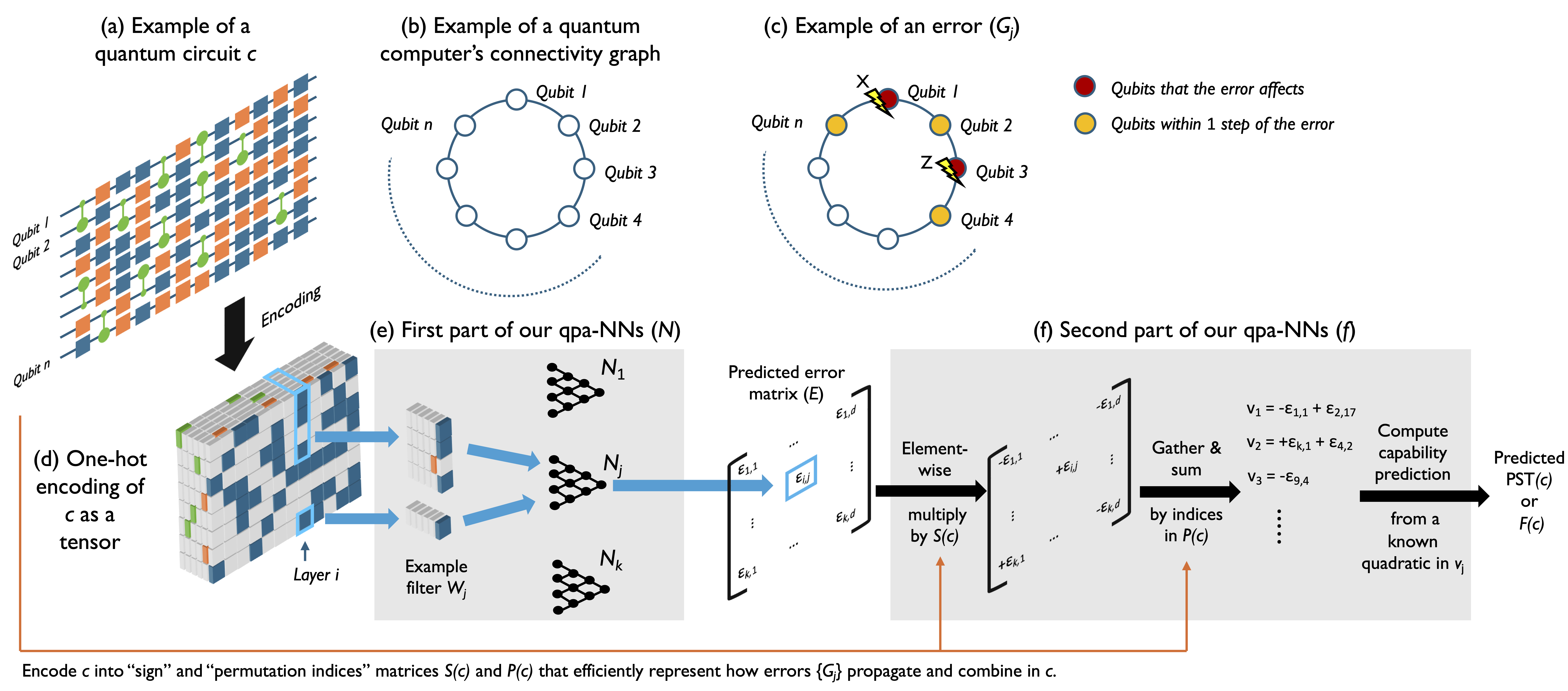
In this work, we introduce a novel quantum-physics-aware neural network (qpa-NN) architecture for quantum capability learning (Fig. 1). Our approach uses neural networks with GNN-inspired structures to predict the rates of the most physically relevant errors in quantum programs. These predicted error rates are then combined using an efficient approximation to the exact (but exponentially costly) quantum physics formula for how those errors combine to impact a program’s success rate. Our approach leverages the graph structures that encode the physics of how errors’ rates typically depend on both the quantum program being run and how a quantum computer’s qubits are arranged, and it offloads the difficult-to-learn, yet classically tractable task of approximately combining these error rates to predict a circuit’s performance to an already-known function. This enables our qpa-NNs to vastly outperform the state-of-the-art CNNs of Hothem et al. [2023c] on both experimental and simulated data.
Our qpa-NNs are enabled, in part, by focusing on learning a quantum computer’s capability on high-fidelity quantum programs, which are those programs that a quantum computer correctly executes with high probability. High-fidelity programs are arguably the most interesting programs to study as we care far more about whether a quantum computer successfully executes a program 99% or 90% of the time rather than 1% or 10% of the time.
In a head-to-head comparison, our qpa-NNs achieve a reduction in mean absolute error (MAE) over the CNNs of Hothem et al. [2023c], on average and on the same experimental datasets. Our qpa-NNs achieve an average improvement over those CNNs even after fine-tuning those CNNs on the same subset of the training data (high-fidelity programs) used to train our qpa-NNs.
Our qpa-NNs’ improved performance is likely largely due to their improved ability to model the impact of coherent errors on a program’s success rate. Off-the shelf networks struggle with coherent errors [Hothem et al., 2023c], but our qpa-NNs are designed to model how these errors add up and cancel out, making the qpa-NNs much better predictors in the presence of coherent errors. To verify this, we demonstrate that our qpa-NNs can accurately predict the performance of random circuits run on a hypothetical 4-qubit quantum computer experiencing only coherent errors. Our qpa-NN obtained a lower MAE than a CNN, averaged across five datasets, and the trained qpa-NN even exhibits moderate performance when making predictions for a different class of circuits (random mirror circuits [Proctor et al., 2021a]) simulated on the same hypothetical 4-qubit quantum computer, i.e., our qpa-NNs display moderate prediction accuracy on out-of-distribution data.
2 Background
In this section, we review the background in quantum computing necessary to understand this paper. See Nielsen and Chuang [2010] for an in-depth introduction to quantum computing and Blume-Kohout et al. [2022] for a thorough description of the errors in quantum computers.
2.1 Quantum computing
A quantum computer performs computations using qubits, which are two-level systems whose pure states are unit vectors in a complex two-dimensional Hilbert space, . The pure states of qubits are unit vectors in . The two orthonormal vectors and that are eigenvectors of the Pauli operator are identified as the computational basis of . Errors and noise in real quantum computers mean that they are typically in states that are probabilistic mixtures of pure states.
A quantum computation is performed by running a quantum program, typically known as a quantum circuit (see illustration in Fig. 1a). An -qubit quantum circuit () of depth is defined by a sequence of layers of logical instructions . Executing consists of preparing each qubit in , applying each , and then measuring each qubit to obtain an -bit string . Each layer typically consists of parallel one- and two-qubit gates, and it is intended to implement a unitary . Together, the layers are intended to implement .
If quantum circuit is implemented without error, its output bit string is a sample from a distribution whose probabilities are given by where , , and is the -th bit in . However, when a circuit is executed on a real quantum computer, errors can occur and this means that its output bit string is a sample from some other distribution . The process of errors corrupting a quantum computation can be modelled as follows. Each logic layer implements the intended unitary superoperator , where is a general -qubit state, followed by an error channel that is a completely positive and trace preserving (CPTP) superoperator [Blume-Kohout et al., 2022]. The imperfect implementation of a circuit is then simply , and the output bit string is with probability .
2.2 Quantum capability learning
Because quantum computers are error-prone, knowing which quantum circuits a particular quantum computer can execute with low error probability is important. Known as quantum capability learning [Proctor et al., 2021a, Hothem et al., 2023c], this task formally involves learning the mapping between a set of quantum circuits and some success metric quantifying how well runs on a quantum computer . In this work we consider a large class of circuits known as Clifford (or stabilizer) circuits [Aaronson and Gottesman, 2004], which are sufficient to enable quantum error correction [Campbell et al., 2017], and two widely-used success metrics: probability of successful trial (PST) (a.k.a., success probability) and the process fidelity (a.k.a. entanglement fidelity) [Hothem et al., 2023c, Nielsen, 2002].
PST is defined only for definite-outcome circuits, which are circuits whose output distribution has (if run without error) support on a single bit string, . For any such circuit , PST is defined as
| (1) |
In practice, is estimated by running the circuit times on and calculating
| (2) |
Process fidelity is defined for all circuits, and it quantifies how close the actual quantum evolution of the qubits is to the ideal unitary evolution. It is given by
| (3) |
Estimating is more complicated than estimating (it requires embedding into other circuits), but efficient methods exist [Proctor et al., 2022].
2.3 Modelling errors in quantum computers
Our qpa-NNs build in efficient approximations to the quantum physics of errors in quantum computers. They do so using the following parameterization of an error channel: . Here is the set of different Hamiltonian (H) and Stochastic (S) elementary error generators introduced by Blume-Kohout et al. [2022], and is the rate of error . Not every kind of error process can be represented in this form (e.g., amplitude damping, or non-Markovian errors), but this parameterization includes many of the most important kinds of errors in contemporary quantum computers. Each H and S error generator is indexed by a non-identity element of the -qubit Pauli group (). The Pauli operator indexing an H or S error indicates the qubits it impacts and its direction, e.g., the H error generator indexed by is a coherent error on the 1st qubit and it rotates that qubit around its axis.
Our qpa-NNs use approximate formulas for computing or from the rates of H and S errors, which we now review. Consider pushing each error channel to the end of the circuit and combining them together, i.e., we compute the error channel defined by . Then
| (4) |
where and are the rates of the -indexed and error generators, respectively, in ’s error channel , and is the set of -qubit Pauli operators containing at least one or . Similarly,
| (5) |
Equations (4) and (5) are good approximations for low-error circuits [Mądzik et al., 2022].
3 Neural network architecture
Our neural network architecture (see Fig. 1) for quantum capability learning combines neural network layers that have GNN-like structures with efficient approximations to the physics of errors in quantum computers. The overall action of our neural networks is to map an encoding of a circuit to a prediction for or . The same network can predict either or by simply toggling between two different output layers that have no trainable parameters. Our architecture is divided into two sequential parts. The first part of our architecture is a neural network that has the task of learning about the kinds and rates of errors that occur in quantum circuits. We use GNN-like structures within to embed physics knowledge for how those errors depend on the quantum circuit being run. The second part of our architecture is a function with no learnable parameters, that turns ’s output into a prediction for or .
3.1 Physics-aware neural networks for predicting errors in quantum circuits
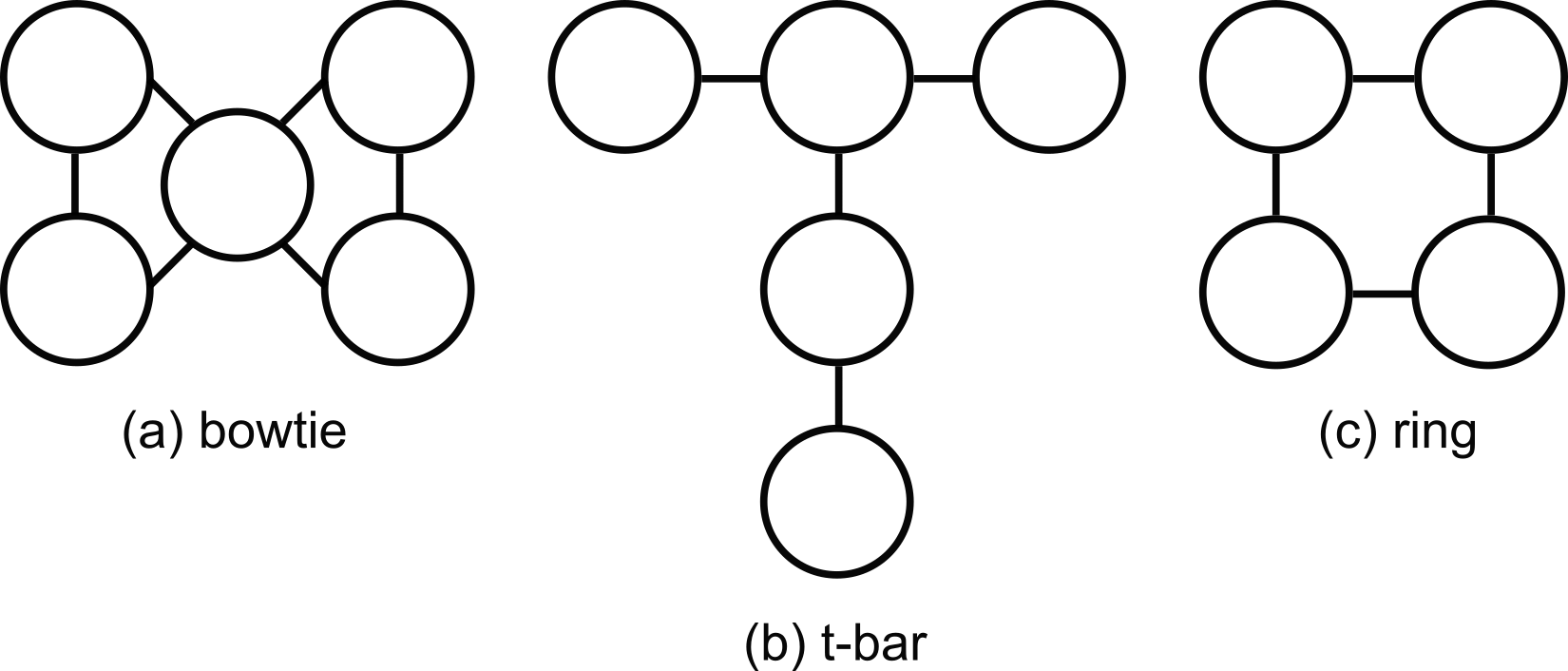
The neural network ’s input is a quantum circuit of depth represented by (i) a tensor describing the gates in (see Fig. 1a), and (ii) a matrix describing the measurement of the qubits at the end of . maps to a matrix and to a vector . is a prediction for the rate with which error type occurs during circuit layer , and is a prediction for the rate with which error type occurs when measuring the qubits at the end of a circuit. There are different possible error types that can occur in principle (see Section 2) so it is infeasible to predict all their rates beyond very small . However, the overwhelming majority of these errors are implausible, i.e., they are not expected to occur in real quantum computers [Blume-Kohout et al., 2022]. Our networks therefore predict the rates of every error from a relatively small set of error types containing the most plausible kinds of error. is a hyperparameter of our networks. It can be chosen to reflect the known physics of a particular quantum computer and/or optimized using hyperparameter tuning. In our demonstrations, we choose to contain all one-body H and S errors as well as all two-body H and S errors that interact pairs of qubits within steps on the modelled quantum computer’s connectivity graph for some constant (see Fig. 1b-c, where Fig. 1c shows an H or S error in if ). This choice for encodes the physical principles that errors are primarily either localized to a qubit or are two-body interactions between nearby qubits [Blume-Kohout et al., 2022]. The size of grows with , and for planar connectivity graphs (as in, e.g., contemporary superconducting qubit systems [Arute et al., 2019]) it grows linearly in . This results in errors whose rates must learn to predict.
The internal structures of are chosen to reflect general physical principles for how and depend on . is a prediction for the rate that occurs in circuit layer , and this error corresponds to a space/time location within —because it occurs at layer index or time and acts on a subset of the qubits (see example in Fig. 1c). This error’s rate will therefore primarily depend only on the gates in a time- and space-local region around its location in . Furthermore this dependence will typically be invariant under time translations (this is true except for some exotic non-Markovian kinds of errors, that we discuss in Section 7.1). We can encode these structures into by predicting from a space-time “window” of around the associated error’s location using a filter that “slides” across the circuit to predict the rate of versus time . Stated more formally, we predict using a multilayer perceptron whereby and is a snippet of whose temporal origin is (see Fig. 1e). The shape of each filter is a hyperparameter of our networks and it can be designed to reflect general physical principles, the known physics of a particular quantum computing system, and/or optimized with hyperparameter tuning. The particular neural networks we present later herein use filters that snip out only layer and discard the parts of the layer that act on qubits more than steps away from in the quantum computer’s connectivity graph (e.g., the filter shown in Fig. 1e corresponds to the error shown in Fig. 1c and ). This neural network structure has close connections to graph convolution layers [Kipf and Welling, 2016], as well as CNNs. We choose this structure as it can model spatially localized crosstalk errors, which are a ubiquitous but hard-to-model class of errors in quantum computers [Sarovar et al., 2020].
The network must also predict the rates of errors that occur during measurements (unless the qpa-NN will only ever predict not ), but these are typically independent of the rates of gate errors (which are predicted by the ). So we do not use the and their convolutional filters to make predictions for . Instead we use separate but structurally equivalent networks with corresponding filters that take as input and implement only spatial filtering. That is, simply discard rows from , as, unlike , has no temporal dimension. The are hyperparameters of our networks and we can separately adjust the shape of each to reflect the known physics of errors induced by measuring qubits. In our demonstrations, our filters have the same structure as the filters but with an independent steps parameter (large enables modelling many-qubit measurement crosstalk).
3.2 Processing predicted error rates to predict capabilities
We process ’s output to predict or using a function with no learnable parameters. This turns ’s output into the two quantities of interest, and it is also makes training feasible. We cannot easily train in isolation because the error matrix predicted by is not a directly observable quantity. Generating the data needed to train directly would require extraordinarily expensive quantum process tomography [Nielsen et al., 2021], which is infeasible except for very small . In contrast, both and can be efficiently estimated (see Section 2) for a given circuit .
The function computes an approximation to the value for or predicted by and . The matrix encodes the prediction that ’s imperfect action is
| (6) |
where the are the layers of (see Section 2) and , i.e., is an error channel parameterized by the th column of . Equation (6) implies an exact prediction for or [e.g., Eq. (3)], but exactly computing that prediction involves explicitly creating and multiplying together each of the matrices in Eq. (6). This is infeasible, except for very small . Instead our computes an efficient approximation to this prediction.
Our function ’s action is most easily described by embedding into the space of all possible H and S errors , resulting in a matrix whose columns are -sparse. However, we never construct these exponentially large matrices. Consider pulling each error channel to the end of the circuit, giving where . Because contains only Clifford gates and Clifford unitaries preserve the Pauli group [Aaronson and Gottesman, 2004], has columns that are just -dependent signed permutations of ’s columns. The signed permutations required can be efficiently computed in advance (i.e., as an input encoding step) using an efficient representation of Clifford unitaries [Gidney, 2021]. Furthermore, these permutations can be efficiently represented in two matrices: a sign matrix containing signs to be element-wise multiplied with and a permutation indices matrix containing integers between 1 and , where specifies what error becomes when pulled through the circuit layers after layer .
We now have a representation of ’s prediction for the circuit ’s error map as a sequence of error maps , and we need to predict or . We can do so if we can compute ’s prediction for the S and H error rates in , as we can then apply Eq. (4) or Eq. (5). To achieve this, we combine the into a single error map using a first-order Baker-Campbell-Hausdorff (BCH) expansion. Using our embedded representation, this means simply approximating as where , i.e., we sum over the rows of . To predict we then simply apply Eq. (4) (meaning summing up with those elements that correspond to Hamiltonian errors squared). Because measurement errors impact , to predict we again apply the BCH expansion to combine in the predicted measurement error map and then apply Eq. (5). The efficient representation of the overall action of is illustrated in Fig. 1 (the addition of the measurement error map is not shown).
4 Datasets
4.1 Experimental data
We used the 5-qubit datasets in Hothem et al. [2023c] for our experimental demonstrations. Each of these datasets was gathered by running random and periodic mirror circuits (two types of definite-outcome circuits) on 5-qubit IBM Q computers (, , , , and ), and estimating the PST of each circuit using Eq. (2). Each circuit was run between and times, with the exact number depending upon how many times the circuit sampling process generated the circuit (some short, -qubit circuits were generated multiple times). The random and periodic mirror circuits contained between and active qubits—called the circuit’s width—and ranged in depth from to layers (alt. for the dataset).
In this work we focus on high-PST circuits, so we removed all circuits with a PST less than from each dataset, leaving between () and 1369 () circuits in each dataset. The remaining circuits were partitioned into training, validation, and test sets based upon their original assignment in Hothem et al. [2023c]. This setup enables a direct comparison between our qpa-NNs and the CNNs trained in Hothem et al. [2023c]. Training set sizes ranged from circuits on to circuits on , with an approximate training, validation, testing split of , , and , respectively.
4.2 Simulated data
For our simulations, we generated 5 datasets of high-fidelity () random circuits, for a hypothetical 4-qubit processor with a “ring” geometry (i.e., like that in Fig. 1b). The circuits ranged in width () from to qubits, and in depth from 1 to 180 circuit layers. Each circuit was designed for a randomly chosen subset of qubits. Each circuit layer was created by i.i.d. sampling from all possible circuit layers on the active qubits. We used a gate set containing two-qubit gates and 7 different single-qubit gates (specifically where denotes a rotation around the axis by ). See Appendix C for additional details.
All circuits were simulated under the same error model, consisting of local coherent (i.e., H) errors, to exactly compute each ’s [Fig. 3 shows a histogram of ]. After removing duplicate circuits, the resulting datasets were partitioned into training, validation, and testing subsets, with a partition of , , and , respectively. The parameters of the error model were randomly selected: each gate was assigned a small error strength, which was then distributed randomly across all possible (local) one- or two-qubit coherent errors, for the one- and two-qubit gate, respectively. We chose a model with only coherent errors as these errors are ubiquitous, they are hard to model accurately and efficiently, and we conjecture that qpa-NNs can model them.
We also generated 5 datasets of 750 random mirror circuits on the same hypothetical quantum computer. Again, random mirror circuits varied in width from to qubits, and were designed to be run on a randomly selected subset of qubits. However, instead of i.i.d. sampling of each circuit layer, each circuit was randomly sampled from the class of random mirror circuits on the qubits. The depth of the mirror circuits ranged from 8 to 174 layers. We generated the mirror circuit datasets to evaluate how well qpa-NNs and CNNs generalize to out-of-distribution circuits, so they were used exclusively as testing sets. To ensure that no training was performed on mirror circuits, we removed any mirror circuits that appeared in the random circuit sets (in actuality, there were no duplicates).
4.3 Encoding schemes
We used two different encoding schemes for converting each circuit into a tensor. For the CNNs on experimental data, we used the same encoding scheme as Hothem et al. [2023c], as we used their data and networks. For all qpa-NNs, and the CNNs on simulated data, we used the following scheme. As outlined in Section 3, each width- circuit is represented by a three-dimensional tensor describing the gates in and a matrix describing the measurement of the qubits. The -th entry of ,
| (7) |
is a one-hot encoded vector of what happens to qubit in layer . For the hypothetical 4-qubit ring processor, : one channel for each single-qubit gate and four channels for the CNOT gates. There are four CNOT channels to specify if the qubit is the target or control qubit and if the interacting qubit is to the left or right of qubit . We used an additional 4 or 8 CNOT channels for the experimental data, depending on the quantum computer’s geometry. The first row in is the bitstring specifying which qubits are measured at the end of . When is a definite-outcome circuit, the second row is its target bit string, i.e., the sole bit string in the support of ’s outcome distribution when it is executed without error [i.e., ]. Both and are zero-padded to ensure a consistent tensor shape across a dataset.
Additionally, each circuit is accompanied by a permutation matrix and sign matrix . The -entry of specifies which error the -th tracked error occurring after the -th layer is transformed into at the end of the circuit. The -th entry of specifies the sign of that error.
5 Experiments
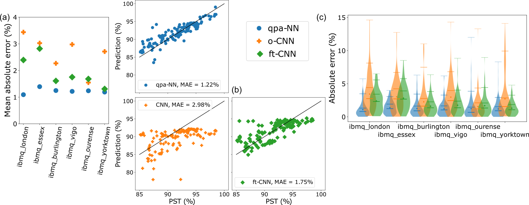
We now present the results from our head-to-head comparison between the qpa-NNs and the CNNs on the 5-qubit datasets used in Hothem et al. [2023c]. Figure 2 shows the mean absolute error (MAE) achieved by the CNNs () and the qpa-NNs () on each of the datasets. For all datasets, MAE is lower for the qpa-NNs than the CNN, with an average reduction of (, i.e., the standard deviation of percent-drop in MAE). The Bayes factor is between and (here, is the ratio of the likelihood of the qpa-NN to the likelihood of the CNN given the test data). This is overwhelming evidence that the qpa-NN is a better model ( is typically considered decisive). These results strongly suggest that the extra infrastructure in the qpa-NNs is making a difference.
The improved performance of the qpa-NNs is not because of an increase in model size. For example, the CNN contains trainable parameters compared to the trainable parameters in the qpa-NN. Moreover, CNNs of similar or larger sizes than the qpa-NNs were included in the hyperparameter optimization space of the CNNs [Hothem et al., 2023c].
Nonetheless, comparing the qpa-NNs to the CNNs is somewhat unfair as the CNNs were trained on out-of-distribution circuits—they were trained on the entire training dataset from Hothem et al. [2023c] which also contains low-PST circuits. For a fairer comparison, we fine-tuned each CNN (Fig. 2, ) on the same high-PST training set used to train the qpa-NNs. Fine-tuning typically increased the CNNs’ performances (mean improvement, ). However, the qpa-NNs achieve a MAE that is lower than the fine-tuned CNNs by on average () and outperform the fine-tuned CNNs on all six datasets. is between and , which is overwhelming evidence that the qpa-NNs are better models than the fine-tuned CNNs.
6 Simulations
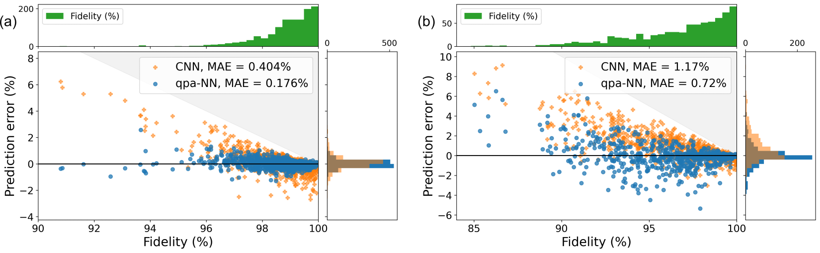
One reason why the extra infrastructure in our qpa-NNs may be necessary is that off-the-shelf networks struggle with modeling coherent errors [Hothem et al., 2023c]. To test our hypothesis, we trained a qpa-NN to predict the fidelity of random circuits executed on a hypothetical 4-qubit quantum computer experiencing purely coherent errors. We compared this qpa-NN to a hyperparameter-tuned CNN trained on the same data. Figure 3 shows the results from one representative dataset.
The qpa-NNs again significantly outperform the CNNs. Across the five datasets, the qpa-NNs’ averaged a reduction in MAE () on the test data. We also see a significant improvement in the mean Pearson correlation coefficient, vs. .
We also found that qpa-NNs trained on random circuits are modest predictors of the infidelity of random mirror circuits, which are a different family of circuits. This is an example of out-of-distribution generalization. Random mirror circuits differ in a variety of ways from the random circuits on which the qpa-NNs were trained, including both the presence of idle gates (which are noiseless in our simulations) and a motion-reversal structure in the circuits that causes the addition or cancellation of errors that are far apart in time. The qpa-NNs achieve an average MAE of on the random mirror circuits (). Although this is a increase in MAE over the in-distribution test data, the strong linear relation between the network’s predictions and the ground truth (, ) strongly suggests that the qpa-NNs are learning information relevant to random mirror circuits.
7 Discussion
7.1 Limitations
Our results are a significant improvement over the state of the art, but our approach does have several limitations:
-
1.
As presently conceived, our approach assumes that the modelled quantum computer’s error rates are invariant under time translations, which is a kind of Markovianity assumption (although it is weaker than the typical Markovian assumption used in conventional quantum computer models [Nielsen et al., 2021]). However, non-Markovian noise exists in quantum computers [White et al., 2020]. In the future, we plan to address this issue by adding temporal information into our approach, perhaps with a temporal or positional encoding [Vaswani et al., 2017].
-
2.
Our approach only considers two error classes (H and S errors). Other Markovian error classes, like amplitude damping, exist, but their error rates contribute to PST and fidelity at order [Mądzik et al., 2022]. Our approach can be easily extended to include those errors, if necessary, by learning their rates with and updating to account for their presence.
-
3.
Our current approach works for Clifford circuits, which includes arguably the most important kinds of circuits (e.g., quantum error correction circuits) but not all interesting circuits. This is because our method for efficiently propagating errors through circuits (implemented by together with the and matrices) leverages the elegant mathematics of Clifford circuits. Our approach can be easily extended to generic few-qubit quantum circuits ( qubits), but to obtain the efficiency needed for large with general circuits we will need to develop approximate methods for propagating errors through those circuits.
7.2 Conclusion
In this paper, we presented a new quantum-physics-aware neural network architecture for modelling a quantum computer’s capability that significantly improves upon the state of the art. The new architecture concatenates two parts: (i) a neural network with structural similarities to GNNs that uses gate information and a quantum computer’s connectivity graph to predict the rates of errors in each of a circuit’s layers, and (ii) a non-trainable function that turns the predicted error rates into a capability prediction. By imbuing these networks with knowledge about how errors occur and combine within a circuit, we are able to outperform state-of-the-art CNN-based capability models by on both experimental data and simulated data. We also provided evidence that our quantum-physics-aware networks are learning the true physical error rates, as they exhibit modest prediction accuracy when predicting the fidelity of out-of-distribution quantum circuits, which would enable our networks to also be used to diagnose the error processes occurring in a particular quantum computer (an important task known as characterization or tomography [Nielsen et al., 2021]).
Understanding which quantum circuits a quantum computer can run, and how well it can run them, is an important yet challenging component of understanding a quantum computer’s power. Given the complexity of the problem, neural networks are likely to play a large role in its solution. As our results demonstrate, our new physics-aware network architecture could play a critical role in building fast and reliable neural network-based capability models.
Acknowledgments and Disclosure of Funding
This material was funded in part by the U.S. Department of Energy, Office of Science, Office of Advanced Scientific Computing Research, Quantum Testbed Pathfinder Program, and by the Laboratory Directed Research and Development program at Sandia National Laboratories. T.P. acknowledges support from an Office of Advanced Scientific Computing Research Early Career Award. We acknowledge the use of IBM Quantum services for this work. The views expressed are those of the authors, and do not reflect the official policy or position of IBM or the IBM Quantum team.
Sandia National Laboratories is a multi-mission laboratory managed and operated by National Technology & Engineering Solutions of Sandia, LLC (NTESS), a wholly owned subsidiary of Honeywell International Inc., for the U.S. Department of Energy’s National Nuclear Security Administration (DOE/NNSA) under contract DE-NA0003525. This written work is authored by an employee of NTESS. The employee, not NTESS, owns the right, title and interest in and to the written work and is responsible for its contents. Any subjective views or opinions that might be expressed in the written work do not necessarily represent the views of the U.S. Government. The publisher acknowledges that the U.S. Government retains a non-exclusive, paid-up, irrevocable, world-wide license to publish or reproduce the published form of this written work or allow others to do so, for U.S. Government purposes. The DOE will provide public access to results of federally sponsored research in accordance with the DOE Public Access Plan.
References
- Aaronson and Gottesman [2004] S. Aaronson and D. Gottesman. Improved simulation of stabilizer circuits. Phys. Rev. A, 70(5):052328, Nov. 2004. ISSN 1050-2947. doi: 10.1103/PhysRevA.70.052328. URL https://link.aps.org/doi/10.1103/PhysRevA.70.052328.
- Abadi et al. [2015] M. Abadi, A. Agarwal, P. Barham, E. Brevdo, Z. Chen, C. Citro, G. S. Corrado, A. Davis, J. Dean, M. Devin, S. Ghemawat, I. Goodfellow, A. Harp, G. Irving, M. Isard, Y. Jia, R. Jozefowicz, L. Kaiser, M. Kudlur, J. Levenberg, D. Mané, R. Monga, S. Moore, D. Murray, C. Olah, M. Schuster, J. Shlens, B. Steiner, I. Sutskever, K. Talwar, P. Tucker, V. Vanhoucke, V. Vasudevan, F. Viégas, O. Vinyals, P. Warden, M. Wattenberg, M. Wicke, Y. Yu, and X. Zheng. TensorFlow: Large-scale machine learning on heterogeneous systems, 2015. URL http://tensorflow.org/. Software available from tensorflow.org.
- [3] A. Anonymous. Supplemental code and data. . To be released. See attached anonymized zip file.
- Arute et al. [2019] F. Arute, K. Arya, R. Babbush, D. Bacon, J. C. Bardin, R. Barends, R. Biswas, S. Boixo, F. G. S. L. Brandao, D. A. Buell, B. Burkett, Y. Chen, Z. Chen, B. Chiaro, R. Collins, W. Courtney, A. Dunsworth, E. Farhi, B. Foxen, A. Fowler, C. Gidney, M. Giustina, R. Graff, K. Guerin, S. Habegger, M. P. Harrigan, M. J. Hartmann, A. Ho, M. Hoffmann, T. Huang, T. S. Humble, S. V. Isakov, E. Jeffrey, Z. Jiang, D. Kafri, K. Kechedzhi, J. Kelly, P. V. Klimov, S. Knysh, A. Korotkov, F. Kostritsa, D. Landhuis, M. Lindmark, E. Lucero, D. Lyakh, S. Mandrà, J. R. McClean, M. McEwen, A. Megrant, X. Mi, K. Michielsen, M. Mohseni, J. Mutus, O. Naaman, M. Neeley, C. Neill, M. Y. Niu, E. Ostby, A. Petukhov, J. C. Platt, C. Quintana, E. G. Rieffel, P. Roushan, N. C. Rubin, D. Sank, K. J. Satzinger, V. Smelyanskiy, K. J. Sung, M. D. Trevithick, A. Vainsencher, B. Villalonga, T. White, Z. J. Yao, P. Yeh, A. Zalcman, H. Neven, and J. M. Martinis. Quantum supremacy using a programmable superconducting processor. Nature, 574(7779):505–510, Oct. 2019. ISSN 0028-0836, 1476-4687. doi: 10.1038/s41586-019-1666-5. URL http://dx.doi.org/10.1038/s41586-019-1666-5.
- Blume-Kohout et al. [2022] R. Blume-Kohout, M. P. da Silva, E. Nielsen, T. Proctor, K. Rudinger, M. Sarovar, and K. Young. A taxonomy of small markovian errors. PRX Quantum, 3:020335, May 2022. doi: 10.1103/PRXQuantum.3.020335. URL https://link.aps.org/doi/10.1103/PRXQuantum.3.020335.
- Campbell et al. [2017] E. T. Campbell, B. M. Terhal, and C. Vuillot. Roads towards fault-tolerant universal quantum computation. Nature, 549(7671):172–179, Sept. 2017. ISSN 0028-0836, 1476-4687. doi: 10.1038/nature23460. URL http://dx.doi.org/10.1038/nature23460.
- Cao et al. [2019] Y. Cao, J. Romero, J. P. Olson, M. Degroote, P. D. Johnson, M. Kieferová, I. D. Kivlichan, T. Menke, B. Peropadre, N. P. D. Sawaya, S. Sim, L. Veis, and A. Aspuru-Guzik. Quantum chemistry in the age of quantum computing. Chemical Reviews, 119(19):10856–10915, 2019. doi: 10.1021/acs.chemrev.8b00803. URL https://doi.org/10.1021/acs.chemrev.8b00803. PMID: 31469277.
- Chollet et al. [2015] F. Chollet et al. Keras. https://keras.io, 2015.
- Elsayed Amer et al. [2022] N. Elsayed Amer, W. Gomaa, K. Kimura, K. Ueda, and A. El-Mahdy. On the learnability of quantum state fidelity. EPJ Quantum Technology, 9:31, 2022. URL https://epjquantumtechnology.springeropen.com/articles/10.1140/epjqt/s40507-022-00149-8#citeas.
- Gidney [2021] C. Gidney. Stim: a fast stabilizer circuit simulator. Quantum, 5:497, July 2021. ISSN 2521-327X. doi: 10.22331/q-2021-07-06-497. URL https://doi.org/10.22331/q-2021-07-06-497.
- Harrow et al. [2009] A. W. Harrow, A. Hassidim, and S. Lloyd. Quantum algorithm for linear systems of equations. Phys. Rev. Lett., 103:150502, Oct 2009. doi: 10.1103/PhysRevLett.103.150502. URL https://link.aps.org/doi/10.1103/PhysRevLett.103.150502.
- Hothem et al. [2023a] D. Hothem, T. Catanach, K. Young, and T. Proctor. Learning a quantum computer’s capability using convolutional neural networks [Data set]. https://doi.org/10.5281/zenodo.7829489, 2023a. Published: 2023-04-12.
- Hothem et al. [2023b] D. Hothem, J. Hines, K. Nataraj, R. Blume-Kohout, and T. Proctor. Predictive models from quantum computer benchmarks. In 2023 IEEE International Conference on Quantum Computing and Engineering (QCE), pages 709–714, Los Alamitos, CA, USA, sep 2023b. IEEE Computer Society. doi: 10.1109/QCE57702.2023.00086. URL https://doi.ieeecomputersociety.org/10.1109/QCE57702.2023.00086.
- Hothem et al. [2023c] D. Hothem, K. Young, T. Catanach, and T. Proctor. Learning a quantum computer’s capability using convolutional neural networks, 2023c. URL https://arxiv.org/abs/2304.10650.
- Kingma and Ba [2015] D. Kingma and J. Ba. Adam: A method for stochastic optimization. In Y. Bengio and Y. LeCun, editors, Proceedings of the 3rd International Conference for Learning Representations. Microtome, 2015. URL https://arxiv.org/abs/1412.6980.
- Kipf and Welling [2016] T. N. Kipf and M. Welling. Semi-Supervised classification with graph convolutional networks. Sept. 2016. URL http://arxiv.org/abs/1609.02907.
- Lubinski et al. [2023] T. Lubinski, S. Johri, P. Varosy, J. Coleman, L. Zhao, J. Necaise, C. H. Baldwin, K. Mayer, and T. Proctor. Application-Oriented performance benchmarks for quantum computing. IEEE Transactions on Quantum Engineering, 4:1–32, 2023. ISSN 2689-1808. doi: 10.1109/TQE.2023.3253761. URL http://dx.doi.org/10.1109/TQE.2023.3253761.
- Mądzik et al. [2022] M. T. Mądzik, S. Asaad, A. Youssry, B. Joecker, K. M. Rudinger, E. Nielsen, K. C. Young, T. J. Proctor, A. D. Baczewski, A. Laucht, V. Schmitt, F. E. Hudson, K. M. Itoh, A. M. Jakob, B. C. Johnson, D. N. Jamieson, A. S. Dzurak, C. Ferrie, R. Blume-Kohout, and A. Morello. Precision tomography of a three-qubit donor quantum processor in silicon. Nature, 601(7893):348–353, Jan. 2022.
- Nielsen et al. [2020] E. Nielsen, K. Rudinger, T. Proctor, A. Russo, K. Young, and R. Blume-Kohout. Probing quantum processor performance with pyGSTi. Quantum Sci. Technol., 5(4):044002, July 2020. ISSN 2058-9565. doi: 10.1088/2058-9565/ab8aa4. URL https://iopscience.iop.org/article/10.1088/2058-9565/ab8aa4.
- Nielsen et al. [2021] E. Nielsen, J. K. Gamble, K. Rudinger, T. Scholten, K. Young, and R. Blume-Kohout. Gate set tomography. Quantum, 5(557):557, Oct. 2021. ISSN 2521-327X. doi: 10.22331/q-2021-10-05-557. URL https://quantum-journal.org/papers/q-2021-10-05-557/.
- Nielsen [2002] M. A. Nielsen. A simple formula for the average gate fidelity of a quantum dynamical operation. Physics Letters A, 303(4):249–252, 2002.
- Nielsen and Chuang [2010] M. A. Nielsen and I. L. Chuang. Quantum Computation and Quantum Information: 10th Anniversary Edition. Cambridge University Press, 2010.
- Proctor et al. [2021a] T. Proctor, K. Rudinger, K. Young, E. Nielsen, and R. Blume-Kohout. Measuring the capabilities of quantum computers. Nature Phys, 18(1):75, Dec. 2021a. ISSN 1745-2473. doi: 10.1038/s41567-021-01409-7. URL https://www.nature.com/articles/s41567-021-01409-7.
- Proctor et al. [2021b] T. Proctor, K. Rudinger, K. Young, E. Nielsen, and R. Blume-Kohout. Scalable randomized benchmarking of quantum computers using mirror circuits [Data set]. https://doi.org/10.5281/zenodo.5197499, 2021b. Accessed: 2023-04-12.
- Proctor et al. [2022] T. Proctor, S. Seritan, E. Nielsen, K. Rudinger, K. Young, R. Blume-Kohout, and M. Sarovar. Establishing trust in quantum computations, 2022. URL https://arxiv.org/abs/2204.07568.
- Rubin et al. [2023] N. Rubin, D. Berry, A. Kononov, F. Malone, T. Khattar, A. White, J. Lee, H. Neven, R. Babbush, and A. Baczewski. Quantum computation of stopping power for inertial fusion target design. arXiv preprint, 2023. URL https://arxiv.org/abs/2308.12352.
- Sarovar et al. [2020] M. Sarovar, T. Proctor, K. Rudinger, K. Young, E. Nielsen, and R. Blume-Kohout. Detecting crosstalk errors in quantum information processors. Quantum, 4(321):321, Sept. 2020. ISSN 2521-327X. doi: 10.22331/q-2020-09-11-321. URL https://quantum-journal.org/papers/q-2020-09-11-321/.
- Shor [1997] P. W. Shor. Polynomial-time algorithms for prime factorization and discrete logarithms on a quantum computer. SIAM Journal on Computing, 26(5):1484–1509, 1997. doi: 10.1137/S0097539795293172. URL https://doi.org/10.1137/S0097539795293172.
- Vadali et al. [2024] A. Vadali, R. Kshirsagar, P. Shyamsundar, and G. N. Perdue. Quantum circuit fidelity estimation using machine learning. Quantum Mach. Intell., 6(1), June 2024.
- Vaswani et al. [2017] A. Vaswani, N. Shazeer, N. Parmar, J. Uszkoreit, L. Jones, A. N. Gomez, L. Kaiser, and I. Polosukhin. Attention is all you need. In Proceedings of the 31st International Conference on Neural Information Processing Systems, NIPS’17, page 6000–6010, Red Hook, NY, USA, 2017. Curran Associates Inc. ISBN 9781510860964.
- Wang et al. [2022] H. Wang, P. Liu, J. Cheng, Z. Liang, J. Gu, Z. Li, Y. Ding, W. Jiang, Y. Shi, X. Qian, et al. Quest: Graph transformer for quantum circuit reliability estimation. arXiv preprint arXiv:2210.16724, 2022.
- White et al. [2020] G. A. L. White, C. D. Hill, F. A. Pollock, L. C. L. Hollenberg, and K. Modi. Demonstration of non-markovian process characterisation and control on a quantum processor. Nature Communications, 11(1), Dec. 2020. ISSN 2041-1723. doi: 10.1038/s41467-020-20113-3. URL http://dx.doi.org/10.1038/s41467-020-20113-3.
Appendix A Compute resources
All of the quantum-physics-aware neural networks were trained using a 6-Core Intel Core i9 processor on a MacBookPro 15.1 with 32GB of memory. Each model took roughly 15-20 wall clock minutes to train. Total training time, across the paper, totaled wall clock minutes.
All of the simulations and data pre-processing were performed using a 6-core Intel Core i9 processor on a MacBookPro 15.1 with 32GB of memory. Each dataset took approximately 1 hour of wall clock time to create. This total includes the initial circuit creation, simulating the circuits, and encoding each circuit into a tensor.
Appendix B Code and data availability
The simulated 5-qubit data as well as records of all the quantum physics-aware networks can be found in Anonymous . The CNNs and 5-qubit experimental datasets used in Hothem et al. [2023c] are available at Hothem et al. [2023a]. The datasets were originally located at Proctor et al. [2021b]. Each dataset was released under a CC-BY 4.0 International license.
All simulations were performed using a combination of version 0.9.11.2 [Nielsen et al., 2020] and version 1.13.0 [Gidney, 2021]. Models were trained and developed using version 2.12.0 [Chollet et al., 2015] and version 2.12.0 [Abadi et al., 2015]. The physics-aware network model classes ( for PST and for process fidelity) are available in the Supplementary Material.
Appendix C Datasets
| Device | Geometry | Circuit types | Circuit widths | Circuit depths | Training set size | Validation set size | Test set size |
|---|---|---|---|---|---|---|---|
| ibmq_london | t-bar | mirror | 1-5 qubits | 3-515 layers | 711 circuits | 104 circuits | 91 circuits |
| ibmq_ourense | t-bar | mirror | 1-5 qubits | 3-515 layers | 930 circuits | 124 circuits | 114 circuits |
| ibmq_essex | t-bar | mirror | 1-5 qubits | 3-515 layers | 713 circuits | 93 circuits | 86 circuits |
| ibmq_burlington | t-bar | mirror | 1-5 qubits | 3-515 layers | 682 circuits | 90 circuits | 92 circuits |
| ibmq_vigo | t-bar | mirror | 1-5 qubits | 3-515 layers | 1029 circuits | 137 circuits | 126 circuits |
| ibmq_yorktown | bowtie | mirror | 1-5 qubits | 3-515 layers | 1097 circuits | 132 circuits | 140 circuits |
| Ring (x5) | ring | random i.i.d. | 1-4 qubits | 1-180 layers | 2813 circuits | 938 circuits | 1250 circuits |
| Ring (x5) | ring | mirror | 1-4 qubits | 8-174 layers | - | - | 750 circuits |
We provide additional details on the datasets used in the paper. Table 1 summarizes each dataset. We tracked all weight- errors with support on qubits connected by hops in all the datasets. Below, we provide additional details on the circuit and error model generating processes.
C.1 Creating the circuits
In this subsection, we go over how the random i.i.d.-layer circuits and random mirror circuits were created for this paper. We start by explaining how we generated the random i.i.d.-layer circuits for a 4-qubit ring processor, and then explain the modifications needed to generate the random mirror circuits. This subsection’s content is conceptual. The actual circuits were created in using the code in the Supplementary Material.
Each random i.i.d.-layer circuit was created by a multi-step process. First, we randomly sampled a connected subset of qubits for which is designed for. Then, we uniformly sampled ’s depth from between and , a pre-determined, circuit-width-dependent maximum depth. The depths were selected to ensure that given the maximum error strengths used to create the simulated error model (Section C.2). Third, we randomly sampled a two-qubit gate density between and . The density determines the average number of two-qubit gates in each of ’s layers. We then sampled each layer i.i.d. from all possible circuit layers on the qubits in .
The random mirror circuits were generated using a similar multi-step process with two differences. The first difference is that we used a pre-determined maximum depth of . We chose to reduce the pre-determined, circuit-width-dependent maximum depth so that the deepest random mirror circuits had roughly the same length as the deepest random i.i.d. circuits. The second difference is that we created a random mirror circuit on . See Proctor et al. [2021a] for more details.
C.2 Creating an error model
In this subsection, we explain how we constructed the -qubit Markovian local coherent error model used in Section 6. Again, we provide a conceptual explanation. The actual error model was created in using the code found in the Supplementary Material.
The -qubit Markovian local coherent error model was specified using the error generator framework explained in Section 2 and Blume-Kohout et al. [2022]. The error model consists of operation-dependent errors sampled according to a two-step process. The error strengths for each gate and qubit(s) pairs were independently sampled. First, we sampled an overall error strength for each one- and two-qubit gate by randomly sampling from and scaling by a pre-determined maximum error strength (). Then we sampled the relative error strengths of each of the coherent errors, where for one- and two-qubit gates, respectively. We then normalized to obtain the actual error strengths according to the following equation:
| (8) |
The re-scaling ensures that, to first order, gate contributes approximately to the circuit’s process infidelity (or PST, if appropriate).
Appendix D Networks
D.1 Quantum-physics-aware network details
| Dataset | Metric | Model size | Dense units | ||
|---|---|---|---|---|---|
| -qubit t-bar | [30, 20, 10, 5, 5, 1] | ||||
| -qubit bowtie | [30, 20, 10, 5, 5, 1] | ||||
| -qubit ring | [30, 20, 10, 5, 5, 1] |
Table 2 briefly outlines the hyperparameters and model sizes of the physics-aware neural networks used in this paper. The and hyperparameters were chosen by hand based upon subject-matter-expert knowledge of the errors in a quantum computer. The size and shape of the dense layers were selected arbitrarily. All dense subunits used a activation function. All models were trained using ’s Adam [Kingma and Ba, 2015] optimizer with a step size of and with mean squared error as the loss function. Model training was cut short using early stopping. To help with training, we scaled and by 10000 when training the physics-aware networks. The notebooks in the Supplementary Material contain more details.
D.2 Convolutional neural network details
Details on the specific convolutional neural networks used in this paper are located in Hothem et al. [2023c]. We fine-tuned each network on high-PST experimental data using the Adam optimizer and early stopping.
We selected the model architecture for the convolutional neural networks used in our simulations via hyperparameter tuning. We performed 100 trials of hyperparameter tuning using the class in . Additional details, including the specific hyperparameter space, are located in the Supplementary Material.
Appendix E Experimental results
| Dataset | Network | Mean absolute error (%) | Bayes factor vs. CNN | Bayes factor vs. ft-CNN |
|---|---|---|---|---|
| ibmq_london | qpa-NN | 1.09 | ||
| CNN | 3.44 | - | - | |
| ft-CNN | 2.39 | - | ||
| ibmq_ourense | qpa-NN | 1.24 | ||
| CNN | 1.55 | - | - | |
| ft-CNN | 1.68 | - | ||
| ibmq_essex | qpa-NN | 1.39 | ||
| CNN | 3.03 | - | - | |
| ft-CNN | 2.82 | - | ||
| ibmq_burlington | qpa-NN | 1.25 | ||
| CNN | 2.27 | - | - | |
| ft-CNN | 1.61 | |||
| ibmq_vigo | qpa-NN | 1.21 | ||
| CNN | 2.98 | - | - | |
| ft-CNN | 1.75 | - | ||
| ibmq_yorktown | qpa-NN | 1.19 | ||
| CNN | 2.71 | - | - | |
| ft-CNN | 1.31 | - |
Table 3 summarizes model performance on each of the experimental datasets used in the paper. Copies of the pre-trained quantum-physics-aware neural networks, original CNNs, and fine-tuned CNNs are available in the Supplementary Material. Scatter plots of each model’s predictions are also available in the Supplementary Material.
Appendix F Simulation results
| Dataset | Network | Circuit type | Mean absolute error (%) | Pearson correlation coefficient |
|---|---|---|---|---|
| 0 | qpa-NN | random i.i.d. | .176 | .968 |
| mirror | .720 | .914 | ||
| CNN | random i.i.d. | .404 | .751 | |
| mirror | 1.17 | .872 | ||
| 1 | qpa-NN | random i.i.d. | .200 | .960 |
| mirror | .652 | .921 | ||
| CNN | random i.i.d. | .421 | .741 | |
| mirror | .922 | .861 | ||
| 2 | qpa-NN | random i.i.d. | .190 | .970 |
| mirror | .769 | .914 | ||
| CNN | random i.i.d. | .406 | .732 | |
| mirror | 1.20 | .853 | ||
| 3 | qpa-NN | random i.i.d. | .191 | .952 |
| mirror | .719 | .912 | ||
| CNN | random i.i.d. | .367 | .764 | |
| mirror | 1.02 | .857 | ||
| 4 | qpa-NN | random i.i.d. | .195 | .960 |
| mirror | .761 | .898 | ||
| CNN | random i.i.d. | .405 | .763 | |
| mirror | 1.05 | .847 |
Table 4 summarizes model performance on each of the simulated datasets used in the paper. Copies of the pre-trained quantum-physics-aware neural networks and fine-tuned CNNs are available in the Supplementary Material. Scatter plots of each model’s prediction errors are also available in the Supplementary Material.