When are Kalman-Filter Restless Bandits Indexable?

We study the problem of monitoring several time series so as to maintain a precise belief while minimising the cost of sensing. Such problems can be viewed as POMDPs with belief-dependent rewards [3] and their applications include active sensing [7], attention mechanisms for multiple-object tracking [22], as well as online summarisation of massive data from time-series [4]. Specifically, we discuss the restless bandit [24] associated with the discrete-time Kalman filter [19].

Restless bandits generalise bandit problems [6, 8] to situations where the state of each arm (project, site or target) continues to change even if the arm is not played. As with bandit problems, the states of the arms evolve independently given the actions taken, suggesting that there might be efficient algorithms for large-scale settings, based on calculating an index for each arm, which is a real number associated with the (belief-)state of that arm alone. However, while bandits always have an optimal index policy (select the arm with the largest index), it is known that no index policy can be optimal for some discrete-state restless bandits [17] and such problems are in general PSPACE-hard even to approximate to any non-trivial factor [10]. Further, in this paper we address restless bandits with real-valued rather than discrete states.

On the other hand, Whittle proposed a natural index policy for restless bandits [24], but this policy only makes sense when the restless bandit is indexable, as we now explain. Say we have $n$ restless bandits and we are constrained to play $m$ arms at each time. Whittle considered relaxing this constraint by only requiring that the time-average number of arms played is $m$. Now the optimal average cost for this relaxed problem is a lower bound on the optimal average cost for the original problem. Also, the relaxed problem can be separated into $n$ single-arm problems by the method of Lagrange multipliers, making it relatively easy to solve. In this separated version of the relaxed problem, each arm behaves identically to an arm in the original problem, except that an additional price $\lambda$ is charged each time the arm is played, where $\lambda$ corresponds to the Lagrange multiplier for the relaxed constraint. Now let us consider a family of optimal policies which achieves the optimal cost-to-go $Q_{i}(x,u;\lambda)$ for a single arm $i$ with price $\lambda$ and which takes actions $u=\pi_{i}(x;\lambda)$ when in state $x$ where $u=0$ means passive and $u=1$ means active. At first glance, we might intuitively suppose that it becomes less and less attractive to be active as the price $\lambda$ increases so that as the price is increased beyond some value $\lambda_{i}(x)$, the optimal action switches from active to passive. At this price we are ambivalent between being active and passive so that $Q_{i}(x,0;\lambda_{i}(x))=Q_{i}(x,1;\lambda_{i}(x))$. Such a value $\lambda_{i}(x)$ is called the Whittle index for arm $i$ in state $x$. Indeed if there is a family of optimal policies for which

$\displaystyle\pi_{i}(x;\lambda_{\text{hi}})\leq\pi_{i}(x;\lambda_{\text{lo}})\quad\text{for all states $x$ and all pairs of prices $\lambda_{\text{hi}}\geq\lambda_{\text{lo}}$}$

then an optimal solution to the relaxed problem for price $\lambda$ is to activate arm $i$ if and only if $\lambda<\lambda_{i}(x)$. If a restless bandit satisfies this condition, it is said to be indexable. It is important to note that some restless bandits are not indexable, so activating arm $i$ if and only if $\lambda<\lambda_{i}(x)$ does not correspond to an optimal solution to the relaxed problem. Indeed, in a study of small randomly-generated problems, Weber and Weiss [23] found that roughly 10% of problems were not indexable.

As a policy based on $\lambda_{i}(x)$ is so good for the relaxed problem when the arms are indexable, this motivates us to use $\lambda_{i}(x)$ as a heuristic for the original problem. This heuristic is called Whittle’s index policy and at each time it activates the $m$ arms with the highest indexes $\lambda_{i}(x)$. Further motivation for studying indexability is that for ordinary bandits the Whittle index reduces to the Gittins index, making the Whittle index policy optimal when only one arm may be active at each time, that is when $m=1$. More generally, Whittle’s index policy is not optimal for some restless bandit problems even when the arms are indexable, but indexability is still a rather useful concept, since if all arms are indexable and certain other conditions hold, Whittle’s policy is asymptotically optimal, as we now explain. Consider a sequence of restless bandit problems parameterised by the number of indexable arms $n$ and in which $m=\alpha n$ of the arms can be simultaneously active for some fixed $\alpha\in(0,1)$. Then as $n$ tends to infinity, the time-average cost per arm for Whittle’s index policy converges to the time-average cost per arm for an optimal policy, provided a certain fluid approximation has a unique fixed point. This result was first demonstrated by Weber and Weiss [23] who for simplicity of exposition only considered the symmetric case in which the $n$ arms have identical costs and transition probabilities. Recently, Verloop [20] extended this result to asymmetric cases involving multiple types of arms. Interestingly, this extension also covers cases where new arms arrive and old arms depart.

Restless bandits associated with scalar Kalman(-Bucy) filters in continuous time were recently shown to be indexable [12] and the corresponding discrete-time problem has attracted considerable attention over a long period [15, 11, 16, 21]. However, that attention has produced no satisfactory proof of indexability – even for scalar time-series and even if we assume that there is a monotone optimal policy for the single-arm problem, which is a policy that plays the arm if and only if the relevant belief-state exceeds some threshold (here the relevant belief-state is a posterior variance). Theorem 1 of this paper addresses that gap. After formalising the problem (Section 2), we describe the concepts and intuition (Section 3) behind the main result (Section 4). The main tools are mechanical words (which are not sufficiently well-known) and Schur convexity. As these tools are associated with rather general theorems, we believe that future work (Section 5) should enable substantial generalisation of our results.

We consider the problem of tracking $N$ time-series, which we call arms, in discrete time. The state $Z_{i,t}\in\mathbb{R}$ of arm $i$ at time $t\in\mathbb{Z}_{+}$ evolves as a standard-normal random walk independent of everything but its immediate past ($\mathbb{Z}_{+},\mathbb{R}_{-}$ and $\mathbb{R}_{+}$ all include zero). The action space is $\mathcal{U}:=\{1,\dots,N\}$. Action $u_{t}=i$ makes an expensive observation $Y_{i,t}$ of arm $i$ which is normally-distributed about $Z_{i,t}$ with precision $b_{i}\in\mathbb{R}_{+}$ and we receive cheap observations $Y_{j,t}$ of each other arm $j$ with precision $a_{j}\in\mathbb{R}_{+}$ where $a_{j}<b_{j}$ and $a_{j}=0$ means no observation at all.

Let $Z_{t},Y_{t},\mathcal{H}_{t},\mathcal{F}_{t}$ be the state, observation, history and observed history, so that $Z_{t}:=(Z_{1,t},\dots,Z_{N,t}),Y_{t}:=(Y_{1,t},\dots,Y_{N,t}),\mathcal{H}_{t}:=((Z_{0},u_{0},Y_{0}),\dots,(Z_{t},u_{t},Y_{t}))$ and $\mathcal{F}_{t}:=((u_{0},Y_{0}),\dots,(u_{t},Y_{t})).$ Then we formalise the above as (${\bf 1}_{\cdot}$ is the indicator function)

$\displaystyle Z_{i,0}$

$\displaystyle\sim\mathcal{N}(0,1),$

$\displaystyle Z_{i,t+1}\mid\mathcal{H}_{t}$

$\displaystyle\sim\mathcal{N}(Z_{i,t},1),$

$\displaystyle Y_{i,t}\mid\mathcal{H}_{t-1},Z_{t},u_{t}$

$\displaystyle\sim\mathcal{N}\left(Z_{i,t},\frac{{\bf 1}_{u_{t}\neq i}}{a_{i}}+\frac{{\bf 1}_{u_{t}=i}}{b_{i}}\right).$

Note that this setting is readily generalised to $\mathbb{E}[(Z_{i,t+1}-Z_{i,t})^{2}]\neq 1$ by a change of variables.

Thus the posterior belief is given by the Kalman filter as $Z_{i,t}\mid\mathcal{F}_{t}\sim\mathcal{N}(\hat{Z}_{i,t},x_{i,t})$ where the posterior mean is ${\hat{Z}}_{i,t}\in\mathbb{R}$ and the error variance $x_{i,t}\in\mathbb{R}_{+}$ satisfies

$\displaystyle x_{i,t+1}=\phi_{i,{\bf 1}_{u_{t+1}=i}}(x_{i,t})\quad\text{where}\quad\phi_{i,0}(x):=\frac{x+1}{a_{i}x+a_{i}+1}\ \ \text{and}\ \ \phi_{i,1}(x):=\frac{x+1}{b_{i}x+b_{i}+1}.$

(1)

Problem KF1. Let $\pi$ be a policy so that $u_{t}=\pi(\mathcal{F}_{t-1})$. Let $x^{\pi}_{i,t}$ be the error variance under $\pi$. The problem is to choose $\pi$ so as to minimise the following objective for discount factor $\beta\in[0,1)$. The objective consists of a weighted sum of error variances $x^{\pi}_{i,t}$ with weights $w_{i}\in\mathbb{R}_{+}$ plus observation costs $h_{i}\in\mathbb{R}_{+}$ for $i=1,\dots,N$:

$\displaystyle\mathbb{E}\left[\sum_{t=0}^{\infty}\sum_{i=1}^{N}\beta^{t}\left\{h_{i}{\bf 1}_{u_{t}=i}+w_{i}x_{i,t}^{\pi}\right\}\right]=\sum_{t=0}^{\infty}\sum_{i=1}^{N}\beta^{t}\left\{h_{i}{\bf 1}_{u_{t}=i}+w_{i}x_{i,t}^{\pi}\right\}$

where the equality follows as (1) is a deterministic mapping (and assuming $\pi$ is deterministic).

Single-Arm Problem and Whittle Index. Now fix an arm $i$ and write $x_{t}^{\pi},\phi_{0}(\cdot),\dots$ instead of $x_{t,i}^{\pi},\phi_{i,0}(\cdot),\dots$. Say there are now two actions $u_{t}=0,1$ corresponding to cheap and expensive observations respectively and the expensive observation now costs $h+\nu$ where $\nu\in\mathbb{R}$. The single-arm problem is to choose a policy, which here is an action sequence, $\pi:=(u_{0},u_{1},\dots)$

$\displaystyle\text{so as to minimise}\quad V^{\pi}(x|\nu):=\sum_{t=0}^{\infty}\beta^{t}\left\{(h+\nu)u_{t}+wx_{t}^{\pi}\right\}\quad\text{where $x_{0}=x$.}$

(2)

Let $Q(x,\alpha|\nu)$ be the optimal cost-to-go in this problem if the first action must be $\alpha$ and let $\pi^{*}$ be an optimal policy, so that

$\displaystyle Q(x,\alpha|\nu):=(h+\nu)\alpha+wx+\beta V^{\pi^{*}}(\phi_{\alpha}(x)|\nu).$

For any fixed $x\in\mathbb{R}_{+}$, the value of $\nu$ for which actions $u_{0}=0$ and $u_{0}=1$ are both optimal is known as the Whittle index $\lambda^{W}(x)$ assuming it exists and is unique. In other words

The Whittle index $\lambda^{W}(x)$ is the solution to $Q(x,0|\lambda^{W}(x))=Q(x,1|\lambda^{W}(x)).$

(3)

Let us consider a policy which takes action $u_{0}=\alpha$ then acts optimally producing actions $u_{t}^{\alpha*}(x)$ and error variances $x_{t}^{\alpha*}(x)$. Then (3) gives

$\displaystyle\sum_{t=0}^{\infty}\beta^{t}\left\{(h+\lambda^{W}(x))u^{0*}_{t}+wx_{t}^{0*}(x)\right\}=\sum_{t=0}^{\infty}\beta^{t}\left\{(h+\lambda^{W}(x))u^{1*}_{t}+wx_{t}^{1*}(x)\right\}.$

Solving this linear equation for the index $\lambda^{W}(x)$ gives

$\displaystyle\lambda^{W}(x)=w\frac{\sum_{t=1}^{\infty}\beta^{t}(x_{t}^{0*}(x)-x_{t}^{1*}(x))}{\sum_{t=0}^{\infty}\beta^{t}(u^{1*}_{t}(x)-u^{0*}_{t}(x))}-h.$

(4)

Whittle [24] recognised that for his index policy (play the arm with the largest $\lambda^{W}(x)$) to make sense, any arm which receives an expensive observation for added cost $\nu$, must also receive an expensive observation for added cost $\nu^{\prime}<\nu$. Such problems are said to be indexable. The question resolved by this paper is whether Problem KF1 is indexable. Equivalently, is $\lambda^{W}(x)$ non-decreasing in $x\in\mathbb{R}_{+}$?

We make the following intuitive assumption about threshold (monotone) policies.
A1. For some $x\in\mathbb{R}_{+}$ depending on $\nu\in\mathbb{R}$, the policy $u_{t}={\bf 1}_{x_{t}\geq x}$ is optimal for problem (2).

Note that under A1, definition (3) means the policy $u_{t}={\bf 1}_{x_{t}>x}$ is also optimal, so we can choose

$\displaystyle\left.\begin{aligned} u_{t}^{0*}(x)&:=\begin{cases}0&\text{if $x_{t-1}^{0*}(x)\leq x$}\\ 1&\text{otherwise}\end{cases}&\quad\text{and}\quad x_{t}^{0*}(x)&:=\begin{cases}\phi_{0}(x_{t-1}^{0*}(x))&\text{if $x_{t-1}^{0*}(x)\leq x$}\\ \phi_{1}(x_{t-1}^{0*}(x))&\text{otherwise}\end{cases}\\ u_{t}^{1*}(x)&:=\begin{cases}0&\text{if $x_{t-1}^{1*}(x)<x$}\\ 1&\text{otherwise}\end{cases}&\quad\text{and}\quad x_{t}^{1*}(x)&:=\begin{cases}\phi_{0}(x_{t-1}^{1*}(x))&\text{if $x_{t-1}^{1*}(x)<x$}\\ \phi_{1}(x_{t-1}^{1*}(x))&\text{otherwise}\end{cases}\end{aligned}\quad\right\}$

(5)

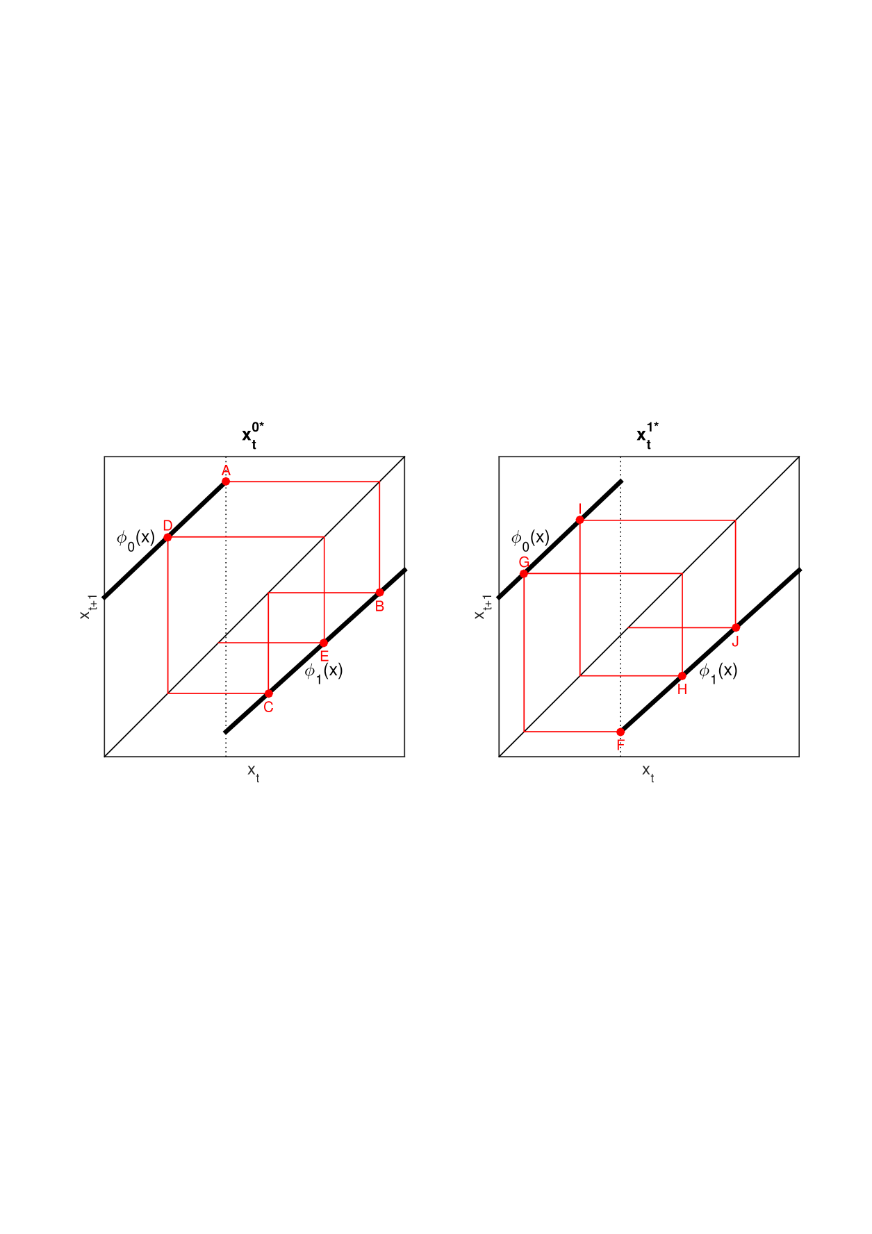
where $x_{0}^{0*}(x)=x_{0}^{1*}(x)=x$. We refer to $x_{t}^{0*}(x),x_{t}^{1*}(x)$ as the $x$-threshold orbits (Figure 1).

We are now ready to state our main result.

Theorem 1. Suppose a threshold policy (A1) is optimal for the single-arm problem (2). Then Problem KF1 is indexable. Specifically, for any $b>a\geq 0$ let

$\displaystyle\phi_{0}(x)$

$\displaystyle:=\frac{x+1}{ax+a+1},$

$\displaystyle\phi_{1}(x)$

$\displaystyle:=\frac{x+1}{bx+b+1}$

and for any $w\in\mathbb{R}_{+},h\in\mathbb{R}$ and $0<\beta<1$, let

$\displaystyle\lambda^{W}(x):=w\frac{\sum_{t=1}^{\infty}\beta^{t}(x_{t}^{0*}(x)-x_{t}^{1*}(x))}{\sum_{t=0}^{\infty}\beta^{t}(u^{1*}_{t}(x)-u^{0*}_{t}(x))}-h$

(6)

in which action sequences $u_{t}^{0*}(x),u_{t}^{1*}(x)$ and error variance sequences $x_{t}^{0*}(x),x_{t}^{1*}(x)$ are given in terms of $\phi_{0},\phi_{1}$ by (5). Then $\lambda^{W}(x)$ is a continuous and non-decreasing function of $x\in\mathbb{R}_{+}$.

We are now ready to describe the key concepts underlying this result.

Words. In this paper, a word $w$ is a string on $\{0,1\}^{*}$ with $k^{\rm th}$ letter $w_{k}$ and $w_{i:j}:=w_{i}w_{i+1}\dots w_{j}$. The empty word is $\epsilon$, the concatenation of words $u,v$ is $uv$, the word that is the $n$-fold repetition of $w$ is $w^{n}$, the infinite repetition of $w$ is $w^{\omega}$ and $\tilde{w}$ is the reverse of $w$, so $w=\tilde{w}$ means $w$ is a palindrome. The length of $w$ is ${\left|w\right|}$ and ${\left|w\right|}_{u}$ is the number of times that word $u$ appears in $w$, overlaps included.

Christoffel, Sturmian and Mechanical Words. It turns out that the action sequences in (5) are given by such words, so the following definitions are central to this paper.

The Christoffel tree (Figure 2) is an infinite complete binary tree [5] in which each node is labelled with a pair $(u,v)$ of words. The root is $(0,1)$ and the children of $(u,v)$ are $(u,uv)$ and $(uv,v)$. The Christoffel words are the words $0,1$ and the concatenations $uv$ for all $(u,v)$ in that tree. The fractions ${\left|uv\right|}_{1}/{\left|uv\right|}_{0}$ form the Stern-Brocot tree [9] which contains each positive rational number exactly once. Also, infinite paths in the Stern-Brocot tree converge to the positive irrational numbers. Analogously, Sturmian words could be thought of as infinitely-long Christoffel words.

Alternatively, among many known characterisations, the Christoffel words can be defined as the words $0,1$ and the words $0w1$ where $a:={\left|0w1\right|}_{1}/{\left|0w1\right|}$ and

$\displaystyle(01w)_{n}:=\lfloor(n+1)a\rfloor-\lfloor na\rfloor$

for any relatively prime natural numbers ${\left|0w1\right|}_{0}$ and ${\left|0w1\right|}_{1}$ and for $n=1,2,\dots,{\left|0w1\right|}$. The Sturmian words are then the infinite words $0w_{1}w_{2}\cdots$ where, for $n=1,2,\dots$ and $a\in(0,1)\backslash\mathbb{Q}$,

$\displaystyle(01w_{1}w_{2}\cdots)_{n}:=\lfloor(n+1)a\rfloor-\lfloor na\rfloor.$

We use the notation $0w1$ for Sturmian words although they are infinite.

The set of mechanical words is the union of the Christoffel and Sturmian words [13]. (Note that the mechanical words are sometimes defined in terms of infinite repetitions of the Christoffel words.)

Majorisation. As in [14], let $x,y\in\mathbb{R}^{m}$ and let $x_{(i)}$ and $y_{(i)}$ be their elements sorted in ascending order. We say $x$ is weakly supermajorised by $y$ and write $x\prec^{w}y$ if

$\displaystyle\sum_{k=1}^{j}x_{(k)}\geq\sum_{k=1}^{j}y_{(k)}\qquad\text{for all $j=1,\dots,m$.}$

If this is an equality for $j=m$ we say $x$ is majorised by $y$ and write $x\prec y$. It turns out that

	$\displaystyle x\prec y\qquad$	$\displaystyle\Leftrightarrow\qquad\sum_{k=1}^{j}x_{[k]}\leq\sum_{k=1}^{j}y_{[k]}\quad\text{for $j=1,\dots,m-1$ with equality for $j=m$}$
where $x_{[k]},y_{[k]}$ are the sequences sorted in descending order. For $x,y\in\mathbb{R}^{m}$ we have [14]
	$\displaystyle x\prec y\qquad$	$\displaystyle\Leftrightarrow\qquad\sum_{i=1}^{m}f(x_{i})\leq\sum_{i=1}^{m}f(y_{i})\quad\text{for all convex functions $f:\mathbb{R}\rightarrow\mathbb{R}$.}$

More generally, a real-valued function $\phi$ defined on a subset $\mathcal{A}$ of $\mathbb{R}^{m}$ is said to be Schur-convex on $\mathcal{A}$ if $x\prec y$ implies that $\phi(x)\leq\phi(y)$.

Möbius Transformations. Let $\mu_{A}(x)$ denote the Möbius transformation $\mu_{A}(x):=\frac{A_{11}x+A_{12}}{A_{21}x+A_{22}}$ where $A\in\mathbb{R}^{2\times 2}$. Möbius transformations such as $\phi_{0}(\cdot),\phi_{1}(\cdot)$ are closed under composition, so for any word $w$ we define $\phi_{w}(x):=\phi_{w_{{\left|w\right|}}}\circ\dots\circ\phi_{w_{2}}\circ\phi_{w_{1}}(x)$ and $\phi_{\epsilon}(x):=x.$

Intuition. Here is the intuition behind our main result.

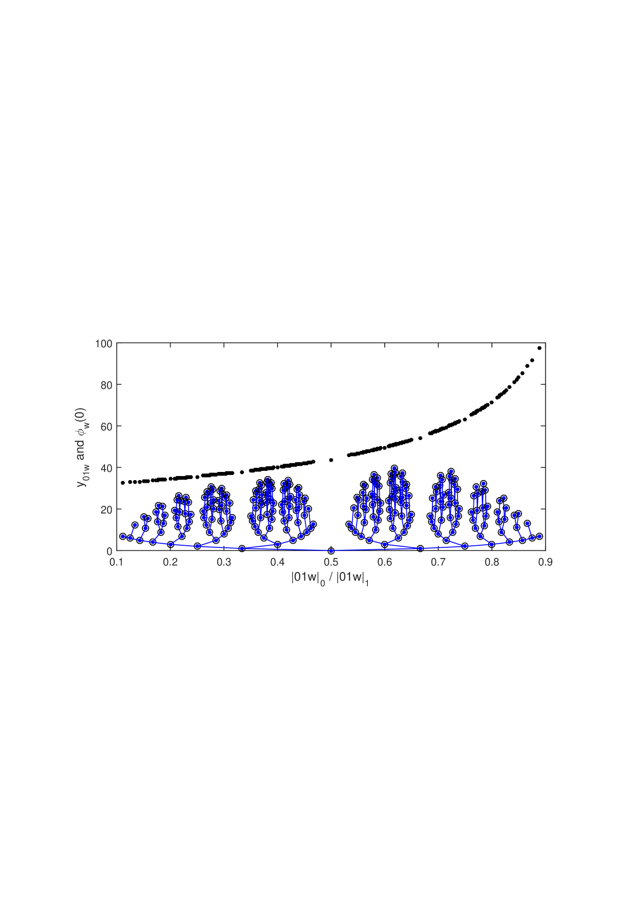
For any $x\in\mathbb{R}_{+}$, the orbits in (5) correspond to a particular mechanical word $0,1$ or $0w1$ depending on the value of $x$ (Figure 1). Specifically, for any word $u$, let $y_{u}$ be the fixed point of the mapping $\phi_{u}$ on $\mathbb{R}_{+}$ so that $\phi_{u}(y_{u})=y_{u}$ and $y_{u}\in\mathbb{R}_{+}$. Then the word corresponding to $x$ is 1 for $0\leq x\leq y_{1}$, $0w1$ for $x\in[y_{01w},y_{10w}]$ and 0 for $y_{0}\leq x<\infty$. In passing we note that these fixed points are sorted in ascending order by the ratio $\rho:={\left|01w\right|}_{0}/{\left|01w\right|}_{1}$ of counts of 0s to counts of 1s, as illustrated by Figure 3. Interestingly, it turns out that ratio $\rho$ is a piecewise-constant yet continuous function of $x$, reminiscent of the Cantor function.

Also, composition of Möbius transformations is homeomorphic to matrix multiplication so that

$\displaystyle\mu_{A}\circ\mu_{B}(x)=\mu_{AB}(x)\qquad\text{for any $A,B\in\mathbb{R}^{2\times 2}.$}$

Thus, the index (6) can be written in terms of the orbits of a linear system (11) given by $0,1$ or $0w1.$ Further, if $A\in\mathbb{R}^{2\times 2}$ and $\det(A)=1$ then the gradient of the corresponding Möbius transformation is the convex function

$\displaystyle\frac{d\mu_{A}(x)}{dx}=\frac{1}{(A_{21}x+A_{22})^{2}}.$

So the gradient of the index is the difference of the sums of a convex function of the linear-system orbits. However, such sums are Schur-convex functions and it follows that the index is increasing because one orbit weakly supermajorises the other, as we now show for the case $0w1$ (noting that the proof is easier for words $0,1$). As $0w1$ is a mechanical word, $w$ is a palindrome. Further, if $w$ is a palindrome, it turns out that the difference between the linear-system orbits increases with $x$. So, we might define the majorisation point for $w$ as the $x$ for which one orbit majorises the other. Quite remarkably, if $w$ is a palindrome then the majorisation point is $\phi_{w}(0)$ (Proposition 7). Indeed the black circles and blue dots of Figure 3 coincide. Finally, $\phi_{w}(0)$ is less than or equal to $y_{01w}$ which is the least $x$ for which the orbits correspond to the word $0w1$. Indeed, the blue dots of Figure 3 are below the corresponding black dots. Thus one orbit does indeed supermajorise the other.

References

- [1] E. Altman, B. Gaujal, and A. Hordijk. Multimodularity, convexity, and optimization properties. Mathematics of Operations Research, 25(2):324–347, 2000.
- [2] E. Altman and S. Stidham Jr. Optimality of monotonic policies for two-action Markovian decision processes, with applications to control of queues with delayed information. Queueing Systems, 21(3-4):267–291, 1995.
- [3] M. Araya, O. Buffet, V. Thomas, and F. Charpillet. A POMDP extension with belief-dependent rewards. In Neural Information Processing Systems, pages 64–72, 2010.
- [4] A. Badanidiyuru, B. Mirzasoleiman, A. Karbasi, and A. Krause. Streaming submodular maximization: Massive data summarization on the fly. In Proceedings of the 20th ACM SIGKDD International Conference on Knowledge Discovery and Data Mining, pages 671–680, 2014.
- [5] J. Berstel, A. Lauve, C. Reutenauer, and F. Saliola. Combinatorics on Words: Christoffel Words and Repetitions in Words. CRM Monograph Series, 2008.
- [6] S. Bubeck and N. Cesa-Bianchi. Regret Analysis of Stochastic and Nonstochastic Multi-armed Bandit Problems, Foundation and Trends in Machine Learning, Vol. 5. NOW, 2012.
- [7] Y. Chen, H. Shioi, C. Montesinos, L. P. Koh, S. Wich, and A. Krause. Active detection via adaptive submodularity. In Proceedings of The 31st International Conference on Machine Learning, pages 55–63, 2014.
- [8] J. Gittins, K. Glazebrook, and R. Weber. Multi-armed bandit allocation indices. John Wiley & Sons, 2011.
- [9] R. Graham, D. Knuth, and O. Patashnik. Concrete Mathematics: A Foundation for Computer Science. Addison-Wesley, 1994.
- [10] S. Guha, K. Munagala, and P. Shi. Approximation algorithms for restless bandit problems. Journal of the ACM, 58(1):3, 2010.
- [11] B. La Scala and B. Moran. Optimal target tracking with restless bandits. Digital Signal Processing, 16(5):479–487, 2006.
- [12] J. Le Ny, E. Feron, and M. Dahleh. Scheduling continuous-time Kalman filters. IEEE Trans. Automatic Control, 56(6):1381–1394, 2011.
- [13] M. Lothaire. Algebraic combinatorics on words. Cambridge University Press, 2002.
- [14] A. Marshall, I. Olkin, and B. Arnold. Inequalities: Theory of majorization and its applications. Springer Science & Business Media, 2010.
- [15] L. Meier, J. Peschon, and R. Dressler. Optimal control of measurement subsystems. IEEE Trans. Automatic Control, 12(5):528–536, 1967.
- [16] J. Niño-Mora and S. Villar. Multitarget tracking via restless bandit marginal productivity indices and Kalman filter in discrete time. In Proceedings of the 48th IEEE Conference on Decision and Control, pages 2905–2910, 2009.
- [17] R. Ortner, D. Ryabko, P. Auer, and R. Munos. Regret bounds for restless Markov bandits. In Algorithmic Learning Theory, pages 214–228. Springer, 2012.
- [18] B. Rajpathak, H. Pillai, and S. Bandyopadhyay. Analysis of stable periodic orbits in the one dimensional linear piecewise-smooth discontinuous map. Chaos, 22(3):033126, 2012.
- [19] T. Thiele. Sur la compensation de quelques erreurs quasi-systématiques par la méthode des moindres carrés. CA Reitzel, 1880.
- [20] I. Verloop. Asymptotic optimal control of multi-clss restless bandits. CNRS Technical Report, hal-00743781, 2014.
- [21] S. Villar. Restless bandit index policies for dynamic sensor scheduling optimization. PhD thesis, Statistics Department, Universidad Carlos III de Madrid, 2012.
- [22] E. Vul, G. Alvarez, J. B. Tenenbaum, and M. J. Black. Explaining human multiple object tracking as resource-constrained approximate inference in a dynamic probabilistic model. In Neural Information Processing Systems, pages 1955–1963, 2009.
- [23] R. R. Weber and G. Weiss. On an index policy for restless bandits. Journal of Applied Probability, pages 637–648, 1990.
- [24] P. Whittle. Restless bandits: Activity allocation in a changing world. Journal of Applied Probability, pages 287–298, 1988.
6 Supplementary Material: Introduction
The results used but not proved in the main paper are given here as:
-
•
Proposition 9 which was used to show that ,
Proposition 16 for the range of giving a specific mechanical word,
Proposition 17 showing the index is continuous for
Proposition 19 showing the properties of when is a palindrome.
and Proposition 20 for weak supermajorisation with .
A clarification of the extreme cases of Theorem 1 of the main paper is presented in the final section.
7 From -Threshold Policies to Mechanical Words
Some concepts relating to mechanical words appeared as early as 1771 in Jean Bernoulli’s study of continued fractions (Berstel et al, 2008). The term “mechanical sequences” appears in the work of Morse and Hedlund (Am. J. Math., Vol 62, No. 1, 1940, p. 1-42) who had just introduced the term “symbolic dynamics”. Morse and Hedlund studied the concept from the perspective of sequences of the form for and . They also studied the concept from the perspective of differential equations, motivating the term “Sturmian sequences.” Since that time there has been tremendous progress in the study of such sequences from the perspective of Combinatorics on Words (Lothaire, 2001). However, the recent (and highly-approachable) paper of Rajpathak, Pillai and Bandyopadhyay (Chaos, Vol. 22, 2012) on the piecewise-linear map-with-a-gap discovers such sequences without recognising them as mechanical sequences. Proposition 16 of this section is a substantial generalisation of that result and we could not find this proposition explicitly stated in the literature. Our result is not surprising if one has the intuition that there is a topological conjugacy between the maps of this section and the piecewise linear map-with-a-gap. However, it might be difficult to explicitly identify the appropriate topological conjugacy and thereby prove our result for all cases considered here.
7.1 Definitions
Let denote a word consisting of a string of 0s and 1s in which the letter is and letters are . Let be the length of and for a word be the number of times that word appears in . Let denote the empty word and denote the infinite word constructed by repeatedly concatenating .
Consider two functions and where is an interval of We define the transformation for any word by the composition
Let be the fixed point of , so , assuming a unique fixed point on exists.
Given , we call the sequence the -threshold orbit for if
We call the -threshold word for if it is the shortest word such that for all . We shall just write -threshold orbit and -threshold word where are obvious from the context.
For , let be the morphisms (substitutions)
We say is a valid word if or for some valid word .
Remark. The morphisms generate the Christoffel tree so valid words are mechanical words. To see this, note that the Christoffel tree is generated by the following morphisms (Berstel et al, 2008, p. 37)
We may translate (from English to French) as and so any composition of and can be written as a composition of and . Likewise, any composition of and can be written as a composition of and . Specifically if then
whereas if we have
A symmetric argument holds if or .
7.2 Fixed Points
Throughout, we make the following assumption about . The existence of fixed points is addressed immediately thereafter.
Assumption A2. Functions , where is an interval of , are increasing and non-expansive. Equivalently, for all and for we have
Furthermore, the fixed points of satisfy .
Proposition 8.
Suppose A2 holds, that and that is any non-empty word. Then is increasing and non-expansive. Further, the fixed point exists and is unique.
Proof.
First we show that is increasing, by induction. In the base case, and the claim follows from A2. For the inductive step assume is increasing, where for some and word . Then for any ,