Whole-Word Segmental Speech Recognition with Acoustic Word Embeddings
Abstract
Segmental models are sequence prediction models in which scores of hypotheses are based on entire variable-length segments of frames. We consider segmental models for whole-word (“acoustic-to-word”) speech recognition, with the feature vectors defined using vector embeddings of segments. Such models are computationally challenging as the number of paths is proportional to the vocabulary size, which can be orders of magnitude larger than when using subword units like phones. We describe an efficient approach for end-to-end whole-word segmental models, with forward-backward and Viterbi decoding performed on a GPU and a simple segment scoring function that reduces space complexity. In addition, we investigate the use of pre-training via jointly trained acoustic word embeddings (AWEs) and acoustically grounded word embeddings (AGWEs) of written word labels. We find that word error rate can be reduced by a large margin by pre-training the acoustic segment representation with AWEs, and additional (smaller) gains can be obtained by pre-training the word prediction layer with AGWEs. Our final models improve over prior A2W models.
Index Terms— speech recognition, segmental model, acoustic-to-word, acoustic word embeddings, pre-training
1 Introduction
Acoustic-to-word (A2W) models for speech recognition map input acoustic frames directly to words. Unlike conventional subword-based automatic speech recognition (ASR) systems, A2W models do not require an external lexicon, thus simplifying training and decoding. Recent work has shown that A2W models can achieve performance competitive with state-of-the-art subword-based systems either with large amounts of training data [1] or with careful training techniques [2, 3, 4, 5].
Most work on A2W models [1, 2, 3, 6, 4, 5, 7] is based on connectionist temporal classification (CTC) [8], where the word sequence probability is defined as the product of frame-level probabilities. In such approaches there is no explicit modeling of segments of frames corresponding to words. There has also been recent work on encoder-decoder A2W models, which can focus on ”soft segments” via an attention mechanism [9, 10].
In this paper we propose an approach using whole-word segmental models, where the sequence probability is computed based on segment scores instead of frame probabilities. Segmental models have a long history in speech recognition research, but they have been used primarily for phonetic recognition or as phone-level acoustic models [11, 12, 13, 14, 15, 16, 17, 18]. There has also been work on whole-word segmental models for second-pass rescoring [13, 19, 20], but to our knowledge our approach is the first to address end-to-end A2W segmental models.
The key ingredient in our approach is to define the segment scores in terms of dot products between vector embeddings of acoustic segments and a weight layer of written word embeddings. This form of the model allows for (1) efficient re-use of feature functions and therefore reduced memory cost and (2) initialization of the acoustic and written embeddings using pre-trained acoustic word embeddings (AWEs) and acoustically grounded word embeddings (AGWEs), following the successful use of such pre-training in prior work on speech recognition [5] and search [21, 22]. We also obtain speed-ups via GPU implementations of the forward-backward and Viterbi algorithms. We find that pre-trained AWEs provide large gains, and result in segmental models that outperform the best prior A2W models on conversational telephone speech recognition.
2 Segmental Model Formulation
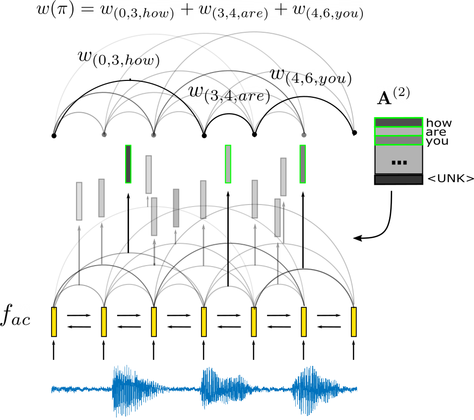
Segmental models compute the score of a hypothesized label sequence as a combination of scores of multi-frame segments of speech in the sequence, rather than using individual frame scores (see Figure 1). Let be a sequence of input acoustic frames and be the output label sequence. A segmentation with respect to and is defined as a sequence of tuples . Each tuple defines a segment consisting of a start timestep111Frame is the acoustic signal between timesteps and . , an end timestep , and a label , such that and for all . A segmental model assigns a score to each segment . The score of a segmentation is then defined as .
2.1 Segment Score Functions
As in other recent sequence models, the input acoustic frames are first passed through a neural network and encoded into frame features , where denotes the feature dimensionality. In segmental models, however, these frame features are then used to produce segment scores , where and denote the maximum segment size and vocabulary size, respectively, and is the score of segment . Our approach defines segment scores in terms of dot products between learned representations of variable-length segments and word labels:
| (1) |
where is an acoustic segment embedding function mapping segments to fixed-dimensional embeddings , is a row from the matrix composed of embeddings for all words in the vocabulary, and is the bias on word , which can be interpreted as a log-unigram probability. We define the acoustic segment embedding function as follows:
| (2) |
where is a pooling function chosen between:
| (3) | |||
| (4) | |||
| (5) |
where (3) is concatenation, (4) is mean pooling, and (5) is attention pooling (with learnable parameter g). Equation 1 allows feature sharing, which helps limit the memory needed to compute segment features to and simplifies scoring to matrix multiplication, i.e. .
Recent work on segmental models has largely used two types of segment score functions: (1) frame classifier-based [16, 23, 15, 24] and (2) segmental recurrent neural network (SRNN) [18, 25, 24]. Frame classifier-based score functions use a mapping from input acoustic frames to frame log-probability vectors , which are then pooled (via mean, sampling, etc.) to get the segment score . This method introduces a multiplicative memory dependence on , which is a factor increase in memory overhead over our approach. In our case is the number of words in the vocabulary, which is typically times larger than and makes this approach extremely (sometimes prohibitively) expensive. SRNNs compute the score , where is a learned feature function, is an embedding of word , and denotes concatenation of . This method introduces an memory overhead, which can again quickly make it infeasible for large-vocabulary recognition.
2.2 Training
Segmental models can be trained in a variety of ways [24]. One way, which we adopt here, is to interpret them as probabilistic models and optimize the marginal log loss under that model, which is equivalent to viewing our models as segmental conditional random fields [27]. Under this view, the model assigns probabilities to paths, conditioned on the input acoustic sequence, by normalizing the path score. Letting , we define as the probability of the segmentation, where and denotes all segmentations of . We define the loss for a given word sequence and input as the marginal log loss, by marginalizing over all possible segmentations:
| (6) |
where maps to its label sequence . The summations can be efficiently computed with dynamic programming:
| (7) |
With and computed, the loss value follows directly from . The last summations in Equations 7 can be efficiently implemented on a GPU. In addition, can be computed in parallel given such that the overall time complexity222Number of times is called of computing the loss is .
To train with gradient descent, we need to differentiate with respect to , which can in principle be done with auto-differentiation toolkits (e.g. PyTorch [28]). However, in practice using auto-differentiation to compute the gradient is many times slower than the loss computation. Instead we explicitly implement the gradient computation using the backward algorithm. We define two backward variables and for the denominator and numerator, respectively:
| (8) |
The gradient is then given by
| (9) |
where are the indices in where label occurs.
2.3 Decoding
Decoding consists of solving . This optimization problem can be solved efficiently via the Viterbi algorithm with the recursive relationship:
| (10) |
where the last max operation can be parallelized on a GPU such that the overall runtime333Number of times is called of decoding is only .
2.4 Pre-training via acoustic and acoustically grounded word embeddings
One important issue in whole-word models is that many words are infrequent or unseen in the training set. In particular, the final weight layer, which corresponds to embeddings of the word labels, can be very poorly learned. Recent work has shown that jointly pre-trained acoustic word embeddings (AWEs) and corresponding acoustically grounded word embeddings (AGWEs) of the written words [26] can serve as a good parameter initialization for CTC-based A2W models [5], improving conversational speech recognition performance. In this prior work, the AGWEs are parametric functions of character sequences, so that word embeddings can be produced for unseen or infrequent words. We follow this idea and jointly pre-train our segmental acoustic embedding function and the corresponding weight layer in Equation 1. This initialization is especially natural for whole-word segmental models, since the segments are explicitly intended to model words. Note that typical pre-trained written word embeddings (such as word2vec [29], GloVe [30], and contextual word embeddings [31, 32]) are not what is needed for the label embedding layer; we are interested in embeddings that represent the way a word sounds rather than what it means, so acoustically grounded embeddings are the more natural choice.
Our pre-training follows the multi-view AWE+AGWE training approach of [26, 5], in which we jointly train an acoustic “view” embedding model () and a written “view” model () using a contrastive loss. The written view model takes in a word label , maps to a subword (e.g., character/phone) sequence using a lexicon, and uses this sequence to produce an embedding vector as output. The resulting written word embedding model is ”acoustically grounded” because it is learned jointly with the acoustic embedding model so as to represent the way the word sounds. Specifically, we use an objective consisting of three contrastive triplet loss terms:
| (11) |
where is a spoken word segment, is its word label, is a margin hyperparameter, denotes cosine distance , and is the number of training pairs . We conduct semi-hard [33] negative sampling w.r.t. each pair:
where is the training vocabulary and is the word label of . For efficiency, this negative sampling is performed over the mini-batch such that is the batch size and consists of words in the mini-batch. Additionally, rather than the single most offending semi-hard negative we use and each contrastive loss term inside the sum in Equation 11 is an average over these negatives. The contrastive loss aims to map spoken word segments corresponding to the same word label close together and close to their learned label embeddings, while ensuring that segments corresponding to different word labels are mapped farther apart (and nearer to their respective label embeddings). Our pre-training approach is the same as that of [26, 5] except for the addition of semi-hard negative sampling (replacing hard negative sampling in [5]), the inclusion of a third contrastive term ( of [26]), and an extra convolutional layer and pooling in the AWE encoder (see Section 3). The first two changes increase word discrimination task performance in prior work on AWEs [34, 35, 26], and the third change improves efficiency of the segmental model.
The pre-trained AWE/AGWE models are tuned using a cross-view word discrimination task as in [26, 5], applied to word segments from the development set and word labels from the vocabulary. The task is to determine whether a given acoustic word segment and word label match. We compute the embeddings of the acoustic segment and character sequence by forwarding them through and , respectively, and then compute their cosine distance. If this distance is below a threshold, then the pair is labeled a match. The quality of the embeddings is measured by the average precision (AP) over all thresholds over the dev set.
3 Experiments
We conduct experiments on the standard Switchboard-300h dataset and data division [36]. We use 40-dimensional log-Mel spectra ++s, extracted with Kaldi [37], as input features. Every two successive frames are stacked and alternate frames dropped, resulting in 240-dimensional features. We explore , , and vocabularies based on word occurrence thresholds of , , and , respectively. Hyperparameters are chosen based on prior related work (e.g., [5]) and light tuning on the Switchboard development set. The backbone network for the segmental model is a 6-layer bidirectional long short-term memory network (BiLSTM) with 512 hidden units per direction per layer with dropout added between layers (0.25 except when otherwise specified below). To speed up training, we add a convolutional layer with kernel size 5 followed by average pooling with stride 4 on top of the BiLSTM. The maximum segment length is set to 32, corresponding to a maximum word duration of . To further speed up training, we reduce the maximum segment size per batch (batch size: 16) to . The model is trained with the Adam optimizer [38] with an initial learning rate of 0.001, which is decreased by a factor of 2 when the dev WER stops decreasing. No language model is used for decoding. As a baseline, we also train an A2W CTC model using the same structure (6-layer BiLSTM + convolutional + pooling).
3.1 Phone CTC pre-training
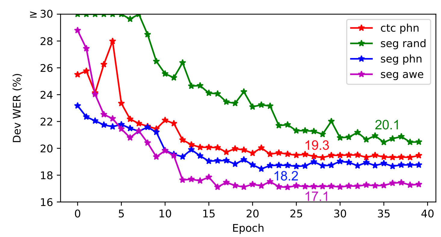
As an initial experiment with the 5K vocabulary, we initialize the backbone BiLSTM network by pre-training with a phone CTC objective, as in prior work on CTC-based A2W models [2, 3, 4, 5]. The phone error rate (PER) of this phone CTC model is . On top of the pre-trained BiLSTM, the convolutional layer and word embedding parameters () in our segmental model are randomly initialized. Compared to random initialization, phone CTC pre-training reduces WER by (Figure 2), which is consistent with prior work [2]. When both our segmental model and the baseline A2W CTC model are pre-trained with phone CTC, our model achieves lower word error rate (WER) (Figure 2).
The pooling operation in Equation 2 is tuned among mean pooling (18.5%), attention pooling (19.0%) and concatenation (18.2%). The best performance is obtained with concatenation, which also increases the feature dimensionality of , while consuming a factor of less memory when computing segment features.
| System | Vocab size | ||
|---|---|---|---|
| 5K | 10K | 20K | |
| A2W CTC with phone CTC init | 19.3 | 18.0 | 17.7 |
| A2W Segmental with phone CTC init | 18.2 | 17.9 | 18.0 |
| + AGWE init | 18.4 | 18.0 | 18.0 |
| A2W Segmental with AWE init | 17.1 | 16.0 | 16.4 |
| + AGWE init | 17.1 | 15.8 | 16.5 |
| + AGWE reg | 17.0 | 15.5 | 15.6 |
3.2 Vocabulary size
We find that, unlike our A2W CTC models and those of prior work [5, 4], the segmental models do not necessarily improve with larger vocabulary. One possible reason is that word representations in segmental models, especially for rare words, are harder to learn as they must be robust to variations in segment duration and content. Segmental models may require more data when many rare words are included. We find that it is important to set a larger dropout value as the vocabulary size increases. The best dropout values for , and are , , and , respectively, with results in Table 1.
3.3 AWE + AGWE pre-training
We now investigate whether pre-training with AWE and AGWEs can provide a better starting point for the segmental model. We jointly train AWE and AGWE models on the Switchboard-300h training set with the multi-view training approach described in Section 2.4. Early stopping and hyperparameter tuning are done based on the cross-view average precision (AP) on the same development set as in ASR training. In the contrastive training objective, we use , reduced by per batch until , and a variable batch size with up to frames per batch. The acoustic view model has the same structure as in the segmental model, and the written view model is composed of an input embedding layer mapping input characters to -dimensional embeddings followed by a 1-layer BiLSTM with 256 hidden units per direction. We optimize with the Adam optimizer [38], with an initial learning rate of 0.0005, which is reduced by a factor of 10 when the development set cross-view AP does not improve for steps. Training is stopped when the learning rate drops below . After multi-view training, the acoustic view (our AWE function) and the written view (our AGWE function) are used to initialize our segmental feature function and , respectively, in Equation 1.
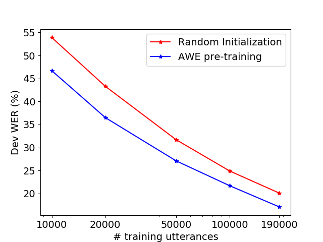
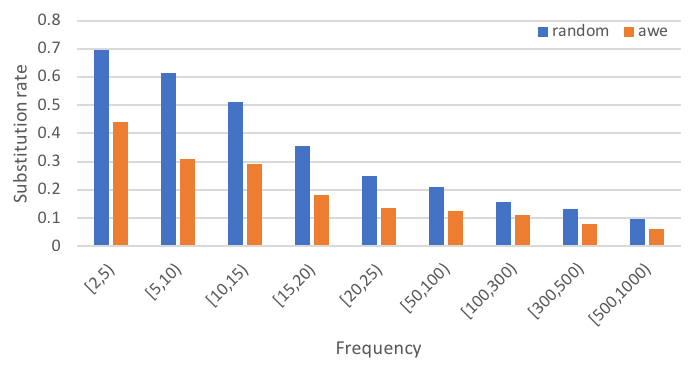
Table 1 compares an A2W CTC model with segmental models using different initializations, evaluated on the SWB development set. Initialization of with the pre-trained AWE model reduces WER by – over phone CTC initialization. Initialization of with pre-trained AGWE models alone does not help, but initializing with AWE and AGWE while regularizing toward the pre-trained AGWEs (see Section 2.4) is helpful, especially for larger vocabularies. This observation is consistent with our expectation: Since the AGWEs are composed from character sequences, they are less impacted by vocabulary size, helping with recognition of rare words. We also note that the optimal in Equation 12 tends to be larger as the vocabulary size increases, reinforcing the need for more regularization when there are many rare words. This intuition about rare words also suggests that AWE pre-training should be more helpful for smaller training sets and for rarer words. Figures 3 and 4 demonstrate this expected result.
3.4 Final evaluation results
Table 2 shows the final results on the Switchboard (SWB) and CallHome (CH) test sets, compared to prior work with A2W models.444We do not compare with prior segmental models [17, 18] since, due to their larger memory footprint, we are unable to train them for A2W recognition with a similar network architecture using a typical GPU (e.g., 12GB memory). For the smaller vocabularies (, ), the segmental model improves WER over CTC by around (absolute). Training with SpecAugment [39] produces an additional gain of across all vocabulary sizes. As noted before, the -word model outperforms the -word one. In addition to the issue of rare words, the longer training time with a -word vocabulary prevents us from tuning hyperparamters as much as for the models. Overall our best model improves over all previous A2W models of which we are aware, although our model is smaller than the previous best-performing model [4].
Despite the improved performance of our A2W models, there is still a gap between our (and all) A2W models and systems based on subword units, where the best performance on this task of which we are aware is 6.3% on SWB and 13.3% on CH using a sub-word based sequence-to-sequence transformer model [39]. Some prior work suggests that the gap between between A2W and subword-based models can be significantly narrowed when using larger training sets, and our future work includes investigations with larger data. At the same time, A2W models retain the benefit of being very simple, truly end-to-end models that avoid using a decoder or potentially a language model.
| System | Vocab | ||
|---|---|---|---|
| 4K/5K | 10K | 20K | |
| Seg, AWE+AGWE init | 14.0/24.9 | 12.8/23.5 | 12.5/24.5 |
| +SpecAugment | 12.8/22.9 | 10.9/20.3 | 12.0/21.9 |
| CTC, phone init [5] | 16.4/25.7 | 14.8/24.9 | 14.7/24.3 |
| CTC, AWE+AGWE init [5] | 15.6/25.3 | 14.2/24.2 | 13.8/24.0 |
| +reg[5] | 15.5/25.4 | 14.0/24.5 | 13.7/23.8 |
| CTC, AWE+AGWE rescore [5] | 15.0/25.3 | 14.4/24.5 | 14.2/24.7 |
| S2S [10] | - | 22.4/36.1 | 22.4/36.2 |
| Curriculum [4] | - | - | 13.4/24.2 |
| +Joint CTC/CE[4] | - | - | 13.0/23.4 |
| +Speed Perturbation[4] | - | - | 11.4/20.8 |
3.5 Decoding and training speed
| Model | training | decoding, GPU | decoding, CPU |
|---|---|---|---|
| CTC | 368.2 (40.3) | 61.0 (0.6) | 634.5 (0.6) |
| Seg, ours | 509.6 (69.1) | 92.9 (32.7) | 1009.8 (60.1) |
| Seg, SRNN | 1739.7 (72.8) | 120.9 (35.4) | 1232.5 (57.4) |
| Seg, FC | 1361.5 (71.5) | 109.7 (33.2) | 1031.4 (60.4) |
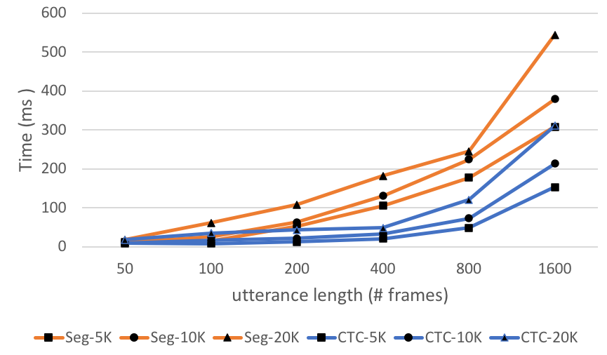
Our implementation is based on PyTorch, with the forward/backward computation for the segmental loss implemented in CUDA C. Training on the 300-hour Switchboard training set takes about 2 days on one Titan X GPU. Figure 5 shows the latency of the loss forward/backward computation compared with CTC. For CTC we use the Warp-CTC implementation in ESPnet [40]. The segmental loss forward/backward computation is roughly x slower than for CTC, which is mainly due to the denominator computations ( and in Equations 7, 8). We also measure training time per batch and decoding time per utterance averaged over 100 random batches from the dev set (see Table 3).
To demonstrate the efficiency improvement enabled by our segmental feature function, we also compare to (our implementation of) a whole-word SRNN [18] and a whole-word frame classifier (FC)-based segmental model [24] with the same backbone network. The SRNN/FC-based models differ from our segmental model in terms of the feature functions, but we use the same implementation of the forward/backward/Viterbi algorithms for all three models. We note that, in order to make the speed comparison with an FC-based model possible, we simplified it somewhat so as to fit it into GPU memory.555Specifically, we removed the frame average feature function (Equation 6 in [24]) and added an extra linear layer on top of the BiLSTM to reduce dimensionality of and to 1 (first equation in Section III.B in [24]). These two models are implemented only for this speed test; we fail to train them to completion because, even with our simplifications, we still run out of memory for some training utterances. Overall our segmental model is roughly x slower to train than CTC but more than twice faster than the SRNN/FC-based models. In practice, the loss computation is a small fraction of the total training time (see Table 3). Computing the segment score function is the main factor that accounts for the larger training latency compared to CTC.
Similarly, our segmental model is also x slower than CTC in decoding. Compared to CTC, the actual decoding algorithm accounts for a larger proportion of the total latency. The CTC greedy decoding can be parallelized more () than Viterbi decoding (). However, using a GPU results in larger speed gains for Viterbi decoding.
4 Conclusion
We have introduced an end-to-end whole-word segmental model, which to our knowledge is the first to perform large-vocabulary speech recognition competitively and efficiently. Our model uses a simple segment score function based on a dot product between written word embeddings and acoustic segment embeddings, which both improves efficiency and enables us to pre-train the model with jointly trained acoustic and written word embeddings. We find that the proposed model outperforms previous A2W approaches, and is much more efficient than previous segmental models. The key aspects that are important to the performance improvements are pre-training the acoustic segment representation with acoustic word embeddings and regularizing the label embeddings toward pre-trained acoustically grounded word embeddings. Given the good performance of segmental models especially when the label set is relatively small, it will also be interesting to apply the approach to recognition based on subwords like byte pair encodings [41] or other more acoustically motivated subwords [42], and to study the applicability of our models to a wider range of training set sizes and domains.
5 Acknowledgements
We are grateful to Hao Tang for helpful suggestions and discussions. This research was funded by NSF award IIS-1816627, and by an AWS Machine Learning Research Award.
References
- [1] H. Soltau, H. Liao, and H. Sak, “Neural speech recognizer: Acoustic-to-word LSTM model for large vocabulary speech recognition,” in Proc. Interspeech, 2016.
- [2] K. Audhkhasi, B. Ramabhadran, G. Saon, M. Picheny, and D. Nahamoo, “Direct acoustics-to-word models for English conversational speech recognition,” in Proc. Interspeech, 2017.
- [3] Kartik Audhkhasi, Brian Kingsbury, Bhuvana Ramabhadran, George Saon, and Michael Picheny, “Building competitive direct acoustics-to-word models for English conversational speech recognition,” in Proc. Interspeech, 2018.
- [4] Chengzhu Yu, Chunlei Zhang, Chao Weng, Jia Cui, and Dong Yu, “A multistage training framework for acoustic-to-word model,” in Proc. Interspeech, 2018.
- [5] Shane Settle, Kartik Audhkhasi, Karen Livescu, and Michael Picheny, “Acoustically grounded word embeddings for improved acoustics-to-word speech recognition,” in Proc. ICASSP, 2019.
- [6] Jinyu Li, Guoli Ye, Amit Das, Rui Zhao, and Yifan Gong, “Advancing acoustic-to-word CTC model,” in Proc. ICASSP, 2018.
- [7] Yashesh Gaur, Jinyu Li, Zhong Meng, and Yifan Gong, “Acoustic-to-phrase models for speech recognition,” in Proc. Interspeech, 2019.
- [8] Alex Graves, Santiago Fernández, Faustino Gomez, and Jürgen Schmidhuber, “Connectionist temporal classification: labelling unsegmented sequence data with recurrent neural networks,” in Proc. Int. Conf. on Machine Learning (ICML), 2006.
- [9] Ronan Collobert, Awni Hannun, and Gabriel Synnaeve, “Word-level speech recognition with a dynamic lexicon,” arXiv preprint arXiv:1906.04323, 2019.
- [10] Shruti Palaskar and Florian Metze, “Acoustic-to-word recognition with sequence-to-sequence models,” in Proc. IEEE Workshop on Spoken Language Technology (SLT), 2018.
- [11] Mari Ostendorf, Vassilios Digalakis, and Owen Kimball, “From HMM’s to segment models: a unified view of stochastic modeling for speech recognition,” IEEE Trans. Speech and Audio Processing, vol. 4, pp. 360–378, 1996.
- [12] James R Glass, “A probabilistic framework for segment-based speech recognition,” Computer Speech & Language, vol. 17, no. 2-3, pp. 137–152, 2003.
- [13] Geoffrey Zweig and Patrick Nguyen, “A segmental CRF approach to large vocabulary continuous speech recognition,” in Proc. IEEE Workshop on Automatic Speech Recognition and Understanding (ASRU), 2009.
- [14] Geoffrey Zweig, “Classification and recognition with direct segment models,” Proc. ICASSP, pp. 4161–4164, 2012.
- [15] Yanzhang He and Eric Fosler-Lussier, “Efficient segmental conditional random fields for phone recognition,” in Proc. Interspeech, 2012.
- [16] O. Abdel-Hamid, L. Deng, D. Yu, and H. Jiang, “Deep segmental neural networks for speech recognition,” in Proc. Interspeech, 2013.
- [17] Hao Tang, Kevin Gimpel, and Karen Livescu, “A comparison of training approaches for discriminative segmental models,” in Proc. Interspeech, 2014.
- [18] Liang Lu, Lingpeng Kong, Chris Dyer, Noah A. Smith, and Steve Renals, “Segmental recurrent neural networks for end-to-end speech recognition,” in Proc. Interspeech, 2016.
- [19] Andrew L Maas, Stephen D Miller, Tyler M O’neil, Andrew Y Ng, and Patrick Nguyen, “Word-level acoustic modeling with convolutional vector regression,” in Proc. ICML Workshop on Representation Learning, 2012.
- [20] Samy Bengio and Georg Heigold, “Word embeddings for speech recognition,” in Proc. ICASSP, 2014.
- [21] Shane Settle, Keith Levin, Herman Kamper, and Karen Livescu, “Query-by-example search with discriminative neural acoustic word embeddings,” in Proc. Interspeech, 2017.
- [22] Kartik Audhkhasi, Andrew Rosenberg, Abhinav Sethy, Bhuvana Ramabhadran, and Brian Kingsbury, “End-to-end ASR-free keyword search from speech,” IEEE Journal of Selected Topics in Signal Processing, vol. 11, no. 8, pp. 1351––1359, 2017.
- [23] Hao Tang, Weiran Wang, Kevin Gimpel, and Karen Livescu, “Discriminative segmental cascades for feature-rich phone recognition,” in Proc. IEEE Workshop on Automatic Speech Recognition and Understanding (ASRU), 2015.
- [24] Hao Tang, Liang Lu, Kevin Gimpel, Chris Dyer, and Ann S. Smith, “End-to-end neural segmental models for speech recognition,” IEEE Journal of Selected Topics in Signal Processing, 2017.
- [25] Lingpeng Kong, Chris Dyer, and Noah A. Smith, “Segmental recurrent neural networks,” in Proc. Int. Conf. on Learning Representations (ICLR), 2016.
- [26] W. He, W. Wang, and K. Livescu, “Multi-view recurrent neural acoustic word embeddings,” in Proc. Int. Conf. on Learning Representations (ICLR), 2017.
- [27] Geoffrey Zweig et al., “Speech recognition with segmental conditional random fields: A summary of the JHU CLSP 2010 summer workshop,” in Proc. ICASSP, 2011.
- [28] Adam Paszke et al., “PyTorch: An imperative style, high-performance deep learning library,” in Advances in Neural Information Processing Systems (NIPS), 2019.
- [29] Tomas Mikolov, Kai Chen, Gregory S. Corrado, and Jeffrey Dean, “Efficient estimation of word representations in vector space,” CoRR, vol. abs/1301.3781, 2013.
- [30] J. Pennington, R. Socher, and C. Manning, “GloVe: Global vectors for word representation,” in Proc. Conf. on Empirical Methods in Natural Language Processing (EMNLP), 2014.
- [31] Matthew E. Peters, Mark Neumann, Mohit Iyyer, Matt Gardner, Christopher Clark, Kenton Lee, and Luke Zettlemoyer, “Deep contextualized word representations,” in Proc. NAACL, 2018.
- [32] Jacob Devlin, Ming-Wei Chang, Kenton Lee, and Kristina Toutanova, “BERT: Pre-training of deep bidirectional transformers for language understanding,” in Proc. NAACL, 2019.
- [33] F. Schroff, D. Kalenichenko, and J. Philbin, “FaceNet: A unified embedding for face recognition and clustering,” in Proc. IEEE Conf. Computer Vision and Pattern Recognition (CVPR), 2015.
- [34] S. Settle and K. Livescu, “Discriminative acoustic word embeddings: Recurrent neural network-based approaches,” in Proc. IEEE Workshop on Spoken Language Technology (SLT), 2016.
- [35] H. Kamper, W. Wang, and K. Livescu, “Deep convolutional acoustic word embeddings using word-pair side information,” in Proc. ICASSP, 2016.
- [36] John J Godfrey, Edward C Holliman, and Jane McDaniel, “SWITCHBOARD: Telephone speech corpus for research and development,” in Proc. ICASSP, 1992.
- [37] Daniel Povey, Arnab Ghoshal, Gilles Boulianne, Lukas Burget, Ondrej Glembek, Nagendra Goel, Mirko Hannemann, Petr Motlicek, Yanmin Qian, Petr Schwarz, et al., “The Kaldi speech recognition toolkit,” in Proc. IEEE Workshop on Automatic Speech Recognition and Understanding (ASRU), 2011.
- [38] Diederik Kingma and Jimmy Ba, “Adam: A method for stochastic optimization,” in Proc. Int. Conf. on Learning Representations (ICLR), 2014.
- [39] Daniel S. Park, William Chan, Yu Zhang, Chung-Cheng Chiu, Barret Zoph, Ekin D. Cubuk, and Quoc V. Le, “SpecAugment: A simple data augmentation method for automatic speech recognition,” in Proc. Interspeech, 2019.
- [40] Shinji Watanabe et al., “ESPnet: End-to-end speech processing toolkit,” in Proc. Interspeech, 2018.
- [41] Rico Sennrich, Barry Haddow, and Alexandra Birch, “Neural machine translation of rare words with subword units,” in Proc. Association for Computational Linguistics, 2016.
- [42] Hainan Xu, Shuoyang Ding, and Shinji Watanabe, “Improving end-to-end speech recognition with pronunciation-assisted sub-word modeling,” in Proc. ICASSP, 2019.