Why do we regularise in every iteration
for imaging inverse problems?
Abstract
Regularisation is commonly used in iterative methods for solving imaging inverse problems.
Many algorithms involve the evaluation of the proximal operator of the regularisation term in every iteration, leading to a significant computational overhead
since such evaluation can be costly.
In this context, the ProxSkip algorithm, recently proposed for federated learning purposes,
emerges as an solution. It randomly skips regularisation steps, reducing the computational time of an iterative algorithm without affecting its convergence.
Here we explore for the first time the efficacy of ProxSkip to a variety of imaging inverse problems and we also propose a novel PDHGSkip version. Extensive numerical results highlight the potential of these methods to accelerate computations while maintaining high-quality reconstructions.
Keywords— Inverse problems, Iterative regularisation, Proximal operator, Stochastic optimimisation.
1 Introduction
Inverse problems involve the process of estimating an unknown quantity from indirect and often noisy measurements obeying . Here denote finite dimensional spaces, is a linear forward operator, is the ground truth and is a random noise component. Given and , the goal is to compute an approximation of . Since inverse problems are typically ill-posed, prior information about has to be incorporated in the form of regularisation. The solution to the inverse problem is then acquired by solving
| (1) |
Here denotes the fidelity term, measuring the distance between and the solution under the operator . Regularisation term promotes properties such as smoothness, sparsity, edge preservation, and low-rankness of the solution, and is weighted by a parameter . Classical examples for in imaging include the well-known Total Variation (TV), high order extensions [1], namely the Total Generalized Variation (TGV) [2], Total Nuclear Variation [3] and more general tensor based structure regularisation, [4].
In order to obtain a solution for (1), one employs iterative algorithms such as Gradient Descent (GD) for smooth objectives or Forward-Backward Splitting (FBS) [5] for non-smooth ones. Moreover, under the general framework
| (2) |
the Proximal Gradient Descent (PGD) algorithm, also known as Iterative Shrinkage Thresholding Algorithm (ISTA) and its accelerated version FISTA [6] are commonly used when is a convex, L-smooth and proper convex. Saddle-point methods such as the Primal Dual Hybrid Gradient (PDHG) [7] are commonly used for non-smooth .
A common property of most of these methods, see Algorithms 1–3 below, is the evaluation of proximal operators related to the regulariser in every iteration, which for is defined as
| (3) |
This proximal operator can have either a closed form solution, e.g., when or requires an inner iterative solver e.g., when .
The ProxSkip algorithm
The possibility to skip the computation of the proximal operator in some iterations according to a probability , accelerating the algorithms, without affecting convergence, was discussed in[8]. There, the ProxSkip algorithm was introduced to tackle federated learning applications which also rely on computations of expensive proximal operators. ProxSkip introduces a control variable , see Algorithm 4. When the proximal step is not applied, the control variable remains constant. Hence, if at iteration , no proximal step has been applied previously, the accumulated error is passed to without incurring an additional computational cost. If at the iteration the proximal step is applied, the error is reduced and the control variable will be updated accordingly.
In [8] it was shown that the ProxSkip converges provided that in (2) is L-smooth and -strongly convex, and probability satisfies
| (4) |
In the case of equality in (4), the algorithm converges (in expectation) at a linear rate with and the iteration complexity is . In addition, the total number of proximal evaluations (in expectation) are only .
Our contribution
Our aim is to showcase for the first time via extended numerical experiments the computational benefits of ProxSkip for a variety of imaging inverse problems, including challenging real-world tomographic applications. In particular, we show that ProxSkip can outperform the accelerated version of its non-skip analogue, namely FISTA. At the same time, we introduce a novel PDHGSkip version of the PDHG, Algorithm 6, which we motivate via numerical experiments. We anticipate that this will spark further research around developing skip-versions of a variety of proximal based algorithms used nowadays.
For all our imaging experiments we consider the following optimisation problem that contains a quadratic distance term as the fidelity term, with the (isotropic) total variation as the regulariser, i.e.,
| (5) |
where is the finite difference operator under Neumann boundary conditions.
2 ProxSkip in imaging problems with light proximals
2.1 Dual TV denoising
To showcase the algorithmic properties we consider a toy example, with the dual formulation of the classical TV denoising (ROF) which reads
| (6) |
where is the discrete divergence operator such that . The solutions and of the primal and dual (ROF) problems are linked via . A simple algorithm to solve (6) was introduced in [9], based on a Projected Gradient Descent (ProjGD) iteration which is globally convergent under a fixed stepsize [10], with
| (7) |
and is the image dimension. This approach became quite popular in the following years for both its simplicity and efficiency, [11], and for avoiding computing smooth approximations of TV. The projection can be identified as the proximal operator of indicator function of the feasibility set . Thus, ProjGD is a special case of PGD and we can apply the ProxSkip Algorithm 4. Note that due to the divergence operator this problem is not strongly convex. In fact, this is the case for the majority of the problems of the type (1), typically due to the non-injectivity of . Thus, this example also shows that the strong convexity assumption could potentially be relaxed for imaging inverse problems.
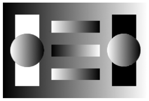
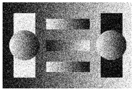
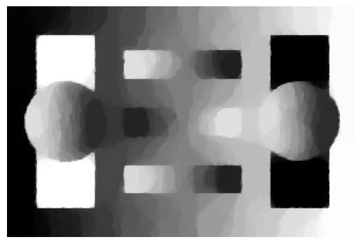
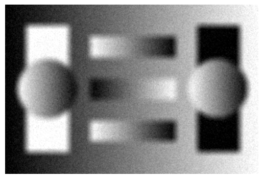
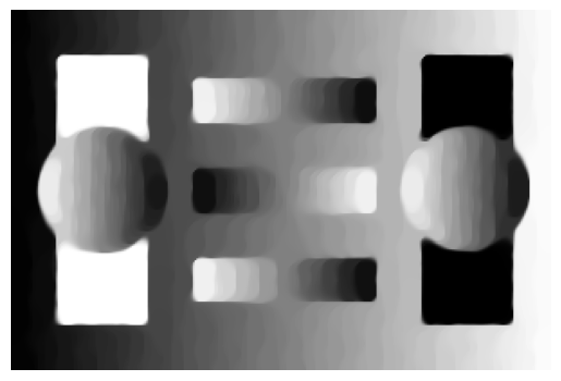
To ensure that any biases from algorithms under evaluation are avoided, the “exact” solution is calculated using an independent high-precision solver, in particular, the MOSEK solver from the CVXpy library [12, 13], see Figure 1.
Both the ProjGD and ProxSkip algorithms use the stepsize , where is the Lipschitz constant of . For every iteration, we monitor the error between the iterate and estimated exact solution . We use and 50000 iterations as a stopping criterion.
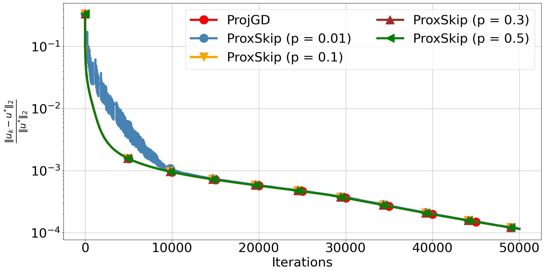
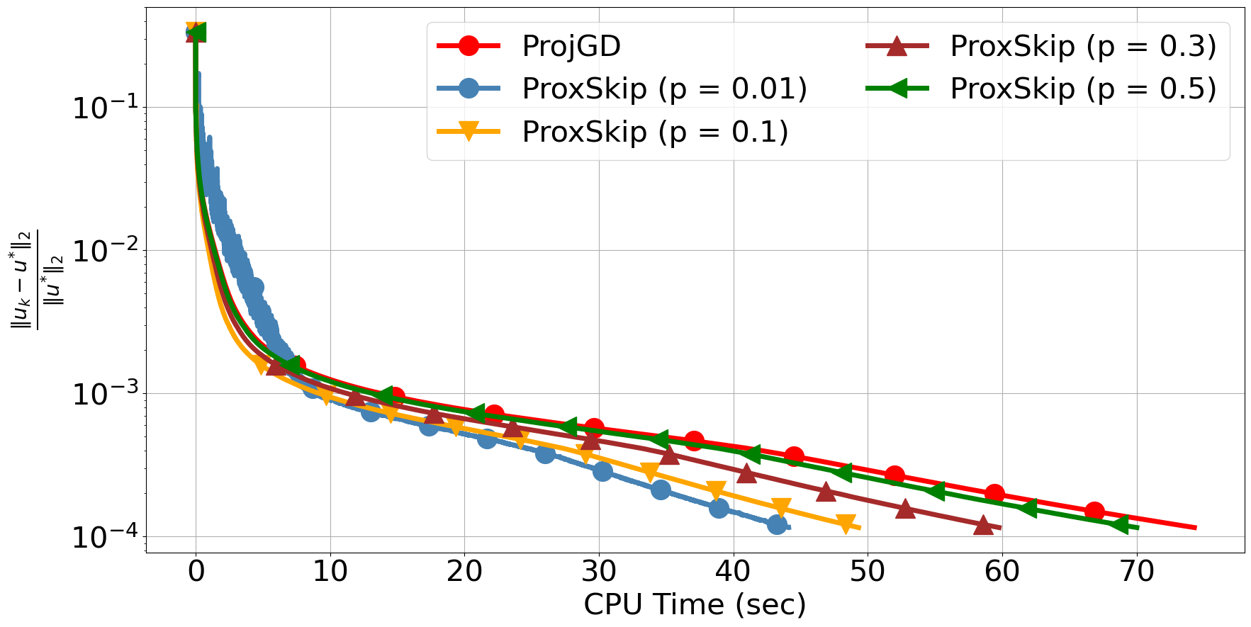
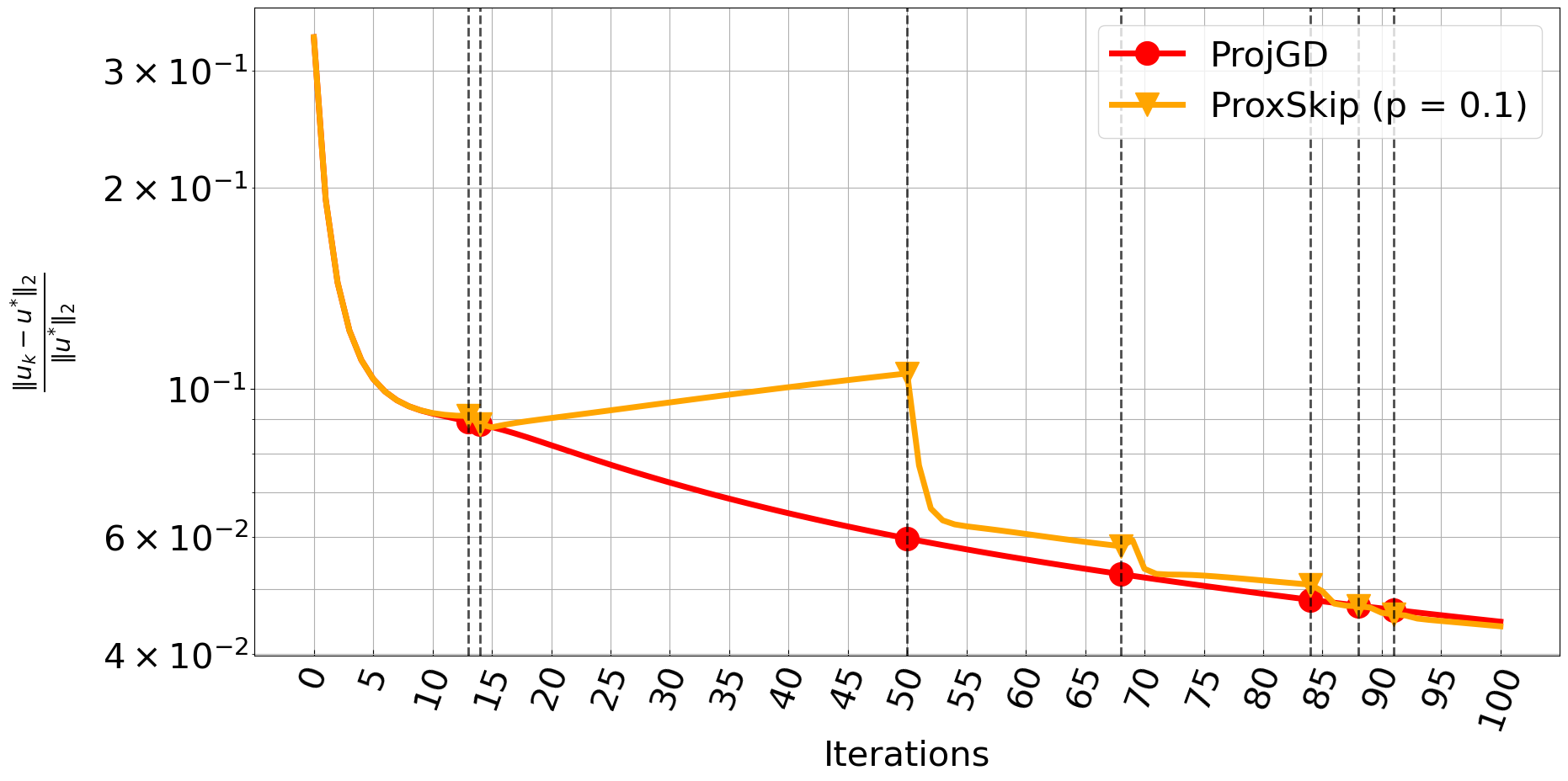
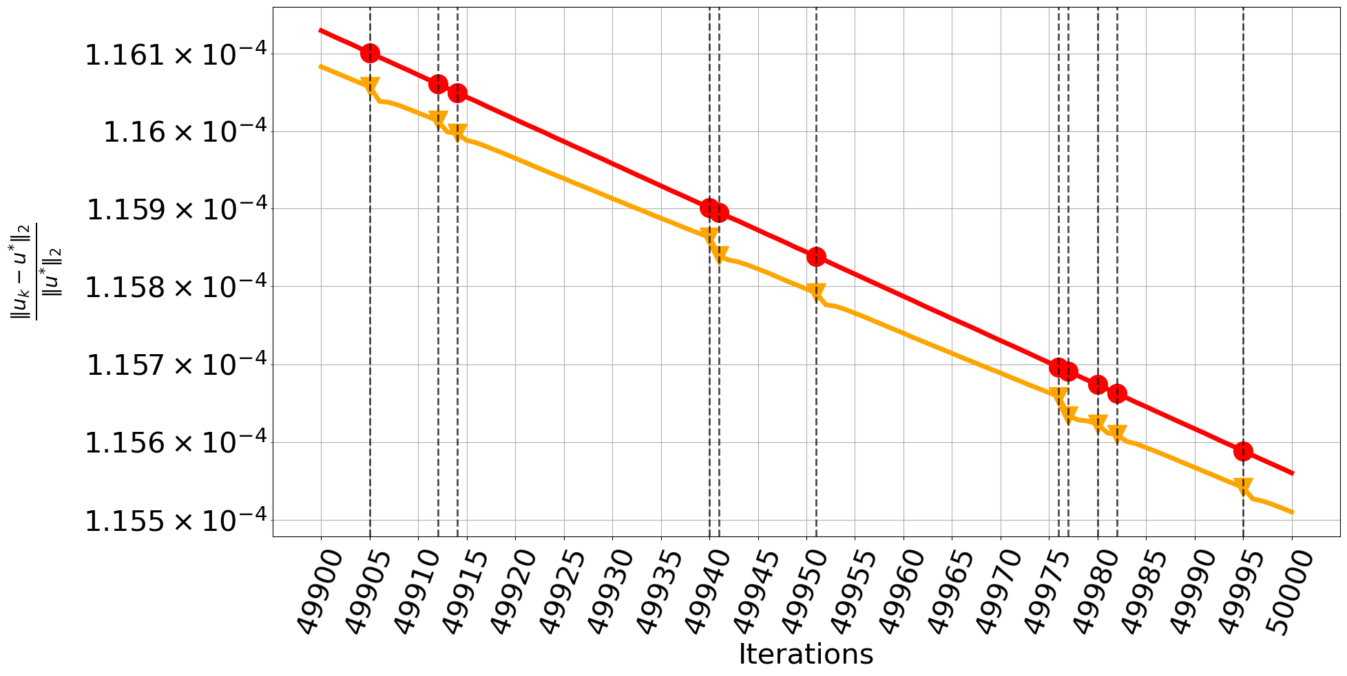
In Figure 2 (top-right), it can be observed that these two algorithms are almost identical in terms of the error. Note that ProxSkip and ProjGD coincide only when . Indeed, one can detect some discrepancies during first 100 iterations, which quickly dissipate with only a few applications of the projection , see bottom row of Figure 2. In Figure 2 (top-left), we plot the error with respect to CPU time. The shown CPU time is the average over 30 independent runs of each algorithm. We observe a clearly superior performance of ProxSkip, for all values of . This serves as a first demonstration of the advantage of ProxSkip in terms of computational time without affecting the quality of the image. In Section 3, we present a more emphatic computational impact using heavier proximal steps.
2.2 Dual TV denoising with strong convexity
In order to be consistent with the convergence theory of ProxSkip where strong convexity is a requirement, one can add a small quadratic term to the objective function. This is a commonly used in imaging applications and allows the use of accelerated versions of first-order methods. For the (6) problem this results in
| (8) |
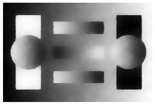
It is known that the corresponding primal problem of (8) is the standard Huber-TV denoising [7] which involves a quadratic smoothing of the -norm around an -neighbourhood of the origin. Among other effects, this reduces the staircasing artifacts of TV, see last image of Figure 1.
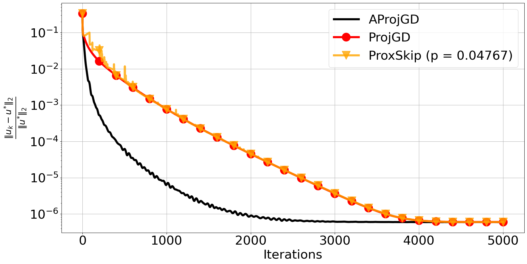
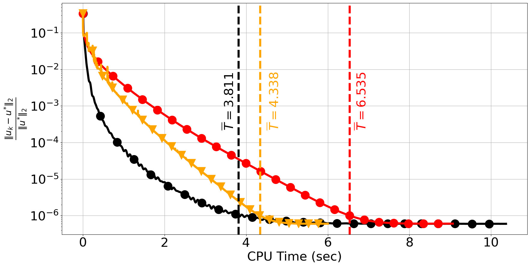
We repeat the same experiment as in the previous section for (8) with 5000 iterations and over 30 independent runs of the algorithm, using the probability , given by (4). This results in on average using only 215 projection steps during 5000 iterations. In addition to ProjGD, we also compare its accelerated version, denoted by AProjGD [14] which is essentially Algorithm 1 with the acceleration step of Algorithm 3. In Figure 3 (left), we observe that AProjGD performs better than both ProjGD and ProxSkip with respect to iteration number. While a similar behaviour is observed with respect to the CPU time, see Figure 3 (right), the average time for AProjGD and ProxSkip to reach a relative error less than is nearly identical. One would expect a similar speed-up when AProjGD is combined with skipping techniques but we leave this for future research.
3 ProxSkip in imaging problems with heavy proximals
3.1 TV deblurring
We now consider more challenging imaging tasks, involving proximal operators that do not admit closed form solutions, and which thus require computationally intensive iterative solvers.
We start with a deblurring problem in which is a convolution operator, see Figure 4.
We solve (5) and compare ISTA, FISTA and ProxSkip with different values of . Here the proximal operator corresponds to a TV denoiser for which we employ AProjGD with a fixed number of iterations as an inner iterative solver, see next section for other feasible options. In the framework of inexact regularisation another option is to terminate the inner solver based on some metric and predefined threshold [15]. As noted therein, the number of required inner iterations typically increases up to , as the outer algorithm progresses, leading to higher computational costs over time. To explore both the computationally easy and hard cases, we run the inner solver with 10 and 100 iterations, and use a warm-start strategy. Warm-start is a vital assumption for inexact regularisation as it avoids semi-convergence, where the error stagnates and fails to reach high precision solutions. To avoid biases towards proximal-gradient based solutions, the “exact” solution is computed using 200000 iterations of PDHG with diagonal preconditioning [16]. Outer algorithms are terminated if either 3000 iterations are reached or the relative distance error is less than . The reported CPU time is averaged over 10 runs.
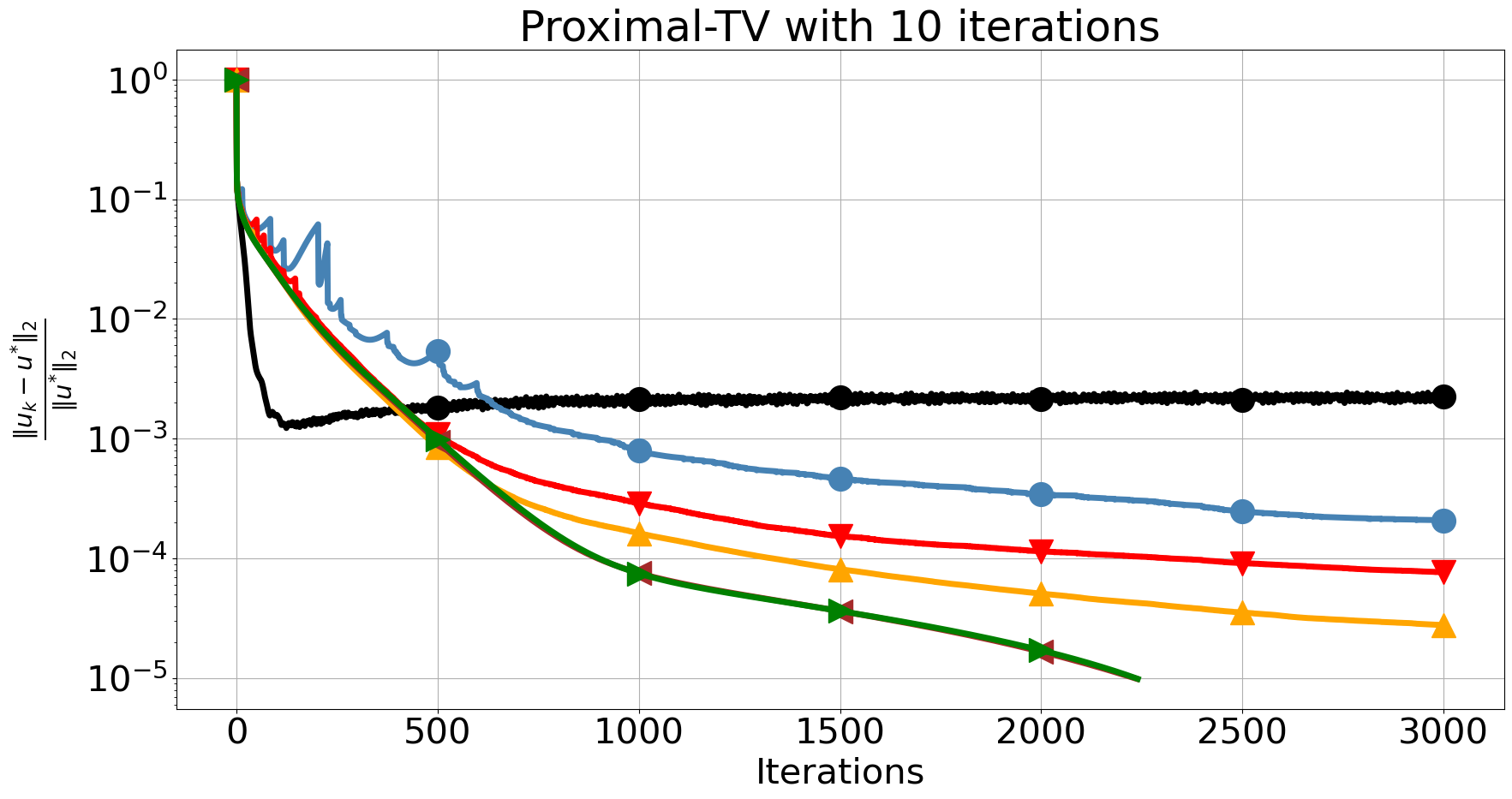
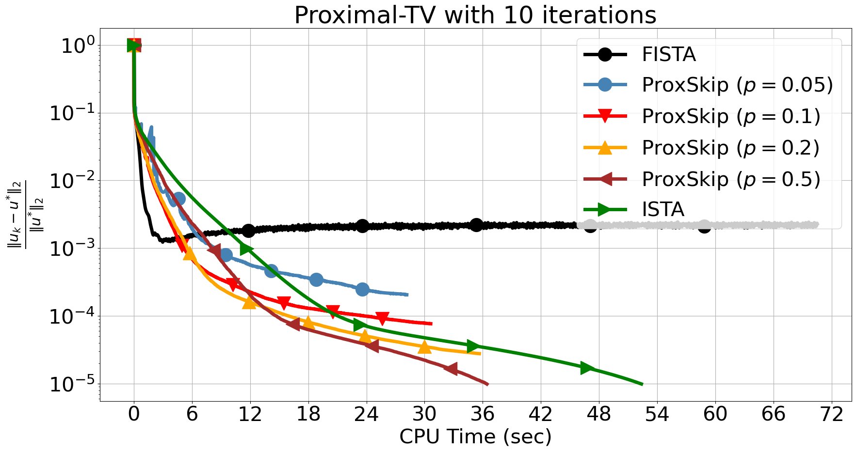
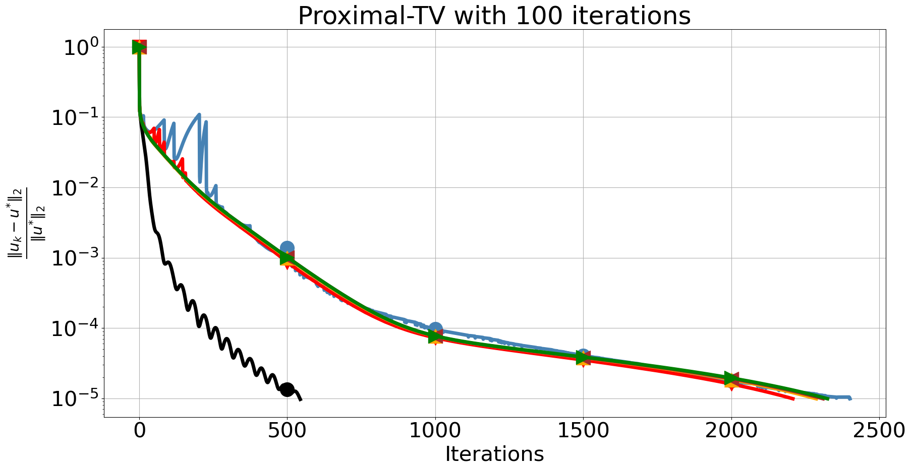
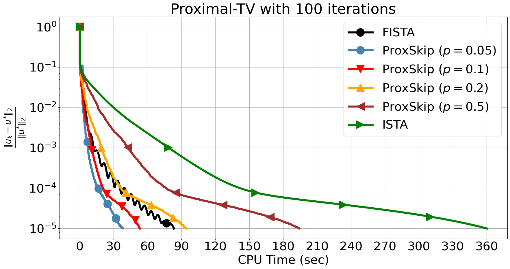
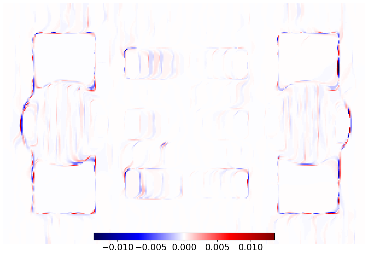
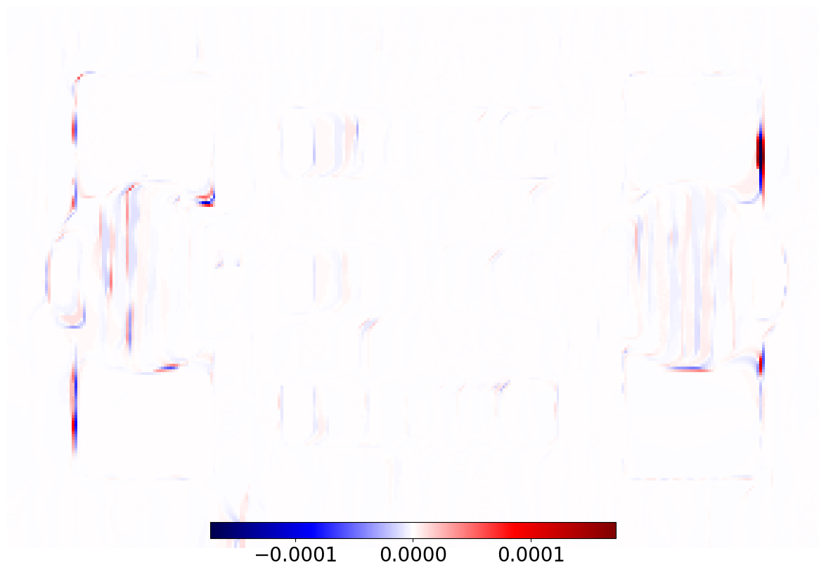
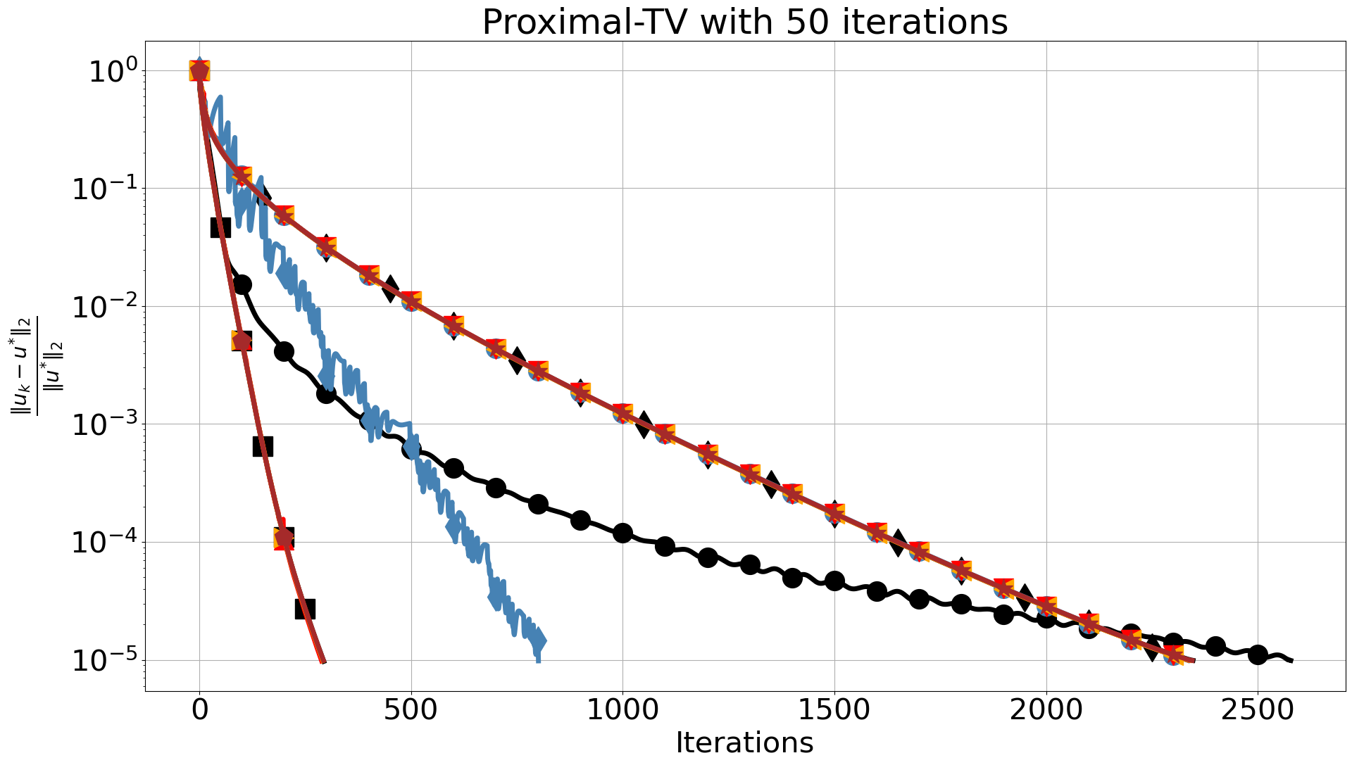
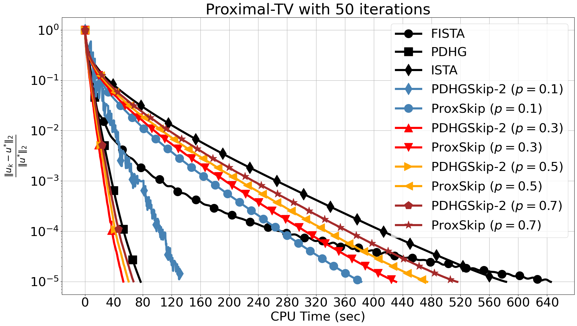
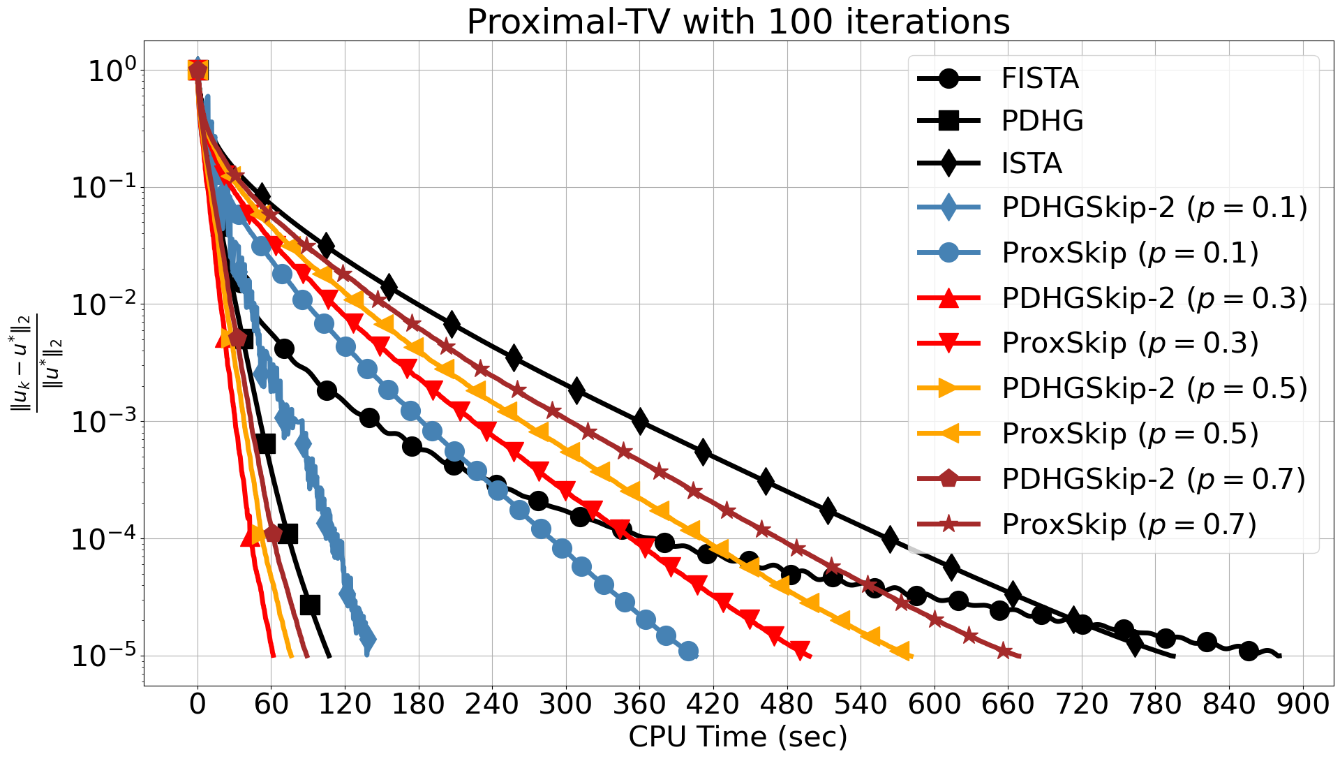
In Figure 5, we first observe that solving the inner TV problem with 10 iterations seriously affects the convergence of FISTA. Notably, ProxSkip versions are less affected even though besides the error introduced by the inexact solver, there is also an error from skipping the proximal. By raising the number of inner iterations to 100, and thus increasing the accuracy of the inner solver, we observe that FISTA exhibits an early decay albeit with some oscillations and it terminates after around 500 iterations, reaching an accuracy of , see Figure 5 (bottom-left). On the other hand, ISTA and the ProxSkip require many more iterations to reach the same level of accuracy. However, remarkably, in this regime ProxSkip is significantly faster, in terms of CPU time, than ISTA and even outperforms FISTA when and , see Figure 5 (bottom-right). In Table 1, we report all the information for the best three algorithms that outperformed FISTA with 100 inner iterations in terms of CPU time.
We note that there are versions of FISTA [17, 18, 19, 20] with improved performance, also avoiding oscillations. However, our purpose here is not an exhaustive comparison but to show that a simple version of ProxSkip outperforms the simplest version of FISTA. We anticipate the future development of more sophisticated skip-based algorithms including ones based on accelerated methods.
| Algorithm | Time Error (sec) | Iterations | # | Speed-up (%) |
|---|---|---|---|---|
| ProxSkip -10 () | 36.375 0.893 | 2233 | 1093 | 56.30 |
| ProxSkip -100 () | 39.43 0.664 | 2399 | 123 | 21.0 |
| ISTA -10 | 52.295 1.369 | 2237 | 2237 | 37.10 |
| FISTA - 100 | 83.205 4.933 | 543 | 543 | 0.0 |
3.2 PDHGSkip
Skipping the proximal can also be applied to primal-dual type algorithms. Here, for convex and a bounded linear operator , the optimisation framework is
| (9) |
In[21], a skip-version of PDHG [7] was proposed, which we denote here by PDHGSkip-1. It allows not only to skip one of the proximal steps but also the forward or backward operations of , depending on the order of the proximal steps, see Algorithm 5. In step 4, a Bernoulli operator is used, defined as with probability and otherwise. Again, strong convexity of both and is required for convergence. However, our imaging experiments – in the absence of strong convexity – revealed a relatively slow performance, even with optimised step sizes and according to [21, Theorem 7],
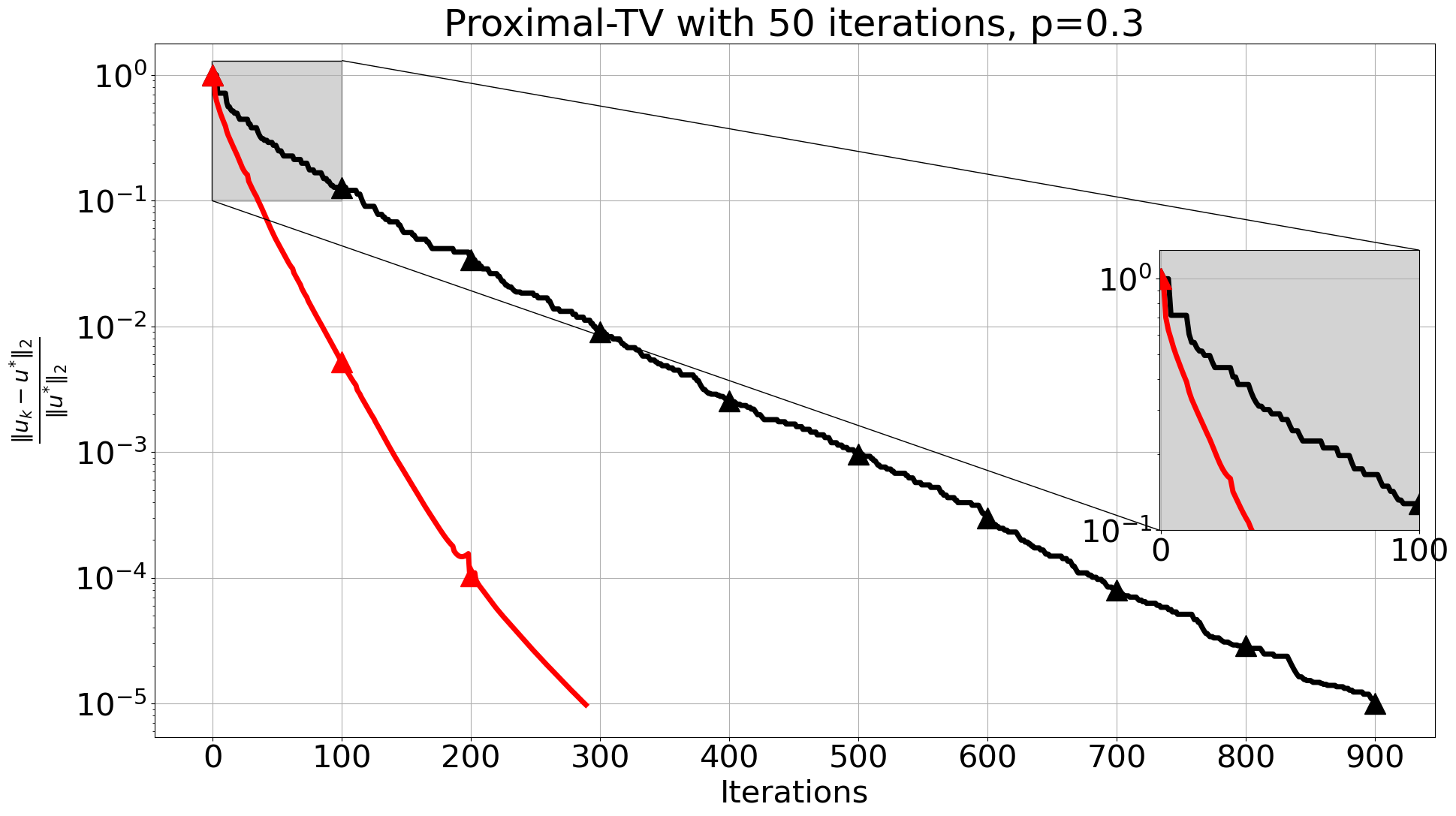
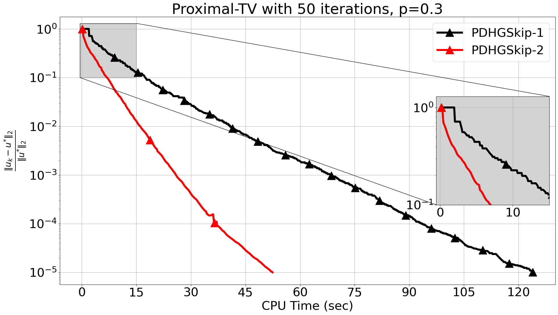
To address the slow convergence, we introduce a modification: PDHGSkip-2, see Algorithm 6. The difference to PDHGSkip-1 is that the adjoint and the proximal operator of are now separated, see steps 4-7. Note that in both versions, when the control variable vanishes and PDHG is recovered. To illustrate the difference of the two versions in practice, we show in Figure 6 a simple comparison on tomography, see next section for details. Apart from the clear acceleration of PDHGSkip-2 over PDHGSkip-1. We also observe a staircasing pattern for the relative error for PDGHSkip-1, see detailed zoom of the first iterations. This is expected since in most iterations, where the proximal step is skipped, one variable vanishes without contributing to the next iterate. Hence, the update remains unchanged.
In general, - problems can be solved using implicit or explicit formulations of PDHG. In the implicit case, is the term, and is the term. In the explicit case, is a separable sum of and composed with block operator and can be a zero function or a non-negativity constraint. Here, every proximal step (Steps 6, 9 in Algorithm 6) has an analytic solution. This significantly reduces the cost per-iteration, but also requires more iterations to reach a desired accuracy [22]. Inexact regularisation is usually preferred and typically reduces the number of iterations. Hence, the number of calls of the forward and backward operations of is reduced, which in certain applications gives a considerable speed-up.
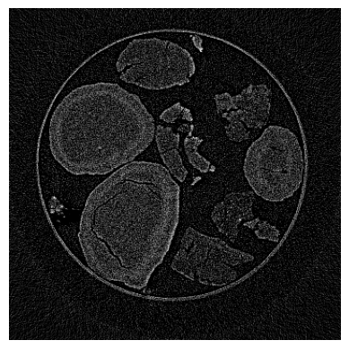
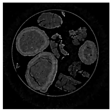
3.3 TV Tomography reconstruction with real-world data
For our final case study, we solve (5) under a non-negativity constraint for for a real-world tomographic reconstruction. Here is the discrete Radon transform and is a noisy sinogram of a real chemical imaging tomography dataset, representing post partial oxidation of methane reaction Ni-Pd/CeO2-ZrO2/Al2O3 catalyst [23, 24], see Figure 7. The initial dataset was acquired for 800 projection angles with 695695 detector size and 700 vertical slices. For demonstration purposes and to be able to perform multiple runs for computing more representative CPU times, we consider one vertical slice with half the projections and rebinned detector size. Same conditions for the inexact solver and stopping rules are used as in previous section. For these optimisation problems, one can use algorithms that fit both the general frameworks (2) and (9), see [25].
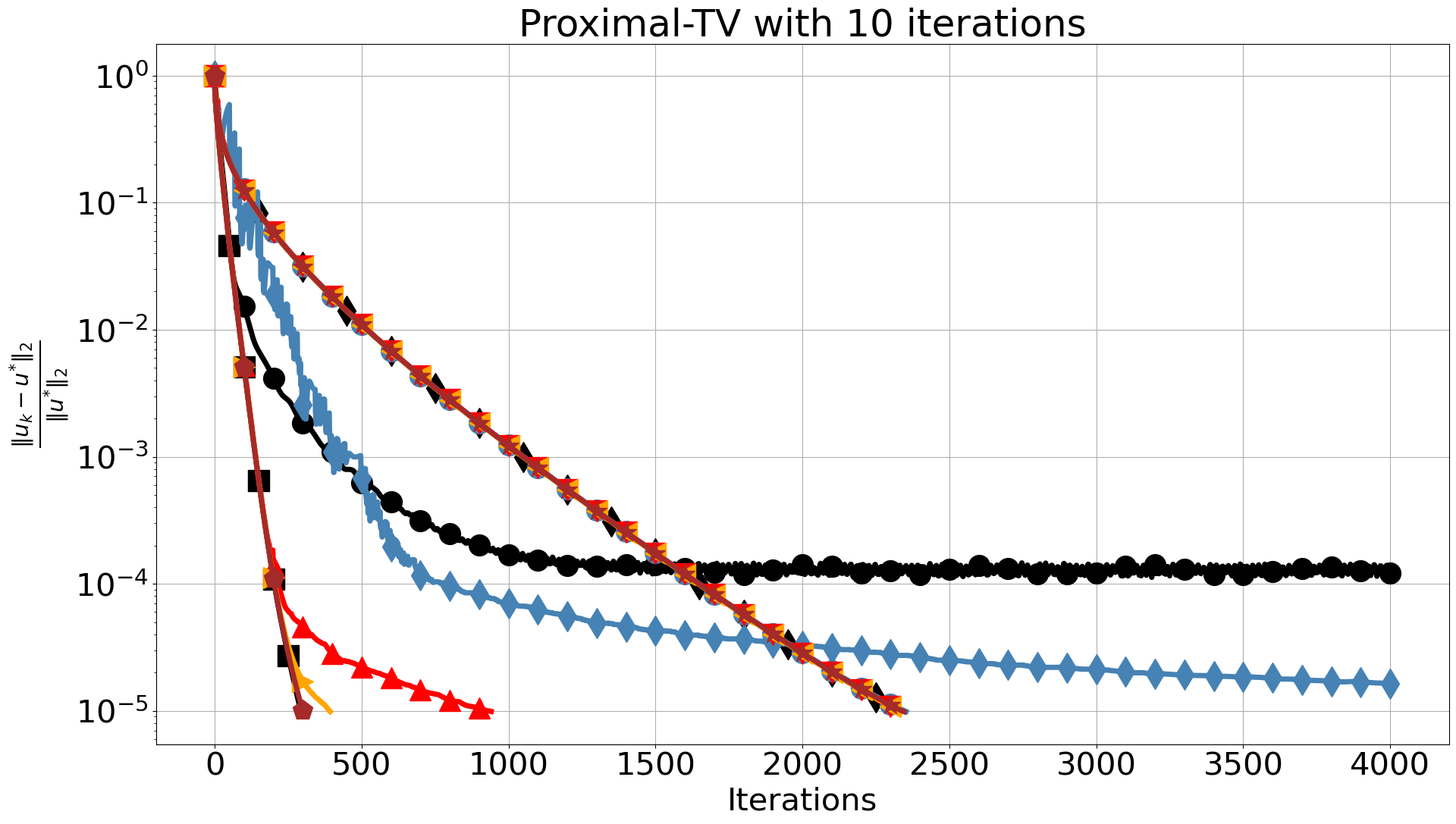
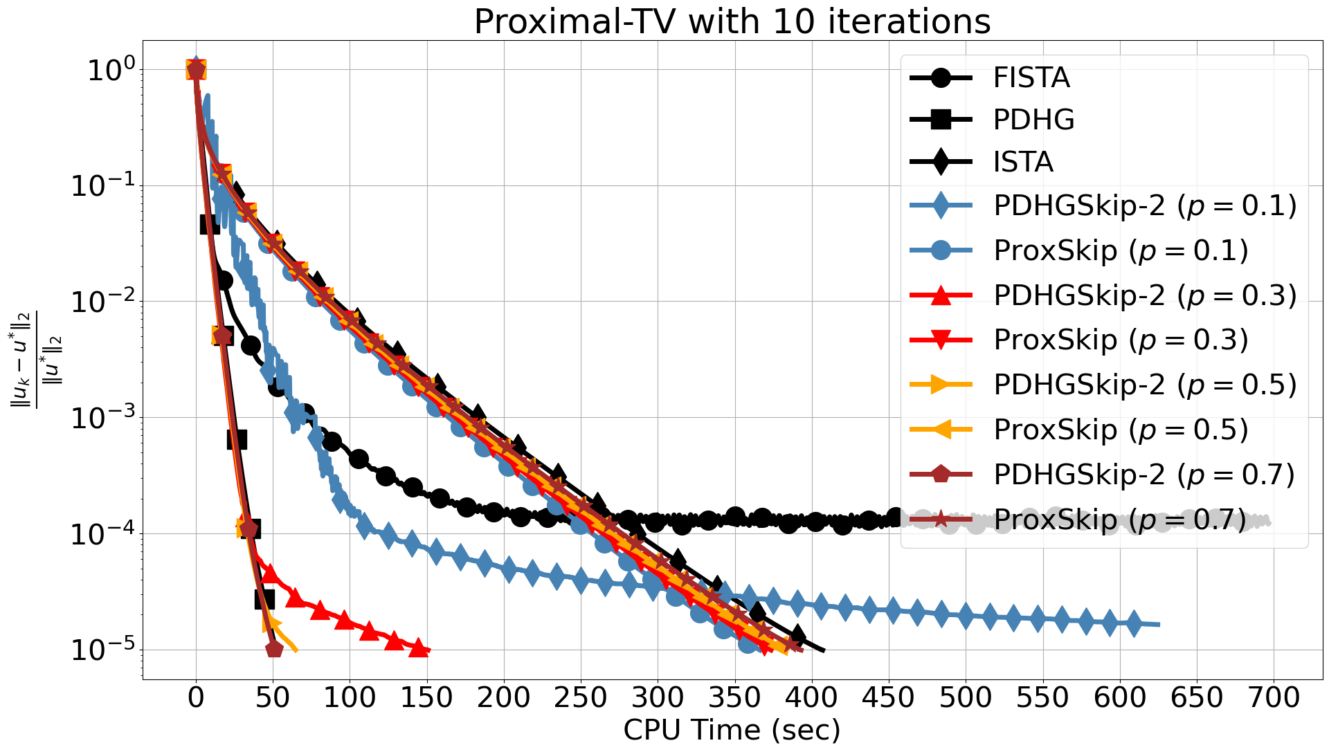
The two algorithms use the same values for step sizes and , satisfying . In the comparisons presented in Figure 8, we observe a similar trend for the proximal-gradient based algorithms as in Section 3.1. When we use 10 iterations for the inner solver, FISTA fails to reach the required accuracy and stagnates, which is not the case for the ProxSkip algorithms even for the smallest . This is accompanied by a significant CPU time speed-up, which further increases when more inner iterations are used. In fact, by increasing the number of inner iterations, the computational gain is evident with around 90% speed-up compared to FISTA.
The best overall performance with respect to CPU time is achieved by PDHGSkip-2. There, distance errors are identical to the case , in terms of iterations, except for the extreme case which oscillates in the early iterations. For 10 inner iterations and we observe a slight delay towards , due to error accumulation caused by skipping the proximal operator and limited accuracy of the inner solver. This is corrected when we increase the number of inner iterations. Moreover, we see no difference with respect to CPU time, for 10 inner iterations and . This is expected since the computational cost to run 10 iterations of AProjGD is relatively low. However, it demonstrates that we can have the same reconstruction using the proximal operator 70% of the time. Finally, the computational gain is more apparent when we increase the number of inner iterations hence the computational cost of the inner solver.
We note that such expensive inner steps are used by open source imaging libraries and are solved with different algorithms and stopping rules. In CIL [26, 27], the AProjGD is used to solve (6) with 100 iterations as default stopping criterion. In PyHST2 [28], AProjGD is used with 200 iterations and a duality gap is evaluated every 3 iterations. In TIGRE [29], the PDHG algorithm with adaptive step sizes is applied to (6), [30], with 50 iterations. In DeepInv 111https://github.com/deepinv/deepinv PDHG is applied to (5) (with ) with 1000 iterations and error distance between two consecutive iterates. Finally, in Tomopy[31], PDHG is applied to (5) (with ) and the number of iterations is specified by the user. All these default options are optimised and tested for particular real-world tomography applications like the ones encountered in synchroton facilities for instance. Alternatively, one can avoid inexact solvers for TV denoising [32]. There, the proximal is replaced by a combination of wavelet and scaling transforms and is computed using a componentwise shrinkage operator. Even in this case, we expect an improvement by skipping this operator. Overall, we anticipate a computational gain proportional to the cost savings achieved by omitting specific mathematical operations.

4 Code Reproducibility
The code and datasets need to reproduce the results will be made available upon acceptance of this paper. Also, we would like to highlight that all the experiments were tested in three different computing platforms under different operating systems. For this paper, we use an Apple M2 Pro, 16Gb without GPU use to avoid measuring data transferring time between the host and the device which can be misleading.
5 Discussion and Future work
In this paper, we explored the use of the ProxSkip algorithm for imaging inverse problems. This algorithm allows to skip costly proximal operators that are usually related to the regulariser without impacting the convergence and the final solution. In addition, we presented a new skipped version of PDHG, a more flexible algorithm, which can be useful when L-smoothness assumption is not satisfied, e.g., Kullback-Leibler divergence and its convergence is left for future work. Although, we demonstrated that avoiding computing the proximal leads to better computational times, this speed-up can be further increased when dealing with larger datasets and more costly regularisers, e.g. TGV. Additionally to the skipping concept, one can combine stochastic optimisation methods and different variance reduced estimators that use only a subset of the data per iteration. For example, in tomography applications, where the cost per iteration is mostly dominated by the forward and backward operations, one can randomly select a smaller subset of projection angles in addition to a random evaluation of the proximal operator. In this scenario, the cost per iteration is significantly decreased and from ongoing experiments outperformed deterministic algorithms in terms of CPU time. Finally, we note that we could achieve a further computational gain if we use the skipping concept to the inner solver as well. Notice for example that Algorithm (6) is designed by default to skip the proximal operator of . For the TV denoising problem, the projection step is avoided if
the dual formulation (6) is used, as presented in Section 2.1. On the other hand, the proximal operator, related to the fidelity term is avoided if we use the primal formulation.
Overall, proximal based algorithms presented here and possible future extensions open the door to revisiting a range of optimisation solutions for a plethora of imaging modalities, that were developed over the last decades, with the potential to greatly reduce actual computation times.
Acknowledgements
E. P. acknowledges funding through the Innovate UK Analysis for Innovators (A4i) program: Denoising of chemical imaging and tomography data under which the experiments were initially conducted. E. P. acknowledges also CCPi (EPSRC grant EP/T026677/1). Ž. K. is supported by the UK EPSRC grant EP/X010740/1.
References
- [1] K. Bredies and M. Holler, “Higher-order total variation approaches and generalisations,” Inverse Probl., vol. 36, no. 12, p. 123001, 2020.
- [2] K. Bredies, K. Kunisch, and T. Pock, “Total generalized variation,” SIAM J. Imaging Sci., vol. 3, no. 3, pp. 492–526, 2010.
- [3] K. M. Holt, “Total nuclear variation and Jacobian extensions of total variation for vector fields,” IEEE Trans. Image Process., vol. 23, no. 9, pp. 3975–3989, 2014.
- [4] S. Lefkimmiatis, A. Roussos, M. Unser, and P. Maragos, “Convex generalizations of total variation based on the structure tensor with applications to inverse problems,” in Scale Space and Variational Methods in Computer Vision, pp. 48–60, 2013.
- [5] P. L. Combettes and V. R. Wajs, “Signal recovery by proximal forward-backward splitting,” Multiscale Model. Sim., vol. 4, no. 4, pp. 1168–1200, 2005.
- [6] A. Beck and M. Teboulle, “A fast iterative shrinkage-thresholding algorithm for linear inverse problems,” SIAM J. Imaging Sci., vol. 2, no. 1, pp. 183–202, 2009.
- [7] A. Chambolle and T. Pock, “A first-order primal-dual algorithm for convex problems with applications to imaging,” J. Math. Imaging Vis., vol. 40, no. 1, pp. 120–145, 2011.
- [8] K. Mishchenko, G. Malinovsky, S. Stich, and P. Richtárik, “ProxSkip: Yes! Local gradient steps provably lead to communication acceleration! Finally!,” in PMLR 39, vol. 162, pp. 15750–15769, 2022.
- [9] A. Chambolle, “An algorithm for total variation minimization and applications,” J. Math. Imaging Vis., vol. 20, no. 1, pp. 89–97, 2004.
- [10] J.-F. Aujol, “Some first-order algorithms for total variation based image restoration,” J. Math. Imaging Vis., vol. 34, no. 3, pp. 307–327, 2009.
- [11] T. Pock, M. Unger, D. Cremers, and H. Bischof, “Fast and exact solution of total variation models on the GPU,” in IEEE Computer Society Conference on CVPR Workshops, pp. 1–8, 2008.
- [12] The MOSEK optimization toolbox for MATLAB manual. Version 10.1., 2024.
- [13] S. Diamond and S. Boyd, “CVXPY: A Python-embedded modeling language for convex optimization,” J. Mach. Learn. Res., vol. 17, no. 83, pp. 1–5, 2016.
- [14] Y. Nesterov, Introductory Lectures on Convex Optimization. Springer US, 2004.
- [15] J. Rasch and A. Chambolle, “Inexact first-order primal-dual algorithms,” Comput. Optim. Appl., vol. 76, no. 2, pp. 381–430, 2020.
- [16] T. Pock and A. Chambolle, “Diagonal preconditioning for first order primal-dual algorithms in convex optimization,” in 2011 International Conference on Computer Vision, pp. 1762–1769, 2011.
- [17] B. O’Donoghue and E. Candès, “Adaptive restart for accelerated gradient schemes,” Found. Comput. Math., vol. 15, no. 3, pp. 715–732, 2013.
- [18] A. Chambolle and C. Dossal, “On the convergence of the iterates of the ”fast iterative shrinkage/thresholding algorithm”,” J. Optim. Theory Appl., vol. 166, no. 3, pp. 968–982, 2015.
- [19] J. Liang, T. Luo, and C.-B. Schönlieb, “Improving Fast Iterative Shrinkage-Thresholding Algorithm: Faster, smarter, and greedier,” SIAM J. Sci. Comput., vol. 44, no. 3, pp. A1069–A1091, 2022.
- [20] J.-F. Aujol, L. Calatroni, C. Dossal, H. Labarrière, and A. Rondepierre, “Parameter-free FISTA by adaptive restart and backtracking,” SIAM J. Optim., vol. 34, no. 4, pp. 3259–3285, 2024.
- [21] L. Condat and P. Richtárik, “Randprox: Primal-dual optimization algorithms with randomized proximal updates,” in 11th ICLR, 2023.
- [22] M. Burger, A. Sawatzky, and G. Steidl, First Order Algorithms in Variational Image Processing, pp. 345–407. Springer International Publishing, 2016.
- [23] D. Matras, A. Vamvakeros, S. D. M. Jacques, M. di Michiel, V. Middelkoop, I. Z. Ismagilov, E. V. Matus, V. V. Kuznetsov, R. J. Cernik, and A. M. Beale, “Multi-length scale 5D diffraction imaging of Ni-Pd/CeO2-ZrO2/Al2O3 catalyst during partial oxidation of methane,” J. Mater. Chem. A, vol. 9, no. 18, pp. 11331–11346, 2021.
- [24] A. Vamvakeros, S. D. M. Jacques, M. Di Michiel, D. Matras, V. Middelkoop, I. Z. Ismagilov, E. V. Matus, V. V. Kuznetsov, J. Drnec, P. Senecal, and A. M. Beale, “5D operando tomographic diffraction imaging of a catalyst bed,” Nat. Commun., vol. 9, no. 1, 2018.
- [25] S. Anthoine, J.-F. Aujol, Y. Boursier, and C. Melot, “Some proximal methods for Poisson intensity CBCT and PET,” Inverse Probl. Imaging, vol. 6, no. 4, pp. 565–598, 2012.
- [26] J. S. Jørgensen, E. Ametova, G. Burca, G. Fardell, E. Papoutsellis, E. Pasca, K. Thielemans, M. Turner, R. Warr, W. R. B. Lionheart, and P. J. Withers, “Core Imaging Library - part I: a versatile Python framework for tomographic imaging,” Philos. Trans. A Math. Phys. Eng. Sci., vol. 379, no. 2204, p. 20200192, 2021.
- [27] E. Papoutsellis, E. Ametova, C. Delplancke, G. Fardell, J. S. Jørgensen, E. Pasca, M. Turner, R. Warr, W. R. B. Lionheart, and P. J. Withers, “Core Imaging Library - part II: multichannel reconstruction for dynamic and spectral tomography,” Philos. Trans. A Math. Phys. Eng. Sci., vol. 379, no. 2204, p. 20200193, 2021.
- [28] A. Mirone, E. Brun, E. Gouillart, P. Tafforeau, and J. Kieffer, “The PyHST2 hybrid distributed code for high speed tomographic reconstruction with iterative reconstruction and a priori knowledge capabilities,” Nucl. Instrum. Methods Phys. Res. B, vol. 324, pp. 41–48, 2014.
- [29] A. Biguri, M. Dosanjh, S. Hancock, and M. Soleimani, “TIGRE: a MATLAB-GPU toolbox for CBCT image reconstruction,” Biomed. Phys. Eng. Express, vol. 2, no. 5, p. 055010, 2016.
- [30] M. Zhu and T. Chan, “An efficient primal-dual hybrid gradient algorithm for total variation image restoration,” CAM Reports 08-34, UCLA, Center for Applied Math., 2008., no. 2, 2008.
- [31] D. Gürsoy, F. De Carlo, X. Xiao, and C. Jacobsen, “TomoPy: a framework for the analysis of synchrotron tomographic data,” J. Synchrotron Radiat., vol. 21, no. 5, pp. 1188–1193, 2014.
- [32] U. S. Kamilov, “Minimizing isotropic total variation without subiterations,” Mitsubishi Electric Research Laboratories (MERL), no. 2, 2016.