Width scaling of an interface constrained by a membrane
Abstract
We investigate the shape of a growing interface in the presence of an impenetrable moving membrane. The two distinct geometrical arrangements of the interface and membrane, obtained by placing the membrane behind or ahead of the interface, are not symmetrically related. On the basis of numerical results and an exact calculation, we argue that these two arrangements represent two distinct universality classes for interfacial growth: whilst the well-established Kardar-Parisi-Zhang (KPZ) growth is obtained in the ‘ahead’ arrangement, we find an arrested KPZ growth with a smaller roughness exponent in the ‘behind’ arrangement. This suggests that the surface properties of growing cell membranes and expanding bacterial colonies, for example, are fundamentally distinct.
Introduction.—Models of growing interfaces have been pivotal in developing a theoretical understanding of nonequilibrium statistical physics HHZ ; Krug97 ; KK10 ; Takeuchi17 . In particular, they have revealed that concepts of scaling and universality can apply beyond equilibrium critical phenomena to systems driven out of equilibrium. An important, robust universality class of growing interfaces is described by the Kardar-Parisi-Zhang (KPZ) equation, which reads
| (1) |
where is the height of an interface above a substrate and is a Gaussian white noise KPZ . It is well established that the width, , of a growing interface exhibits a dynamical scaling form FV
| (2) |
where the roughness exponent and dynamical exponent are determined by the universality class of the interface ( and for the KPZ equation in one dimension KPZ ; HHZ ; Krug97 ). Furthermore, universality also applies to higher moments of the height distribution KMHH .
More recently, major progress has been made in showing that the long time distribution of the height follows that of the largest eigenvalue of a random matrix drawn from an ensemble that depends on the geometry of the interface Johansson ; PS ; SS . Remarkably, these different sub-universality classes have been observed experimentally TS ; TSSS . Very recently exact results for random initial conditions have been obtained CFS17 ; MS17 as well as large deviations for the tails of the height distribution MKV16 ; LDMRS16 .
In this work we consider how the shape of a growing interface is affected by an impenetrable flat membrane whose vertical position fluctuates (see Fig. 1). As we note below, different physical situations correspond to two distinct arrangements: one in which the membrane is ahead of the growing interface, and one in which it is behind. We refer to these as arrangements A and B respectively. Since the KPZ equation is not invariant under height-reversal (), the two arrangements need not belong to the same universality class. On the basis of numerical results, an exact solution along a special line and crossover scaling analyses, we argue that this system has a rich phase diagram comprising two distinct phases where the interface is rough and bound to the membrane (in addition to an unbound and a smooth, bound phase). Specifically, rough interfaces in arrangement A are described by the usual KPZ scaling exponents, while those in arrangement B have distinct exponents and . We further argue that the latter behavior arises from dynamical arrest of the growing interface and therewith a generic mechanism for non-KPZ scaling.
Such deviations from KPZ behavior are of interest because the KPZ universality class is highly robust, due to the nonlinearity being the only relevant contribution to the dynamics of growing interfaces with local interactions at large length- and timescales for BS ; LP . Known exceptions tend to occur in rather special cases KS88 ; MKHZ89 ; DLSSa ; DLSSb ; WT90 ; KM92 , for example, when parameters are tuned to generate a leading nonlinearity at higher-order or when the noise is colored.
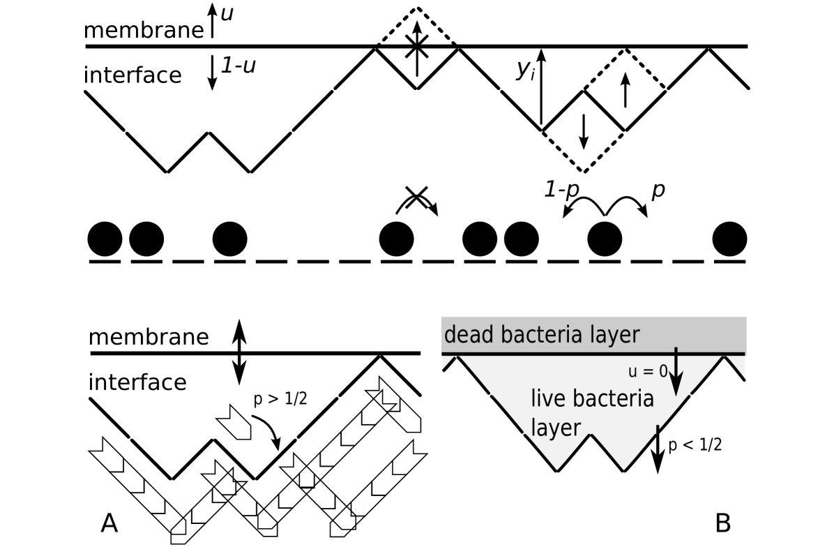
Model definition.—We now define the membrane-interface model that we study (see Fig. 1). The interface is of restricted solid-on-solid type MRSB86 ; KK89 and consists of upward or downward horizontal steps with periodic boundary conditions. We exploit a mapping to a system of particles with hard-core interactions where an occupied site, , represents a down-step of the interface (reading from left to right) and an empty site, , represents an up-step. On average once per unit time, each of the particles attempts to hop to a neighboring site (with the move rejected if the target site is occupied). Once a particle is chosen, it hops to the right with probability (which corresponds to a valley in the interface rising by two lattice sites) and to the left with probability . Free of a constraining membrane, the stationary state is one in which all particle configurations are equally likely LP ; MRSB86 : the interface then has the shape of a random walk, and its centre-of-mass moves upwards with velocity .
The dynamics of the free interface is modified by the presence of the membrane, a flat horizontal wall that is positioned above the interface (see Fig. 1). Once per unit time, the membrane attempts to move by one lattice site: upwards with probability , and downwards with probability . Thus in the absence of the interface, the membrane moves upwards with velocity . The interaction between the interface and membrane is modeled as follows: Any move, of either the interface or the membrane, that would cause them to overlap is forbidden. This occurs when there are points of contact between the membrane and interface. Note that the ‘ahead’ (A) and ‘behind’ (B) arrangements are both included in the model definition: (A) when , the interface’s growth is directed towards the membrane: i.e., any contacts with the membrane occur at interfacial peaks; (B) when the situation is reversed, and contacts lie at interfacial troughs. Since the height distribution functions of the free interface are asymmetric about the mean position Johansson ; PS ; SS , the effect of the membrane may be different in the two arrangements.
Arrangements A and B are also motivated by biophysical considerations. In cell growth, fluctuations of the cell membrane can allow a lamellipodium (a sheet of material packed with growing actin filaments) to expand into the space behind it Bray01 ; WBFEGM . At the same time, the membrane inhibits the lamellipodium, and the system can be modeled by arrangement A (see Fig. 1, lower-left panel). By contrast, some bacterial colonies advance through the division of living cells on the interface between the colony and its surroundings WSG17 . The consumption of nutrients by bacteria in the surface layer starve bacteria behind them: the boundary between the living and dead bacteria then forms a membrane behind the interface, as in arrangement B (Fig. 1, lower-right panel; BWpc ). More generally, the motion induced by growth behind a point-like fluctuating barrier has been modeled as a Brownian ratchet POO93 : the model we introduce here thus realizes a spatially-extended ratchet.
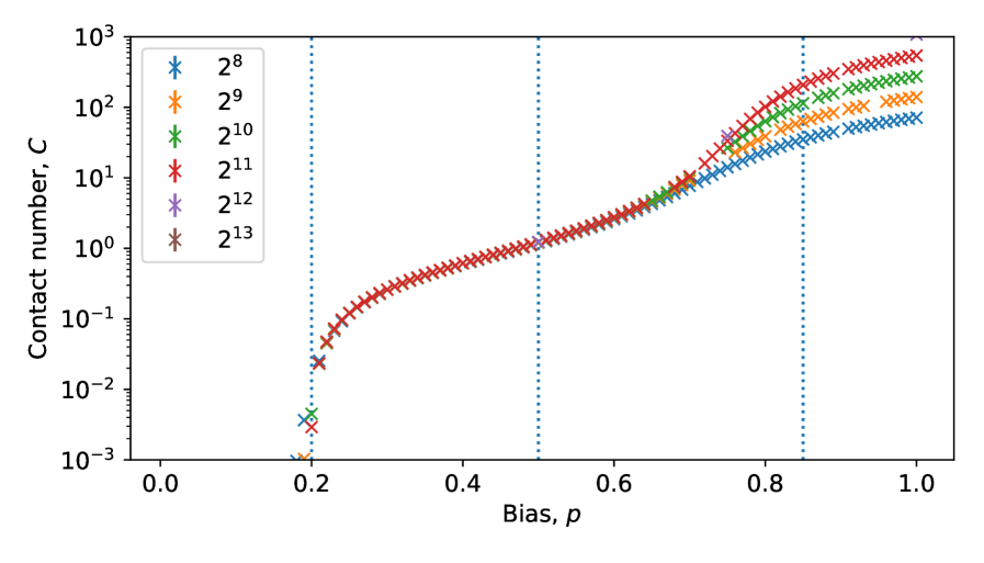
Phase diagram.— We establish the behavior for different values of and by direct Monte Carlo simulation. We define the separation as the distance between the interface and membrane at lattice point , and use an initial condition in which the interface lies flat against the membrane (i.e., is alternately and ). In characterizing the interfacial properties, it is important to distinguish between spatial averages, such as the centre-of-mass separation , and averages over the dynamical ensemble, which we denote with angle brackets. Then, is a random variable, and the width is defined by . We also consider the number of contacts between the membrane and interface, .
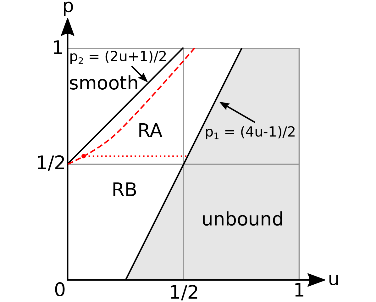
We summarize our findings from the simulations in the form of a phase diagram comprising four phases, Fig. 2. When , a free membrane and interface recede from each other. Thus for we expect an unbound phase where increases indefinitely, and the interface has KPZ scaling. Meanwhile, the membrane cannot move faster than , even when pushed by the interface. Therefore, if , we expect for a smooth phase where and . Simulation data (see Supplementary Figures) are consistent with these expectations and suggest that the boundary between the rough and smooth phase lies slightly below , as indicated in Fig. 2.
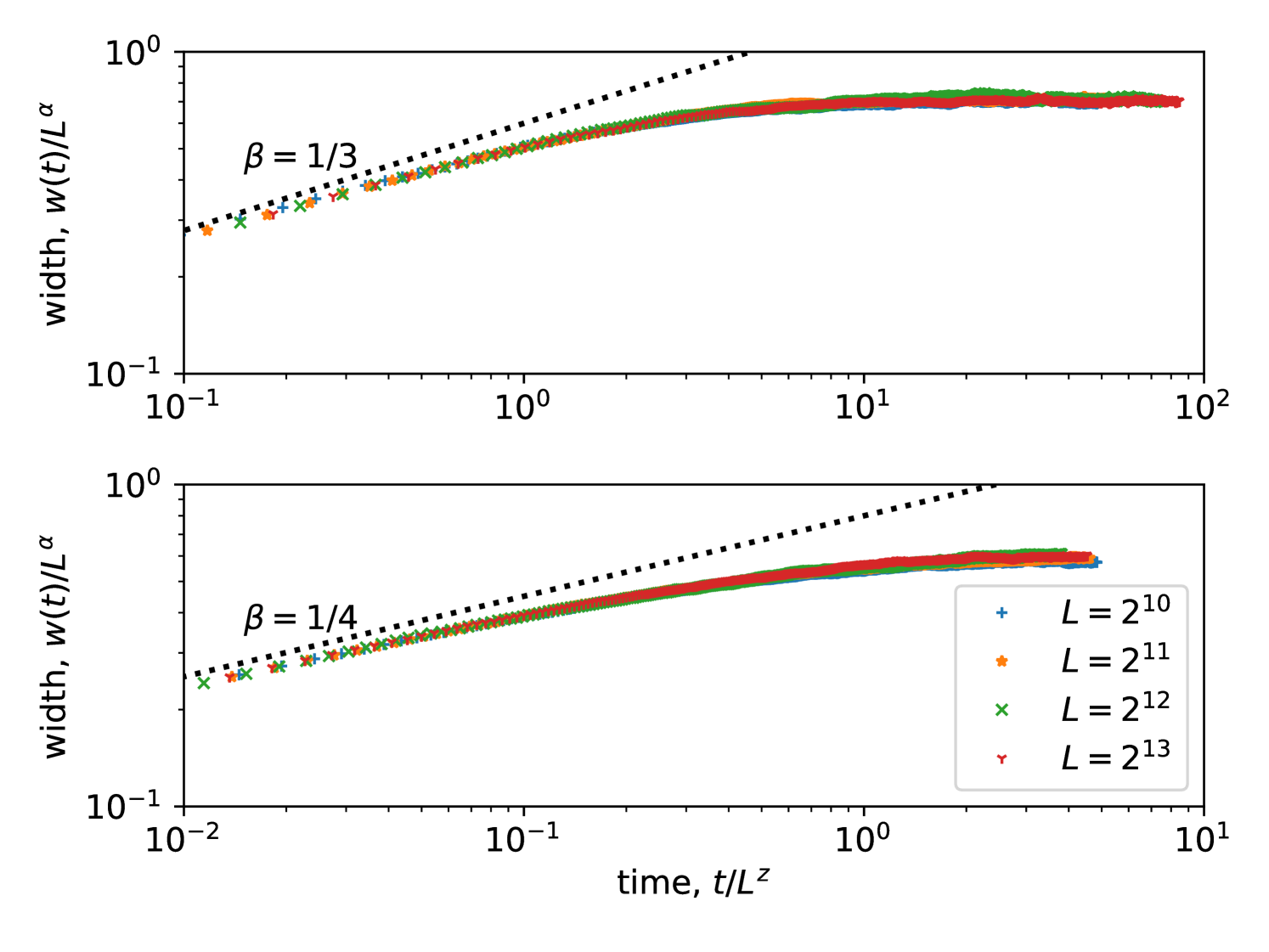
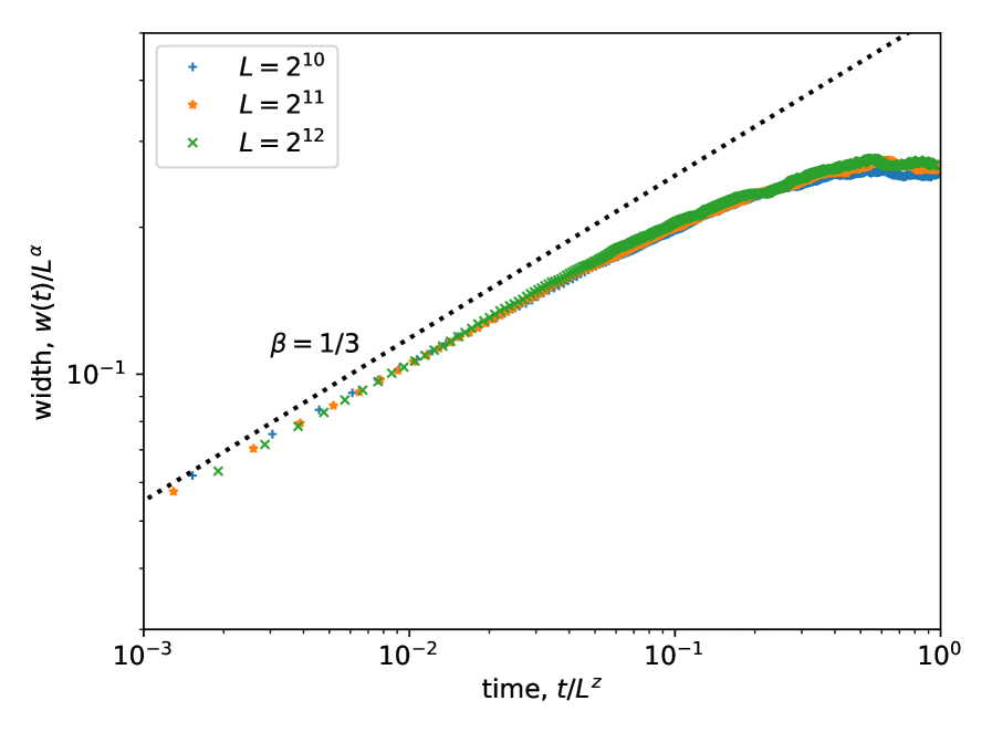
Of greatest interest are the two rough phases that lie between and , with a transition between them near . From the upper panel in Fig. 3 we find that for (arrangement B), the interface width scales as with an exponent , smaller than the usual KPZ exponent of . By contrast, for (arrangement A), is obtained (see Supplementary Figures). In both rough phases the contact count is i.e. the interface touches the membrane only a few times, with long excursions in between. In the following, we exclude the possibility that the non-KPZ exponent is a finite-size effect (as is sometimes the case BE2001 ) on the basis that an exact calculation, a crossover scaling analysis and a dynamical scaling collapse, all consistently point to . These analyses also suggest that in the limit the transition between the two rough phases occurs exactly at , where the switch between arrangements A and B takes place. We thus designate these phases as RA and RB, respectively.
Exact solution in the weakly-asymmetric limit.— We now show that the stationary state of the model is exactly solvable along the line
| (3) |
where particle hopping is weakly asymmetric ( as ) and is chosen so that detailed balance is satisfied. We first make a simple ansatz for the stationary distribution, , where is to be determined. For detailed balance to hold for membrane movement, we require which yields . Likewise, for the interface move we require yielding . Combining the two conditions gives
| (4) |
In the limit this corresponds to and . Thus as the exactly solvable line approaches from above for all . This suggests that the dotted line between RA and RB in Fig. 2 is a finite-size effect.
To determine the stationary height distribution , we introduce basis vectors that span the space of heights, and transfer matrix defined by and for . The expression
| (5) |
builds in the constraint that the height changes by exactly one unit along each bond on the lattice. Here we have used the fact that, for large , if is the largest eigenvalue of and and are the corresponding right and left eigenvectors.
The eigenvalue equation reads
| (6) |
We now make a continuum approximation , put where , and expand to leading non-trivial order for the case . We find
| (7) |
which, under a change of variable and transforms to Airy’s equation
| (8) |
The physical solution, which vanishes as , is . The appearance of the combination is almost sufficient to establish that characteristic lengthscale of the interface scales as , but to confirm this requires knowledge of how the eigenvalue behaves as . This we deduce from the boundary case in Eq. (6), which becomes
| (9) |
or equivalently where . This equation is satisfied by where is the largest real root of the Airy function. Substituting the resulting expression for back into the boundary condition reveals that . Putting this together we find
| (10) |
and a similar expression for the left eigenvector . Then, from (5) we finally obtain
| (11) |
which readily implies that , as . In particular, the width , confirming the roughness exponent in the vicinity of the line . In addition, which is consistent with a mean number of contacts that is independent of : .
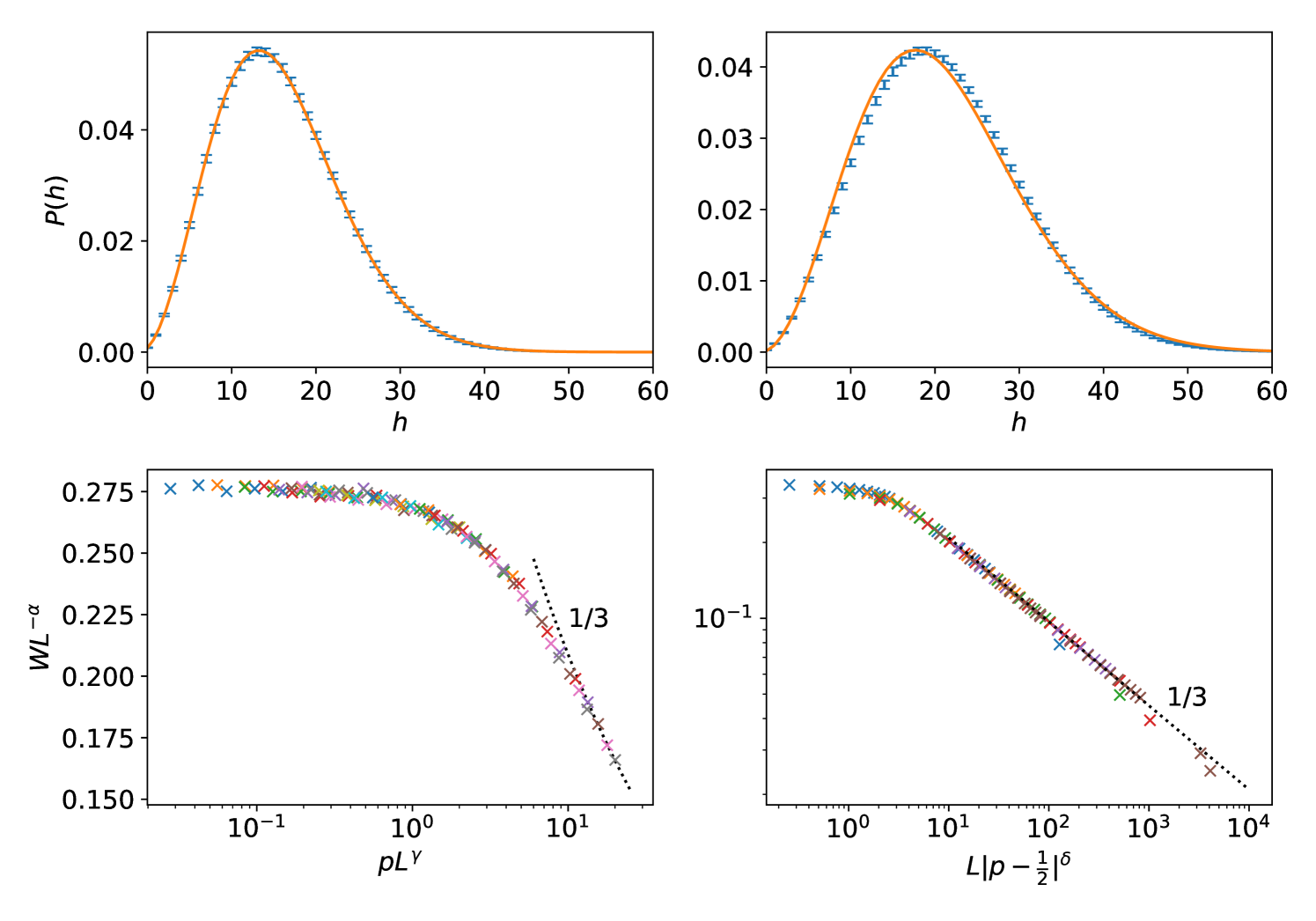
Roughness exponent in the RB phase.—We now present our main numerical evidence that the roughness exponent throughout the RB phase. First, we find that the Airy function height distribution (11), with and free parameters, fits the numerically-determined distribution both near the exactly-solvable line and deep in the RB phase (see upper panels of Fig. 4).
Second, crossovers to known behavior are also consistent with . At , the interface only grows downwards and cannot be affected by the membrane above it. Thus at the interface will exhibit the usual KPZ scaling with a roughness exponent . However, for in the RB phase, we expect and at finite there must be a crossover
| (12) |
where is a crossover exponent and is a scaling function which tends to a constant for small and has asymptotic behaviour for . For to go from along to within the RB phase we require . The data collapse in Figure 4 supports the scaling (12) and is consistent with and .
The system should also cross over to smooth phase behaviour for at . To study this we introduce a second crossover scaling function
| (13) |
and find that for there is a scaling collapse with . If the RB roughness exponent is , as claimed, we expect in this regime, which is confirmed by Fig. 4. The scaling form (13) further implies a divergence of the width in the smooth phase as , similar to a nonequilibrium wetting transition Hinrichsen1997 ; Hinrichsen2003 ; Barato2010 .
Dynamical arrest.— Finally, we return to the time dependence of the interfacial width, shown in Fig. 3, which provides a physical picture of the origin of the roughness exponent . Taking the scaling form (2), we can attempt to collapse for different by choosing different combinations of and . The best collapse is obtained when we assume that the early time growth, is unaffected by the membrane, and that the width saturates as with . In the RB phase, the initial growth should be in the KPZ class , which implies . On the transition line , the nonlinearity in (1) is absent, and an Edwards-Wilkinson (EW) early-time growth is expected, implying . The scaling collapse (Fig. 3) is consistent with both expectations and suggests that the effect of the membrane is to prematurely arrest the growth of the interface. The fact that different exponents are obtained for lends further credence to this being the true transition line.
Conclusion.— In this paper we have introduced a simple model of an interface interacting with a membrane: the presence of the membrane obstructs the growth of the interface when they are in contact. We have a determined a phase diagram that contains an unexpected phase RB in which the membrane is weakly bound to the interface but the roughness exponent of the interface is rather than the usual (for both KPZ and EW interfaces) value of . Evidence that this is the true asymptotic is provided by an exact solution along a special line (3), where detailed balance holds, and various scaling analyses.
It would be of great interest to observe the dynamical arrest experimentally, for example, in the context of growing bacterial colonies that motivated arrangement B. Such experimentally-relevant interfaces would usually be two-dimensional (2D), however we expect similar phenomena to occur in 2D as for the one-dimensional case: preliminary simulations Francesco in 2D for indicate a transition from a smooth to a rough phase RA with the same scaling (2) for the width but with exponent values corresponding to 2D KPZ , . Of further interest would be to investigate the 2D analogue of phase RB and associated exponents, however simulation times for the 2D single-step model with are known to become prohibitive KK89 .
Many other open questions remain. A more complete theory that explains why the dynamical arrest occurs only in arrangement B, where the membrane follows the interface from behind, is desirable. One possibility is that the asymmetric form of the universal height distribution of the growing KPZ interface Johansson ; PS ; SS implies that the interaction between interfacial peaks and troughs is fundamentally different. Finally, it should be noted that experimental interfaces such as those we invoke will naturally exhibit hydrodynamic couplings mediated by any fluid medium. Such couplings could generate effective long range interactions on the interface which, it is known, can change scaling properties BS .
Acknowledgements.
The authors thank Bartek Waclaw for interesting discussions on growing bacterial colonies and Davide Marenduzzo for interesting discussions on Brownian ratchets. J.W. acknowledges support from EPSRC under a studentship Grant No. EP/G03673X/1. J.W. and M.R.E. acknowledge the hospitality of the Weizmann Institute and M.R.E. acknowledges a Weston Visiting Professorship.References
- (1) Halpin-Healy T and Zhang Y-C Physics Reports 254, 215 (1995)
- (2) Krug J Advances in Physics 46, 139 (1997)
- (3) Kriecherbauer T, Krug J J. Phys. A: Math. Theor. 43 403001 (2010)
- (4) Takeuchi KA Physica A 504 77 (2018)
- (5) Kardar, M, Parisi, G, Zhang, Y-C Phys. Rev. Lett. 56 889 (1986)
- (6) Family F, Vicsek T J. Phys. A 18 L75 (1985)
- (7) Krug J, Meakin P, and Halpin-Healy T Phys. Rev. A 45 638 (1992)
- (8) Johansson K Commun. Math. Phys. 209 437 (2000)
- (9) Prähofer M, Spohn H Phys. Rev. Lett. 84 4882 (2000)
- (10) Sasamoto T, Spohn H Phys. Rev. Lett. 104 230602 (2010)
- (11) Takeuchi KA, Sano M Phys. Rev. Lett. 104 230601 (2010)
- (12) Takeuchi KA, Sano M, Sasamoto T, Spohn H Sci. Reports 1 34 (2011)
- (13) Chhita S, Ferrari P L, Spohn H Ann. Appl. Prob 28 1573 (2018)
- (14) Meerson B, Schmidt J J. Stat. Mech. 103207 (2017)
- (15) Meerson B, Katzav E, Vilenkin A Phys. Rev. Lett. 116 070601 (2016)
- (16) Le Doussal P, Majumdar S N, Rosso A, Schehr G Phys. Rev. Lett. 117 070403 (2016)
- (17) Barabasi A-L, Stanley H E Fractal Concepts in Surface Growth Cambridge University Press (1995)
- (18) Livi R and Politi P Nonequilibrium Statistical Physics Cambridge University Press (2017)
- (19) Krug J and Spohn H Phys. Rev. A 38 4271 (1988)
- (20) Medina E, Kardar M, Hwa T, Zhang, Y-C Phys. Rev. A 39 3053 (1989)
- (21) Derrida B, Lebowitz J, Speer ER, Spohn H Phys. Rev. Lett. 67 165 (1991)
- (22) Derrida B, Lebowitz J, Speer ER, Spohn H J. Phys. A: Math. Gen 24 4805 (1991)
- (23) Wolf DE, Tang L-H Phys. Rev. Lett. 65 1591 (1990)
- (24) Kandel D, Mukamel D EPL 20 325 (1992)
- (25) Meakin P, Ramanlal P, Sander LM, Ball RC Phys. Rev. A 34 5091 (1986)
- (26) Kim JM and Kosterlitz JM Phys. Rev. Lett. 62 2289 (1989)
- (27) Bray D 2001 Cell Movements: From Molecules to Motility 2nd edn (New York: Garland Publishing)
- (28) Wolff K, Barrett-Freeman C, Evans M R, Goryachev A B and Marenduzzo D Physical Biology, 11, 016005 (2014)
- (29) Wang X, Stone H. A., Golestanian R. New Journal of Physics, 19 125007 (2017)
- (30) Waclaw B, private communication.
- (31) Peskin C S, Odell G M, Oster G F, Biophysical Journal 65, 316 (1993)
- (32) Blythe RA, Evans MR Phys. Rev. E 64 051101 (2001)
- (33) Hinrichsen H, Livi R, Mukamel D, Politi A Phys. Rev. Lett. 79, 2710 (1997)
- (34) Hinrichsen H, Livi R, Mukamel D, Politi A Phys. Rev. E 68, 041606 (2003)
- (35) Barato A C J. Stat. Phys 138 728 (2010)
- (36) Cagnetta F private communication
Supplementary Figures