Wigner time delays and Goos-Hänchen shifts of 2D quantum vortices scattered by potential barriers
Abstract
We consider reflection and transmission of 2D quantum wavepackets with phase vortices (also known in optics as spatiotemporal vortex pulses) at potential step-like, delta-function, and rectangular barriers. The presence of a vortex significantly modifies the Wigner time delays and Goos-Hänchen shifts, previously studied for Gaussian-like wavepackets. In particular, the scattered wavepackets undergo non-zero time delays and lateral shifts even for purely real scattering coefficients, when the standard Wigner and Artmann formulae vanish. We derive analytical expressions for the vortex-induced times delays and spatial shifts of 2D vortices and verify these with numerical calculations of the Schrödinger equation. The time delays and shifts are resonantly enhanced in the vicinity of the critical-angle incidence for a step-like potential and near transmission resonances for a rectangular barrier.
the of and to
1 Introduction
Interference of waves in complex fields results in numerous nontrivial phenomena, such as phase singularities (vortices) and other topological wave structures [1, 2, 3], superoscillations and quantum weak values [4, 5, 6], time delays and superluminal propagation [7, 8, 9], beam shifts and Hall effects [10, 11, 12, 13, 14], etc. In some cases, these phenomena exhibit remarkable interplay with each other [15, 16, 17, 18]. Moreover, because of their universal wave nature, these effects appear equally in classical (e.g., optical or acoustic) and quantum (condensed-matter or free-particle) systems [19].
In this work, we examine a problem with remarkable interplay of the Wigner time delays [20], Goos-Hänchen (GH) shifts [21, 22], and phase vortices [1, 2] in a basic quantum system. Namely, we consider reflection and transmission of a 2D vortex wavepacket at various types of planar potential barriers within the Schrödinger equation.
Reflection and transmission of vortex beams, with the accompanying beam shifts, was thoroughly studied in optics [23, 24, 25, 26, 27, 28]. The presence of a vortex and the corresponding orbital angular momentum (OAM) dramatically modifies the beam shifts as compared to the case of Gaussian-like wavepackets. However, such problems were considered for the 3D setup where the vortex line and the corresponding OAM are aligned with the beam propagation direction (i.e., the beam carries a screw phase dislocation [1, 2]). Recently, there was considerable interest in spatiotemporal vortex pulses carrying the vortex line and OAM in the direction orthogonal to the propagation [29, 30, 31, 32, 33, 34, 35] (i.e., the pulse carries an edge phase dislocation [1, 2]). By examining reflection and refraction of such optical pulses at planar dielectric interfaces, we recently found that the spatiotemporal vortex and transverse OAM cause a novel effect of time delay (longitudinal pulse shift) and enables either subluminal or superluminal propagation of the reflected/transmitted pulses [36]. Remarkably, this vortex-induced time delay cannot be calculated from the standard Wigner formula [20, 7, 8, 9] which is valid only for Gaussian-like pulses without singularities and requires a temporal dispersion of the interface properties.
An important difference between the geometries of the longitudinal and transverse OAM/vortices is that the latter can naturally exist in planar 2D systems. In particular, 2D vortices carrying orthogonal OAM naturally appear in quantum condensed-matter systems, such as superfluids, BEC, quantum-Hall systems, 2D electron gas, and ferromagnets [37, 38, 39, 40, 41]. Furthermore, the Wigner time delays and superluminal tunneling were originally considered for quantum wavepackets [20, 7, 8, 9]. Therefore, the problem of vortex-induced time delays and shifts naturally arises for scattering (reflection or refraction) of a 2D quantum vortex at a potential barrier.
Here we examine this problem by considering the propagation and scattering of a 2D Laguerre-Gaussian-type vortex wavepacket within the Schrödinger equation with planar potential obstacles of different types: a step, a delta-function, and a rectangular barrier. We calculate the GH shifts and Wigner time delays of the reflected and transmitted wavepackets both in space-time (real or ‘linear’ shifts) and momentum-energy (imaginary or ‘angular’ shifts). We find novel vortex-induced contributions to the GH shifts and Wigner time delays of the scattered wavepackets. Most importantly, the vortex-induced time delays and lateral shifts appear even for purely real scattering coefficients where the standard Wigner time delay and GH effect vanish. These findings could be relevant to nontrivial transport properties of vortex states in 2D quantum systems.
2 Scattering of plane waves and Gaussian-like wavepackets
2.1 Schrödinger equation. Reflection and refraction of a plane wave
Throughout this work we deal with the 2D Schrödinger equation using the units :
| (1) |
where is the wavefunction, , , and is the potential. We consider three examples of potential barriers:
-
(A)
Step potential , where is the Heaviside step-function;
-
(B)
Delta-function barrier , where is the Dirac delta-function;
-
(C)
Rectangular barrier .
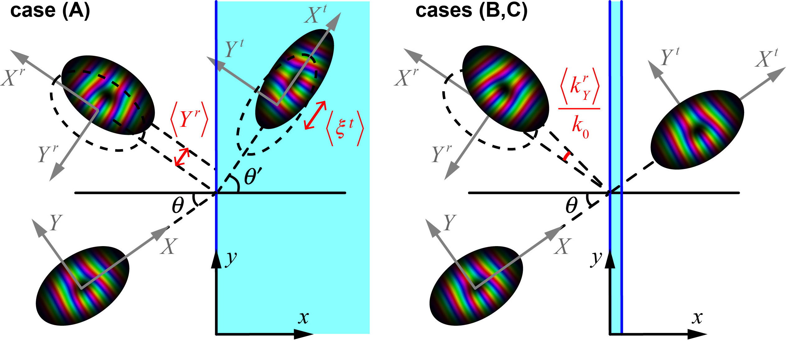
We will consider reflection and transmission of plane waves and wavepackets incident from the half-plane at the angle with respect to the -axis, see Fig. 1.
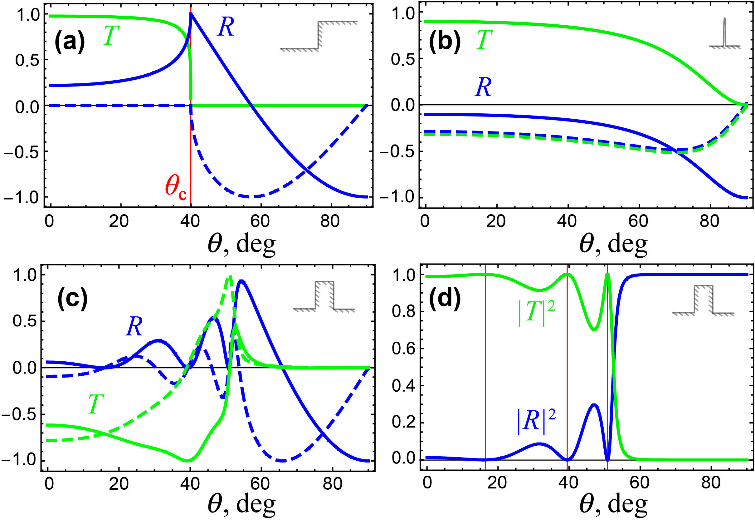
Consider first a single incident plane wave, , , with energy (frequency) , momentum (wave vector) , and dispersion following from Eq. (1). In the step-potential case (A), the reflected and transmitted waves, , , and , , have the same energies and wavevectors and , where and [19]. Applying the appropriate boundary conditions, i.e., the continuity of the total wavefunction and its normal derivative at , we obtain the scattering (reflection and transmission) amplitudes [see Fig. 2(a)]:
| (2) |
where . Note that the reflected and transmitted waves exist and acquire real amplitudes (2) in the regime of partial reflection/transmission, , while only the reflected propagating wave is generated in the regime of total reflection , where one should use , , and becomes complex.
In the delta-potential case (B), the incident wave is partially reflected/transmitted for all angles , whereas the transmitted wave has the same wavevector as the incident one, . The boundary conditions are: the continuity of the total wavefunction at and relation which follows from the integration of the Schrödinger equation (1) across the delta-barrier, . This results in the complex reflection and transmission amplitudes [see Fig. 2(b)]
| (3) |
Finally, in the case (C) of a finite rectangular barrier, consisting of two potential-step interfaces, the complex reflection and transmission amplitudes read [see Fig. 2(c)]
| (4) |
where is the normal wavevector component inside the barrier. Note that the scattering coefficients (2)–(4) satisfy the conservation law , and scattering by a rectangular barrier (C) exhibits resonances with total transmission , , Fig. 2(d).
2.2 Goos-Hänchen shifts and Wigner time delays for Gaussian-like wavepackets
We now consider reflection and transmission of a Gaussian wavepacket at the potential barriers of types (A)–(C). The incident wavepacket can be characterized by its Fourier spectrum (momentum representation)
| (5) |
Here and hereafter we use the coordinate frame with the -axis oriented along the propagation of the incident wavepacket, i.e., rotated by the angle with respect to the frame (see Fig. 1), is the central wavevector in the wavepacket, is the -width of the packet, whereas is its -length. We assume the wavepacket (5) to be paraxial and large as compared with the wavelength (i.e., semiclassical): . In the case (C) of a rectangular barrier we also assume that the wavepacket is much larger than the barrier width: ; this is to avoid numerous maxima in the reflected/transmitted signal due to the multiple reflections of a short pulse inside the barrier [9].
The real-space (coordinate) representation of the Gaussian wavepacket (5) is given by the Fourier integral
| (6) |
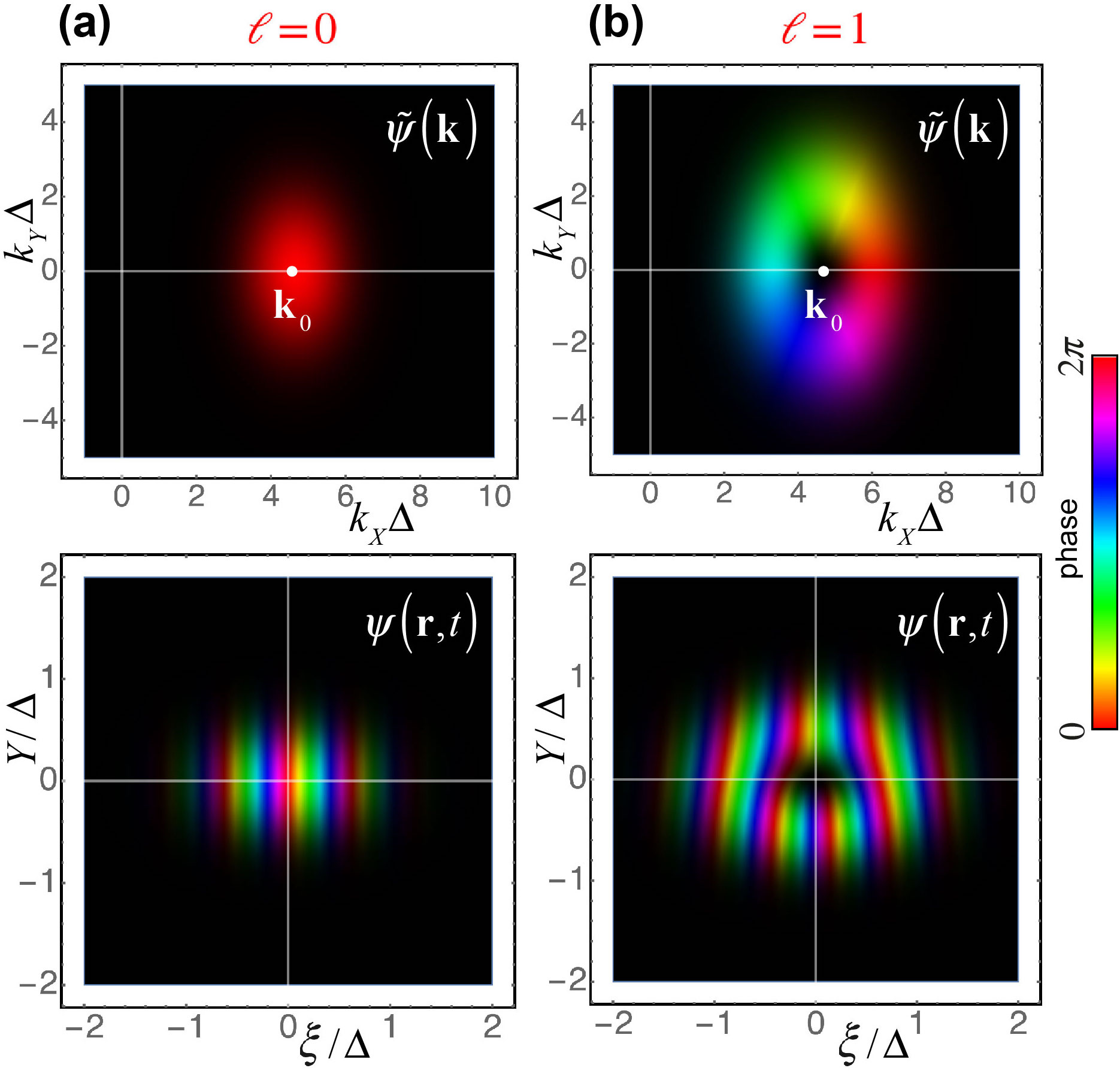
where , is the wavepacket-accompanying coordinate with the group velocity , and we neglected diffraction effects in the paraxial approximation. An example of the momentum-space and real-space wavefunctions (5) and (6) is shown in Fig. 3(a).
Spatial dispersion of the scattering coefficients (2)–(4), i.e., their dependence on the angle of incidence, , causes the GH shifts of the scattered wavepackets [21, 22, 10]. The linear (position) and angular (direction) GH shifts can be characterized by the mean transverse position and transverse momentum (with respect to the expected geometrical-optics or semiclassical trajectory) of the scattered wavepackets. The generalized Artmann formula [22, 10] yields
| (7) | |||
| (8) |
Here and hereafter the coordinates and wavevectors of the reflected and transmitted wavepackets are written in the coordinate frames accompanying the reflected and refracted wavepackets [10], the subscript “0” indicates that we deal with a Gaussian (no-vortex) wavepacket, in the case of step potential (A), and in the cases (B) and (C). The coordinate frames and schematics of some of the GH shifts are shown in Fig. 1. The linear shifts are non-diffractive effects appearing right after the scattering event, while the angular shifts accumulate additional spatial shifts proportional to the propagation distances [10, 43, 44, 45]. The GH shifts are well studied in optics and also in quantum systems [46, 47, 48, 49], although, to the best of our knowledge, the angular GH effect has never been discussed for quantum systems.
In analogy to the GH effect, the temporal dispersion of the scattering coefficients (2)–(4), i.e., their dependence on the energy of the incident wave, , results in the Wigner time delays of the scattered wavepackets [20, 7, 8, 9, 18].
| (9) | |||
| (10) |
Here denotes the time delay of the scattered wavepacket as compared to its expected arrival time, whereas is the shift of its mean energy/frequency with respect to the central energy of the incident wavepacket, . These are temporal counterparts of the linear and angular GH shifts, so that the energy shift accumulates an additional time delay proportional to the propagation time of the wavepacket. The Wigner time delays (9) and (10) can be equally regarded as spatial and angular shifts in the longitudinal wavepacket-accompanying coordinate and the corresponding wavevector component , where , , in the step-potential case (A) and in the other cases.
The coordinate/momentum GH shifts, Eqs. (7) and (8), and the Wigner time/frequency shifts, Eqs. (9) and (10), can be associated with the real/imaginary parts of complex values and . This duality and connections between the GH and Wigner effects were discussed in various contexts in Refs. [50, 51, 18] and is related to manifestations of complex quantum weak values [11, 12, 52, 18, 53, 6].
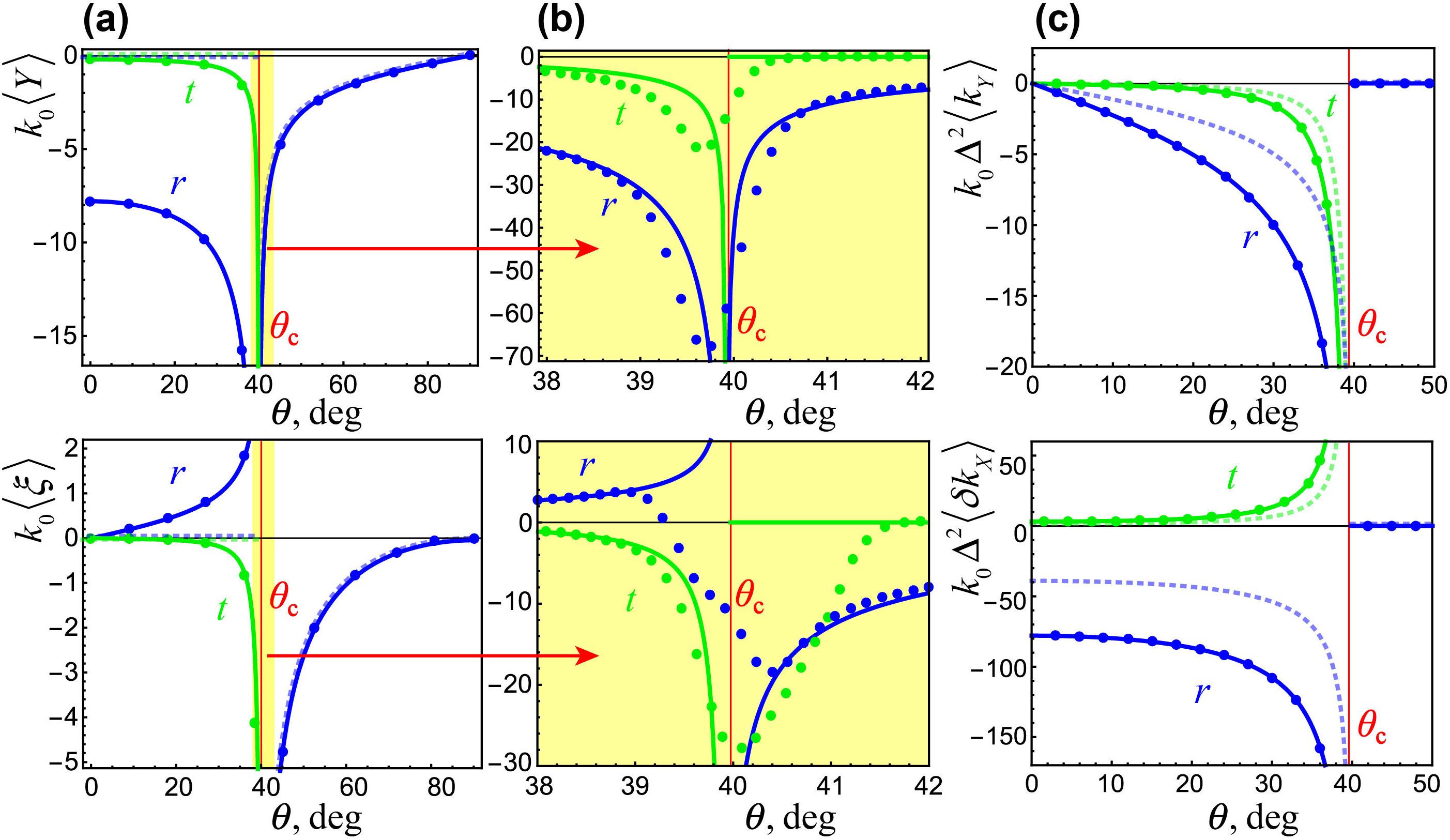
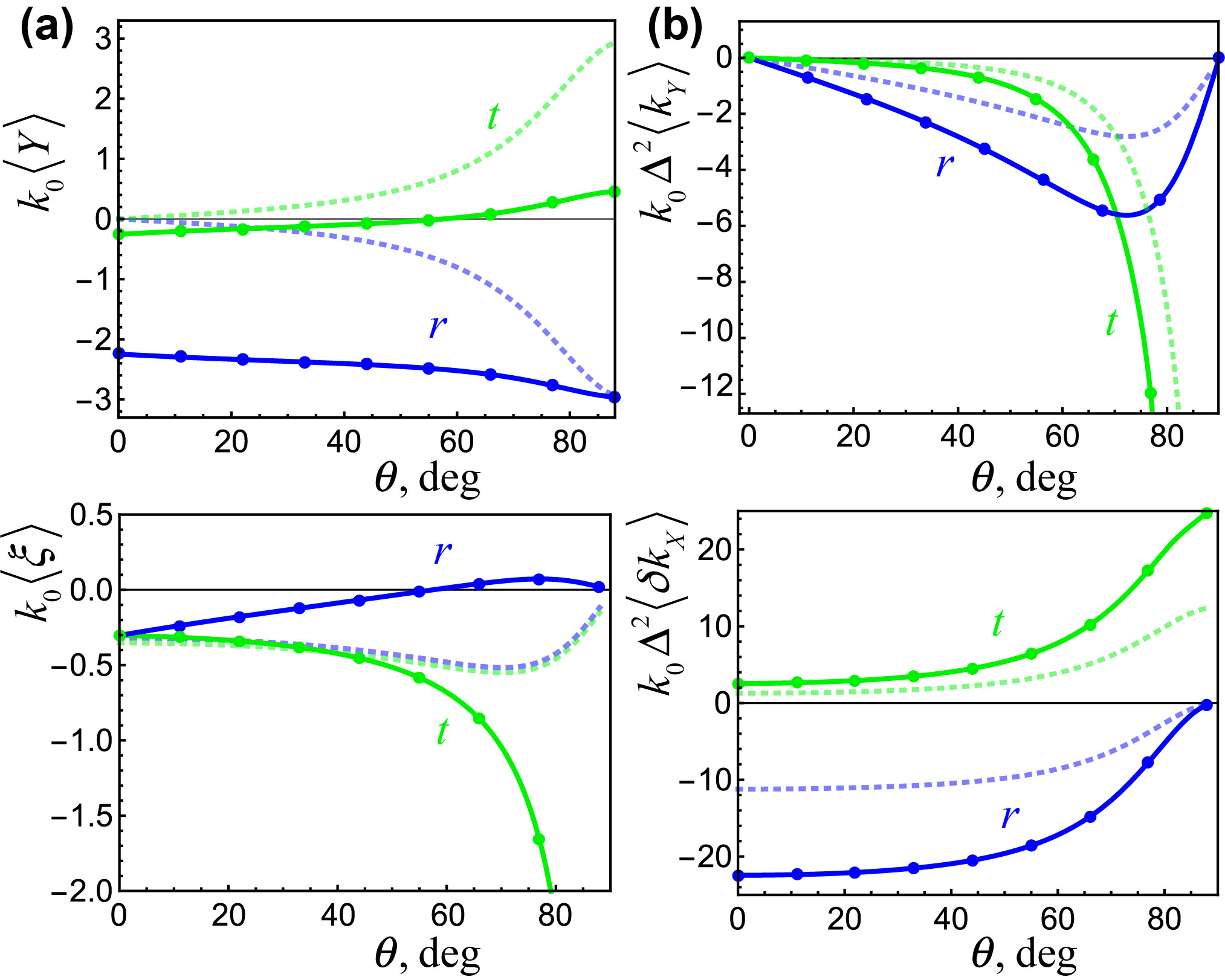
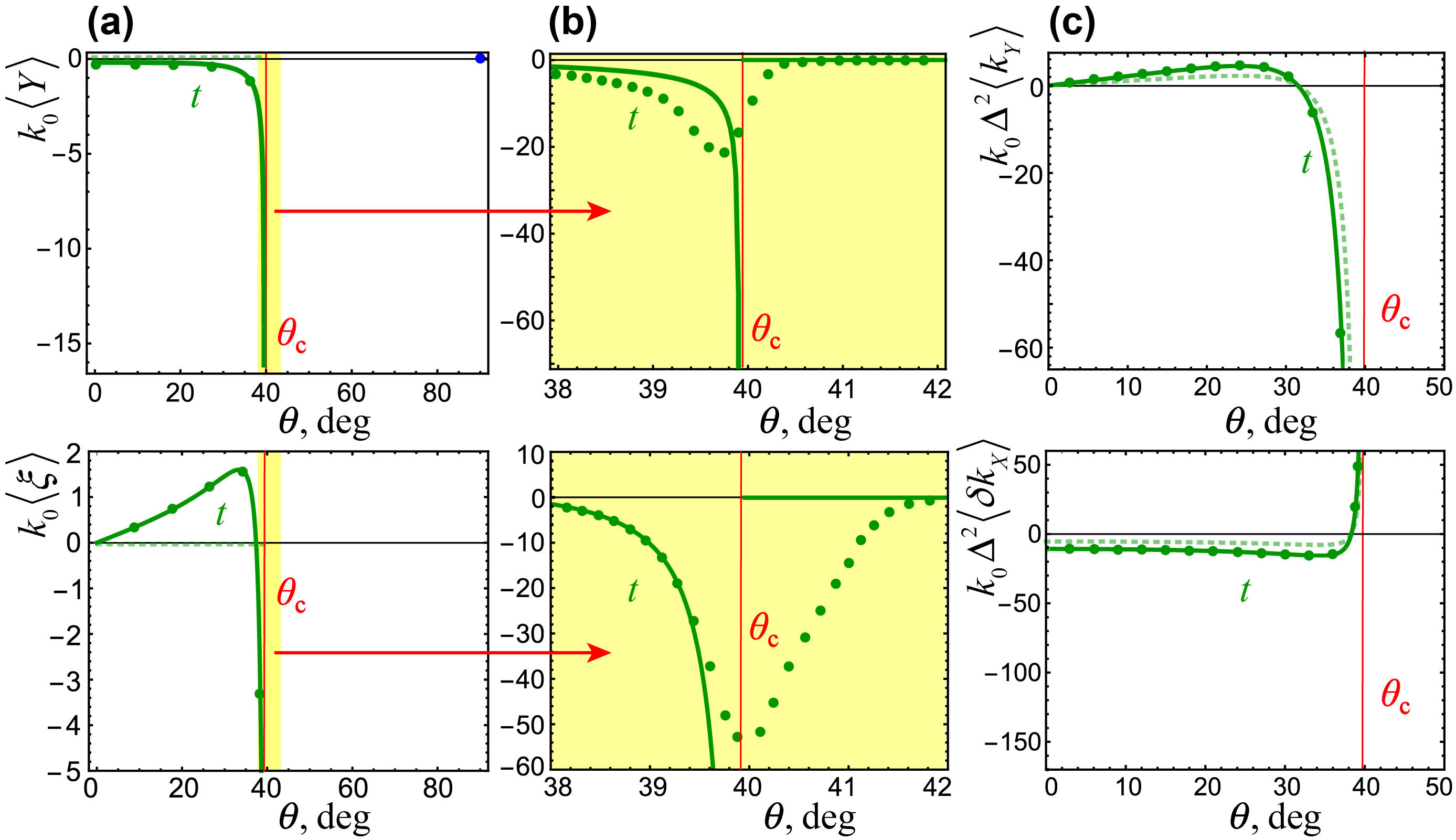
The GH shifts and Wigner time delays, Eqs. (7)–(10) versus the angle of incidence in specific cases of barriers (A)–(C) are shown in Figures 4–6 by dotted curves. Notice that the linear quantities and , Eqs. (7) and (9), vanish in the case of partial reflection and transmission at the step potential (A), , because the scattering coefficients (2) are purely real in this case. The angular quantities and , Eqs. (8) and (10), are generally nonzero in all cases (A)–(C). Importantly, the analytical expressions for the shifts and time delays can diverge at zeros of scattering coefficients: e.g., at the critical angle of incidence, , in the case (A) and near zeros of the reflection coefficient (transmission resonances) in the case (C). Approximate formulas (7)–(10) become inapplicable near such singularities, whereas the shifts/delays can exceed their typical values by several orders of magnitude [43, 24, 45, 54, 18, 55, 36]. This amplification of otherwise small effects is a manifestation of quantum weak measurements and superweak values [56, 18].
3 Scattering of 2D Laguerre-Gaussian-like vortices
We are now in the position to consider a 2D vortex wavepacket. We model it with the spatiotemporal Laguerre-Gaussian solution [36], which adds an edge phase singularity (vortex) of the integer order in the center of the Gaussian wavepacket (5) [see Fig. 3(b)]:
| (11) |
In the paraxial approximation, neglecting diffraction effects, the Fourier integral of Eq. (11) yields the real-space form of the propagating 2D vortex [29, 30, 31, 32, 33, 34, 35]:
| (12) |
For , the wavepacket (11) and (12) becomes the Gaussian wavepacket (5) and (6). For , the wavefunction (12) vanishes in the centre , has the probability density in the form of an elliptical ‘doughnut’ with the ratio of semiaxes , and a circulation of the probability current . The latter determines the normalized (per particle) OAM carried by the wavepacket and directed along the orthogonal -axis [29, 33, 36]:
| (13) |
An example of the vortex wavepacket (11) and (12) with is shown in Fig. 3(b).
When the vortex wavepacket (11) and (12) is scattered by a potential barrier, it experiences the GH shifts and Wigner time delays in the reflected and transmitted wavepackets. Here we examine how these effects are affected by the vortex in the incident packet. First, as was shown for optical vortex beams and spatiotemporal vortex pulses [26, 27, 36], the angular shifts are amplified with the factor of as compared to the shifts of Gaussian-type wavepackets, Eqs. (8) and (10), so that the additional vortex-induced wavevector and energy shifts are:
| (14) |
Second, the complex vortex structure in the wavepacket (12) produces a cross-coupling between the orthogonal Cartesian degrees of freedom. To describe it, we note that the reflected wavepacket will have a flipped vortex with the topological charge and vortex structure . Furthermore, in the potential-step case (A), the and dimensions of the transmitted wavepacket are modified by the factors and , respectively [10, 36]. This results in the transmitted vortex structure , where .
Next, we notice that the angular GH shifts , Eq. (8), can be regarded as imaginary shifts in real space [10, 26, 36, 44]: and . Substituting these imaginary shifts into the vortex forms of the corresponding scattered wavepackets, we find that they are equivalent to real -dependent shifts in the orthogonal -directions: and . In turn, these shifts are equivalent to the new vortex-induced time delays
| (15) |
In a similar manner, the angular Wigner shifts (10), , can be regarded as imaginary shifts in real space: and . Substituting these imaginary shifts into the vortex structures of the scattered wavepackets, we find that they are equivalent to real -dependent shifts in the orthogonal -directions:
| (16) |
These are novel vortex-induced GH shifts.
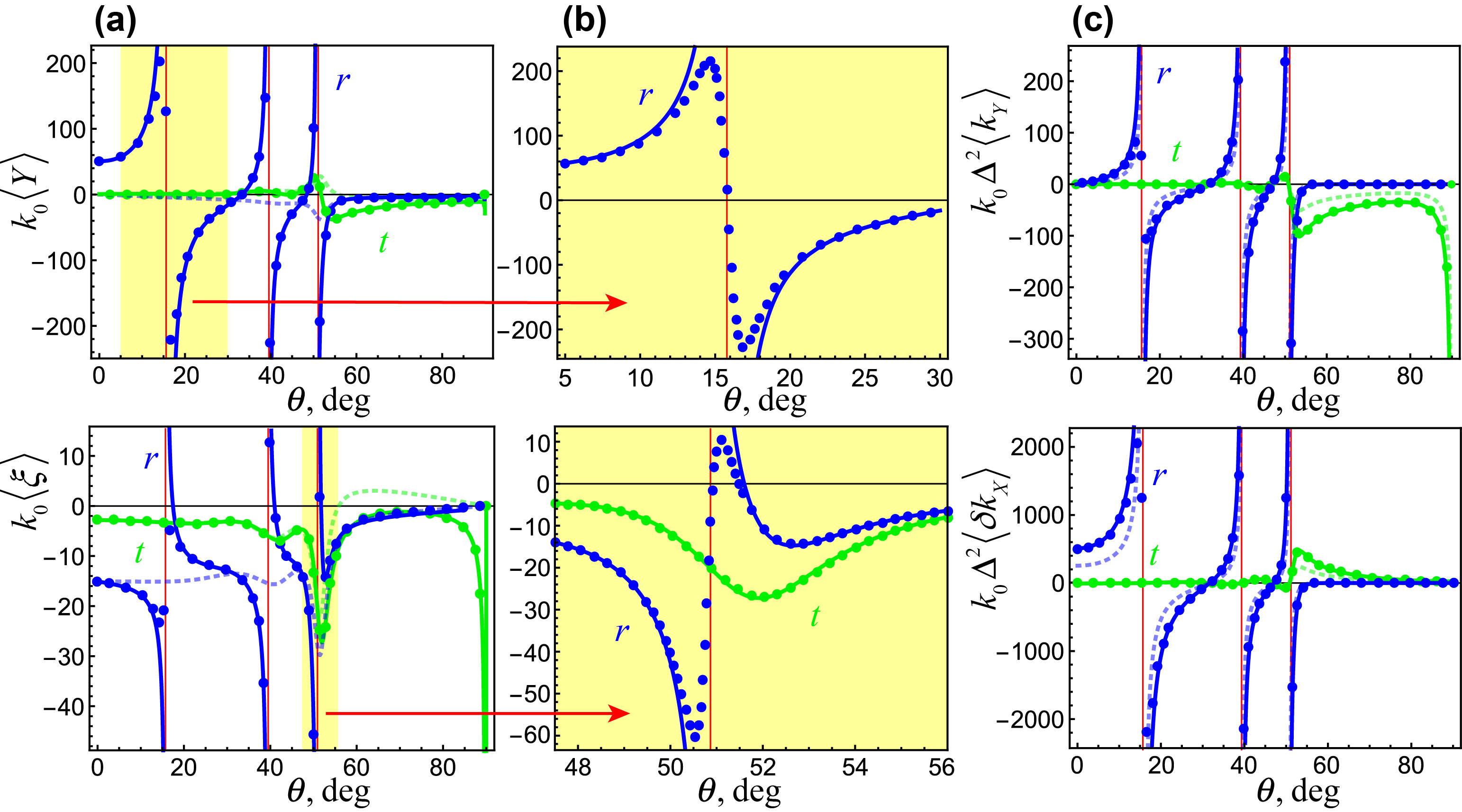
The resulting GH and Wigner shifts are given by sums of the corresponding Gaussian-packet shifts (7)–(10) and -dependent contributions (14)–(16). Figures 4–6 show these shifts for the vortex wavepacket with as functions of the angle of incidence in particular cases of barriers (A)–(C). In spite of the fact that the vortex-induced effects (14)–(16) are expressed via the Gaussian-packet shifts (7)–(10), the behaviour of the vortex-induced shifts and time differs dramatically. First, the vortex induced GH shifts and time delays of the scattered vortex wavepackets are present even for purely real scattering amplitudes [e.g., for in the step-potential case (A)], when the corresponding Gaussian-packet effects vanish. Second, the GH shifts of vortex wavepackets are generally non-zero at normal incidence . This is because the presence of a vortex breaks symmetry of the problem. Finally, the magnitude and sign of the vortex-induced shifts and time delays can be efficiently controlled by the vortex charge , i.e., a parameter of the incident wavepacket. This can have implementations in vortex-induced transport phenomena, such as Hall and Magnus effects. We also emphasize the resonant amplification of the GH shifts and Wigner time delays in the vicinity of critical incidence in the case (A) and transmission resonances (i.e., zeros of the reflection amplitude) in the case (C). Approximate analytical formulas (7)–(10) and (14)–(16) diverge near such singularities, whereas the shifts/delays can exceed their typical values by several orders of magnitude [43, 24, 45, 54, 56, 18, 55, 36].
4 Numerical calculations and additional corrections
4.1 Equations for numerical calculations
To check the above theoretical derivations, we performed numerical calculations of the reflection/transmission of a Laguerre-Gaussian vortex wavepacket by potential barriers (A)–(C) by applying exact boundary conditions and wavevector-dependent scattering amplitudes (2)–(4) to each plane wave in the incident wavepacket spectrum (11). This provides transformations of the wavefunctions in the momentum representation: and . In the paraxial approximation, the scattering amplitudes can be expanded in the Taylor series near the central wavevector:
| (17) |
These equations should be supplied with the corresponding transformations of each wavevector [10, 11, 12, 36]. Using the dispersion relations together with the conservation of the energy and -components of the momentum (wavevector) at interfaces, we derive the following relations between the deflections of the wavevectors from their central values:
| (18) |
Here , Eqs. (4.1) are derived in the second-order approximation in , and we introduced auxiliary quantities
| (19) |
The spatial and angular shifts are calculated as expectation values of the corresponding operators in the momentum representation:
| (20) |
where the inner product involves integration over the corresponding wavevector components . Substituting the wavefunctions and wavevector components of the scattered wavepackets, Eqs. (17)–(4.1) into Eqs. (4.1), we obtain the formalism for calculations of all of the required shifts. In doing so, all quantities are expressed via the parameters of the incident wavepacket. In particular, the derivatives with respect to the wavevector components in the first two Eqs. (4.1) are expressed, using relations (4.1) and (4.1), as
| (21) |
Importantly, for reflected wavepackets and transmitted wavepackets with , i.e., in all cases apart from the refraction at the step potential, case (A), the coefficients (4.1) vanish: . In such case, Eqs. (4.1) and (4.1) are simplified dramatically and become equivalent to standard equation for optical beams [10, 11, 12, 36]. The results of numerical calculations of Eqs. (17)–(4.1) with are depicted by symbols in Figs. 4–6. One can see that they perfectly agree with the analytical expressions (7)–(10) and (14)–(16) everywhere apart from the vicinity of resonant singularities. Analytical description of the resonant behaviour of wavepacket shifts, which regularizes divergencies of the Artmann and Wigner formulas, can be constructed within the nonlinear quantum-weak-weasurement approach [52, 18].
4.2 Additional corrections for the refraction at a step potential
The nontrivial case of the transmitted wavepacket at a step potential, case (A), when the coefficients (4.1) do not vanish, requires additional considerations. We have shown that calculations without the , , , terms in Eqs. (4.1) and (4.1) yield the shifts described by equations (7)–(10) and (14)–(16). Hence, substituting the , , , terms of Eqs. (4.1) and (4.1) into Eqs. (4.1), we obtain corrections to the results of previous sections. For angular shifts, this yields
| (22) |
| (23) |
For linear shifts, we obtain
| (24) |
| (25) |
Remarkably the , , corrections in Eqs. (22)–(25) affect even the shifts of Gaussian wavepackets, . Thus, that the standard Artmann and Wigner formulae (7)–(10) become inaccurate in the case of the refraction at a step potential.
Figure 7 shows the linear and angular shifts of transmitted wavepackets at a step potential, both analytical expressions (22)–(25) and numerical calculations using Eqs. (17)–(4.1). By comparing these plots with Fig. 4 one can see that the , , , corrections can considerably modify the values of the shifts and even change their signs.
5 Concluding remarks
We have described reflection and transmission of a localized 2D quantum vortex wavepacket at a planar potential barrier. We considered elliptical Laguerre-Gaussian-type wavepackets and step-like, delta-function, and rectangular potentials. Employing the analogy with the previously analysed reflection/refraction of optical vortex beams and spatiotemporal pulses, we have derived analytical expressions for the GH shifts and Wigner time delays of the reflected and transmitted wavepackets. In doing so, both ‘linear’ (space-time) and ‘angular’ (wavevector-energy) shifts were calculated. (The angular shifts have been mostly ignored so far in quantum problems.)
Importantly, the presence of a vortex dramatically modifies these shifts, previously known only for Gaussian-type wavepackets. First, the vortex-modified linear shifts and time delays appear even for purely real scattering coefficients, where the standard Artmann and Wigner expressions vanish. Second, the GH shifts of vortex wavepackets are generally non-zero even at normal incidence. Finally, the magnitudes and signs of all the vortex-induced shifts can be controlled by the topological charge of the vortex, . Furthermore, we have shown that the shifts and time delays can be resonantly enhanced by several orders of magnitude near the critical angle of incidence for a step potential and near zeros of the reflection amplitude (transmission resonances) for a rectangular barrier.
In addition to the analytical expressions, we have performed numerical calculations of the GH and Wigner shifts using the Fourier plane-wave expansions of the incident and scattered wavepackets. One can expect that the new shifts and time delays described in our work can manifest themselves in vortex-dependent transport phenomena in 2D quantum systems, including superfluids, quantum-Hall systems, 2D electron gas, ferromagnets, etc. While here we considered scattering of a vortex wavepacket by a planar scalar potential, it is worth mentioning that another lateral shift phenomenon appears upon scattering of a Gaussian wavepacket by a vortex Aharonov-Bohm vector-potential [57, 58]. This phenomenon also owes its origin to the fine interference of plane waves in the scattered wavepacket.
Acknowledgements
We are grateful to Professor M. V. Berry for providing an ongoing inspiration to play with waves, phases, currents, and singularities. This work is dedicated to him on the occasion of his 80th birthday.
References
References
- [1] Nye J F and Berry M V 1974 \titlecapDislocations in wave trains Proc. R. Soc. Lond. Ser. A 336 165–190
- [2] Berry M V 1981 Singularities in Waves Les Houches Lecture Series Session XXXV ed Balian R, Kleman M and Poirier J P (North-Holland: Amsterdam) pp 453–543
- [3] Rubinsztein-Dunlop H, Forbes A, Berry M V, Dennis M R, Andrews D L, Mansuripur M, Denz C, Alpmann C, Banzer P, Bauer T, Karimi E, Marrucci L, Padgett M, Ritsch-Marte M, Litchinitser N M, Bigelow N P, Rosales-Guzmán C, Belmonte A, Torres J P, Neely T W, Baker M, Gordon R, Stilgoe A B, Romero J, White A G, Fickler R, Willner A E, Xie G, McMorran B and Weiner A M 2016 \titlecapRoadmap on structured light J. Opt. 19 013001
- [4] Aharonov Y, Albert D Z and Vaidman L 1988 \titlecapHow the result of a measurement of a component of the spin of a spin-1/2 particle can turn out to be 100 Phys. Rev. Lett. 60 1351–1354
- [5] Berry M, Zheludev N, Aharonov Y, Colombo F, Sabadini I, Struppa D C, Tollaksen J, Rogers E T F, Qin F, Hong M, Luo X, Remez R, Arie A, Götte J B, Dennis M R, Wong A M H, Eleftheriades G V, Eliezer Y, Bahabad A, Chen G, Wen Z, Liang G, Hao C, Qiu C W, Kempf A, Katzav E and Schwartz M 2019 \titlecapRoadmap on superoscillations J. Opt. 21 053002
- [6] Dressel J, Malik M, Miatto F M, Jordan A N and Boyd R W 2014 \titlecapColloquium: Understanding quantum weak values: Basics and applications Rev. Mod. Phys. 86 307–316
- [7] Chiao R Y and Steinberg A M 1997 \titlecapTunneling times and superluminality Prog. Opt. 37 345–405
- [8] de Carvalho C A A and Nussenzveig H M 2002 \titlecapTime delay Phys. Rep. 364 83–174
- [9] Winful H G 2006 \titlecapTunneling time, the Hartman effect, and superluminality: A proposed resolution of an old paradox Phys. Rep. 436 1–69
- [10] Bliokh K Y and Aiello A 2013 \titlecapGoos-Hänchen and Imbert-Fedorov beam shifts: an overview J. Opt. 15 014001
- [11] Götte J B and Dennis M R 2012 \titlecapGeneralized shifts and weak values for polarization components of reflected light beams New J. Phys. 14 073016
- [12] Töppel F, Ornigotti M and Aiello A 2013 \titlecapGoos-Hänchen and Imbert-Fedorov shifts from a quantum-mechanical perspective New J. Phys. 15 113059
- [13] Bliokh K Y, Rodríguez-Fortuño F J, Nori F and Zayats A V 2015 \titlecapSpin-orbit interactions of light Nat. Photon. 9 796–808
- [14] Xiao S, Wang J, Liu F, Zhang S, Yin X and Li J 2017 \titlecapSpin-dependent optics with metasurfaces Nanophotonics 6 215–234
- [15] Hosten O and Kwiat P 2008 \titlecapObservation of the Spin Hall Effect of Light via Weak Measurements Science 319 787–790
- [16] Berry M V 2009 \titlecapOptical currents J. Opt. A: Pure Appl. Opt. 11 094001
- [17] Bliokh K Y, Bekshaev A Y, Kofman A G and Nori F 2013 \titlecapPhoton trajectories, anomalous velocities and weak measurements: a classical interpretation New J. Phys. 15 073022
- [18] Asano M, Bliokh K Y, Bliokh Y P, Kofman A G, Ikuta R, Yamamoto T, Kivshar Y S, Yang L, Özdemir N I S K and Nori F 2016 \titlecapAnomalous time delays and quantum weak measurements in optical micro-resonators Nat. Commun. 7 13488
- [19] Dragoman D and Dragoman M 2004 Quantum-Classical Analogies (Springer)
- [20] Wigner E P 1954 \titlecapLower Limit for the Energy Derivative of the Scattering Phase Shift Phys. Rev. 98 145–147
- [21] Goos F and Hänchen H 1947 \titlecapEin neuer und fundamentaler Versuch zur Totalreflexion Ann. Phys. 1 333–346
- [22] Artmann K 1948 \titlecapBerechnung der Seitenversetzung des totalreflektierten Strahles Ann. Phys. 2 87–102
- [23] Fedoseyev V G 2001 \titlecapSpin-independent transverse shift of the centre of gravity of a reflected and of a refracted light beam Opt. Commun. 193 9–18
- [24] Dasgupta R and Gupta P K 2006 \titlecapExperimental observation of spin-independent transverse shift of the centre of gravity of a reflected Laguerre-Gaussian light beam Opt. Commun. 257 91–96
- [25] Fedoseyev V G 2008 \titlecapTransformation of the orbital angular momentum at the reflection and transmission of a light beam on a plane interface J. Phys. A: Math. Theor. 41 505202
- [26] Bliokh K Y, Shadrivov I V and Kivshar Y S 2009 \titlecapGoos-Hänchen and Imbert-Fedorov shifts of polarized vortex beams Opt. Lett. 34 389–391
- [27] Merano M, Hermosa N, Woerdman J P and Aiello A 2010 \titlecapHow orbital angular momentum affects beam shifts in optical reflection Phys. Rev. A 82 023817
- [28] Dennis M R and Götte J B 2012 \titlecapTopological Aberration of Optical Vortex Beams: Determining Dielectric Interfaces by Optical Singularity Shifts Phys. Rev. Lett. 109 183903
- [29] Bliokh K Y and Nori F 2012 \titlecapSpatiotemporal vortex beams and angular momentum Phys. Rev. A 86 033824
- [30] Jhajj N, Larkin I, Rosenthal E W, Zahedpour S, Wahlstrand J K and Milchberg H M 2016 \titlecapSpatiotemporal Optical Vortices Phys. Rev. X 6 031037
- [31] Hancock S W, Zahedpour S, Goffin A and Milchberg H M 2019 \titlecapFree-space propagation of spatiotemporal optical vortices Optica 6 1547
- [32] Chong A, Wan C, Chen J and Zhan Q 2020 \titlecapGeneration of spatiotemporal optical vortices with controllable transverse orbital angular momentum Nat. Photon. 14 350
- [33] Bliokh K Y 2021 \titlecapSpatiotemporal Vortex Pulses: Angular Momenta and Spin-Orbit Interaction Phys. Rev. Lett. 126 243601
- [34] Zang Y, Mirando A and Chong A 2022 \titlecapSpatiotemporal optical vortices with arbitrary orbital angular momentum orientation by astigmatic mode converters Nanophotonics 11 745–752
- [35] Huang J, Zhang J, Zhu T and Ruan Z 2022 \titlecapSpatiotemporal Differentiators Generating Optical Vortices with Transverse Orbital Angular Momentum and Detecting Sharp Change of Pulse Envelope Laser Photonics Rev. 2100357
- [36] Mazanov M, Sugic D, Alonso M A, Nori F and Bliokh K Y 2021 \titlecapTransverse shifts and time delays of spatiotemporal vortex pulses reflected and refracted at a planar interface Nanophotonics 20210294
- [37] Huebener R P, Schopohl N and Volovik G E (eds) 2002 Vortices in Unconventional Superconductors and Superfluids (Springer)
- [38] Fetter A L 2009 \titlecapRotating trapped Bose-Einstein condensates Rev. Mod. Phys. 81 647–691
- [39] Nagaosa N and Tokura Y 2013 \titlecapTopological properties and dynamics of magnetic skyrmions Nature Nanotechnology 8 899–911
- [40] Thouless D J, Ao P and Niu Q 1996 \titlecapTransverse Force on a Quantized Vortex in a Superfluid Phys. Rev. Lett. 76 3758–3761
- [41] Stone M 1996 \titlecapMagnus force on skyrmions in ferromagnets and quantum Hall systems Phys. Rev. B 53 16573–16578
- [42] Thaller B 2000 Visual Quantum Mechanics (Springer, Berlin)
- [43] Chan C C and Tamir T 1985 \titlecapAngular shift of a Gaussian beam reflected near the Brewster angle Opt. Lett. 10 378–380
- [44] Aiello A and Woerdman J P 2008 \titlecapRole of beam propagation in Goos-Hänchen and Imbert-Fedorov shifts Opt. Lett. 33 1437–1439
- [45] Merano M, Aiello A, van Exter M P and Woerdman J P 2009 \titlecapObserving angular deviations in the specular reflection of a light beam Nat. Photon. 3 337–340
- [46] Beenakker C W J, Sepkhanov R A, Akhmerov A R and Tworzydło J 2009 \titlecapQuantum Goos-Hänchen Effect in Graphene Phys. Rev. Lett. 102 146804
- [47] de Haan V O, Plomp J, Rekveldt T M, Kraan W H, van Well A A, Dalgliesh R M and Langridge S 2010 \titlecapObservation of the Goos-Hänchen Shift with Neutrons Phys. Rev. Lett. 104 010401
- [48] Wu Z, Zhai F, Peeters F M, Xu H Q and Chang K 2011 \titlecapValley-Dependent Brewster Angles and Goos-Hänchen Effect in Strained Graphene Phys. Rev. Lett. 106 176802
- [49] Chen X, Lu X J, Ban Y and Li C F 2013 \titlecapElectronic analogy of the Goos–Hänchen effect: a review J. Opt. 15 033001
- [50] Kogelnik H and Weber H P 1974 \titlecapRays, stored energy, and power flow in dielectric waveguides J. Opt. Soc. Am. 64 174–185
- [51] Balcou P and Dutriaux L 1997 \titlecapDual Optical Tunneling Times in Frustrated Total Internal Reflection Phys. Rev. Lett. 78 851–854
- [52] Gorodetski Y, Bliokh K Y, Stein B, Genet C, Shitrit N, Kleiner V, Hasman E and Ebbesen T W 2012 \titlecapWeak Measurements of Light Chirality with a Plasmonic Slit Phys. Rev. Lett. 109 013901
- [53] Jozsa R 2007 \titlecapComplex weak values in quantum measurement Phys. Rev. A 76 044103
- [54] Berry M V 2011 \titlecapLateral and transverse shifts in reflected dipole radiation Proc. R. Soc. A 467 2500–2519
- [55] del Hougne P, Yeo K B, Besnier P and Davy M 2021 \titlecapOn-Demand Coherent Perfect Absorption in Complex Scattering Systems: Time Delay Divergence and Enhanced Sensitivity to Perturbations Laser Photonics Rev. 15 2000471
- [56] Götte J B and Dennis M R 2013 \titlecapLimits to superweak amplification of beam shifts Opt. Lett. 38 2295–2297
- [57] Shelankov A L 1998 \titlecapMagnetic force exerted by the Aharonov-Bohm line Europhys. Lett. (EPL) 43 623–628
- [58] Berry M V 1999 \titlecapAharonov-Bohm beam deflection: Shelankov's formula, exact solution, asymptotics and an optical analogue J. Phys. A: Math. Gen. 32 5627–5641