Windowed total variation denoising and noise variance monitoring

The update of the restored signal and $\Lambda^{\circ}$ need to consider the sliding of index from $w^{m}_{i}$ to $w^{m}_{i+1}$: a restored signal point is unchanged under the influence of slide movement means $\hat{u}_{i-1}=u^{*}_{i}$. In [3], we have shown the following theorem:

The diffusion from the “new” sample $y_{i+m}$ changes only the last part of the restoration of $w^{i}_{m}$ up to the junction of two segments whose sign of the variation $v^{*}_{j-1}(\lambda)-v^{*}_{j}(\lambda)$ corresponds to that of $v^{*}_{K^{*}}(\lambda)-y_{n+1}$. We can establish a similar theorem (c.f. Theorem 2) about the influence of the first sample $y_{i}$ for the sliding window $w^{m}_{i}$: the removing of $y_{i}$ changes only the first part of the restoration.

To sum up, for updating $u^{*}(\lambda)$ to $\hat{u}(\lambda)$, only the first part and the last part of $w^{m}_{i}$ are changed. We introduce the following definitions:

For a given $\lambda$ (noted $\hat{\lambda}$), the cutting set $\mathcal{N}(\hat{\lambda})$ is given by $\{\lambda^{\circ}>\hat{\lambda}\}$. In [3], we showed the points inside a segment of $u^{*}(\hat{\lambda})$ are merged for $\lambda\leq\hat{\lambda}$, and the value of $\lambda$ provoking the merge is independent to the points outside the segment. By introducing the virtual segment (c.f. Definition 2), the estimation of $\Lambda^{\circ}$ can be broken into some sub-problems for each virtual segment, shown in proposition 1. Combining with Theorem 1 and 2, the elements of $\{\lambda^{\circ}\leq\hat{\lambda}\}$ inside the isolated sequence are not influenced by the sliding movement.

Let $\Delta g^{\circ}=(\Delta g(\lambda^{\circ}_{1}),\Delta g(\lambda^{\circ}_{2}),\cdots,\Delta g(\lambda^{\circ}_{n-1}))$, we note $\Lambda^{\circ,i}$ and $\Delta g^{\circ,i}$, two vectors of size $m-1$, the result of $w^{m}_{i}$. The results after sliding ($\Lambda^{\circ,i+1}$ and $\Delta g^{\circ,i+1}$) based on $w^{m}_{i+1}$ can be obtained by updating $\Lambda^{\circ,i}$ and $\Delta g^{\circ,i}$. In this section, we will propose an adaptation of the online algorithm proposed in [3] to the sliding windows.

We will only talk about the online estimation of $\Lambda^{\circ,i+1}$ from $\Lambda^{\circ,i}$ in detail. By following, we note an application of Algorithm 1 in [3] to a given sequence of $\{y\}$ and $\{\tau\}$ as $\Lambda^{\circ}=\text{DP-TV}(\{y\},\{\tau\})$.

After choosing $\hat{\lambda}\geq 0$, called the cutting point, the restoration for $w^{m}_{i}$ is $u^{*}(\hat{\lambda})$. We note $p$ and $j^{*}_{p}$ respectively the last point and the last segment of the non left-isolated sequence of $u^{*}(\hat{\lambda})$, $l$ and $j^{*}_{l}$ respectively the first point and the first segment of the non right-isolated sequence of $u^{*}(\hat{\lambda})$. $\Lambda^{\circ,i+1}$ can be splitted into four parts: (1) Some elements of $\{\lambda^{\circ,i+1}>\hat{\lambda}\}$ are changed following Proposition 1; (2) The non left-isolated sequence $\{\lambda^{\circ,i}_{j}\leq\hat{\lambda}\}$ for $j\leq p$ is influenced by the removal of the first point $y_{i}$; (3) The non right-isolated sequence $\{\lambda^{\circ,i}_{j}\leq\hat{\lambda}\}$ for $j\geq l$ is influenced by the new point $y_{i+m}$; (4) All $\lambda^{\circ,i}_{j}\leq\hat{\lambda}$ remains the same for $p<j<l$.

We treat at first the unchanged part of $\Lambda^{\circ,i+1}$ : due to the sliding, we have $\lambda^{\circ,i+1}_{\{\lambda^{\circ,i+1}_{p,\cdots,l-2}\leq\hat{\lambda}\}}=\lambda^{\circ,i}_{\{\lambda^{\circ,n}_{p+1,\cdots,l-1}\leq\hat{\lambda}\}}$.

For the non right-isolated sequence, let $\epsilon_{\lambda}>0$, $\Lambda^{a}=\lambda^{\circ,i+1}_{\{\lambda^{\circ,i+1}_{l-1,\cdots,m}\leq\hat{\lambda}\}}$ can be estimated by $\text{DP-TV}(y^{+}_{a},\tau^{+}_{a})$ with the virtual segment:

• •

  $y^{+}_{a}=\{v^{*}_{j^{*}_{l}}(\hat{\lambda})-\frac{\hat{\lambda}+\epsilon_{\lambda}}{2\text{sign}(v_{j^{*}_{l}}-v_{j^{*}_{l}-1})},y_{\{l+i-1,\cdots,m+i\}}\}$

• •

  $\tau^{+}_{a}=\{1,\tau_{\{l+i-1,\cdots,m+i\}}\}$

For the non left-isolated sequence, $\Lambda^{b}=\lambda^{\circ,i+1}_{\{\lambda^{\circ,i+1}_{1,\cdots,p-1}\leq\hat{\lambda}\}}$ can be estimated by $\text{DP-TV}(y^{+}_{b},\tau^{+}_{b})$ with the virtual segment:

• •

  $y^{+}_{b}=\{y_{\{i+1,\cdots,i+p-1\}},v^{*}_{j^{*}_{p}}(\hat{\lambda})+\frac{\hat{\lambda}+\epsilon_{\lambda}}{2\text{sign}(v_{j^{*}_{p}+1}-v_{j^{*}_{p}})}\}$

• •

  $\tau^{+}_{b}=\{\tau_{\{i+1,\cdots,i+p-1\}},1\}$

The isolated and non-isolated sequences can be assembled in $\Lambda^{c}=\{\lambda^{c}_{1},\cdots,\lambda^{c}_{m}\}$ with $\lambda^{c}_{k}=\lambda^{a}_{k-l+3}$ for $k\geq l-1$, $\lambda^{c}_{k}=\lambda^{b}_{k}$ for $k\leq p-1$ and $\lambda^{c}_{k}=\lambda^{\circ,n}_{k-1}$ for $p<k-1<l$.

It remains $\{\lambda^{\circ,i+1}>\hat{\lambda}\}$. Let $d=\{\lambda^{\circ,i+1}>\hat{\lambda}\}=\{\lambda^{c}_{k}>\hat{\lambda}\}$ containing indeed all the last points of $\hat{u}(\hat{\lambda})$’s segments, we can get $\Lambda^{d}=\lambda^{\circ,i+1}_{d}=\text{DP-TV}(\hat{v}(\hat{\lambda}),\hat{\mathcal{T}}(\hat{\lambda}))$.

Finally, $\Lambda^{\circ,i+1}$ can be assembled in the following way:

with $\alpha\mathrel{\mathop{\mathchar 58\relax}}\mathbb{Z}\to\mathbb{Z}$ giving the index of $i$ in the vector $d$.

The algorithm adapted for the sliding window is gathered in Algorithm 1. With a nice choice of $\hat{\lambda}$, only a small part ($\Lambda^{a},\Lambda^{b},\Lambda^{d}$) of the window $w^{m}_{i+1}$ needs to be updated from $w^{m}_{i}$. The overall complexity for estimating the restoration in a window of size $m$ is in $O(m)$.

We propose a method to detect the shift of noise’s variance based on our restoration method. For an observed signal $y$ of size $n$, we take a sliding window of size $m$ with $m<n$. For each window $w_{i}^{m}=[i,i+m-1]$, we apply our denoising algorithm with the automatic choice of $\lambda$ on the sequence $(y_{i},\cdots,y_{i+m-1})$ and $(\tau_{i},\cdots,\tau_{i+m-1})$ for estimating the restored signal $u^{*}(\lambda_{ours})=(u^{*}_{1},\cdots,u^{*}_{m})$. The windowed restoration residual for $j=1,\cdots,m$ is given by $r_{j}=y_{j+i-1}-u^{*}_{j}(\lambda_{ours})$. The variance of the residual inside $w_{i}^{m}$ can be estimated by:

with the mean value of residual $\overline{r}_{i}=\frac{1}{m}\sum_{j=1}^{m}r_{j}$.

For the simulation, the realisation of noise is $\hat{\epsilon}_{j}=y_{j}-u_{net,j}$ with $u_{net}$ the original signal and $j=1,\cdots,n$. The estimation of noise variance inside $w_{i}^{m}$ is given by $(\hat{\sigma}_{i}^{m})^{2}=\frac{1}{m-1}\sum_{j=i}^{i+m-1}(\hat{\epsilon}_{j}-\overline{\hat{\epsilon}}_{i})^{2}$ with $\overline{\hat{\epsilon}}_{i}=\frac{1}{m}\sum_{j=i}^{i+m-1}\hat{\epsilon}_{j}$.

Since $u^{*}(\lambda_{ours})$ is a good restoration of $y$, $u^{*}(\lambda_{ours})$ is similar to $u_{net}$, which means that $\sigma_{i}^{m*}$ is close to $\hat{\sigma}_{i}^{m}$ inside each window $w^{m}_{i}$. The noise variance $\sigma_{i}^{m*}$ is not available for the real data, so we propose to detect the variance shift in using the residual standard deviation vector $\sigma^{m*}=(\sigma^{m*}_{1},\cdots,\sigma^{m*}_{n-m+1})$ with $\sigma^{m*}_{i}$ obtained by (5) inside $w^{m}_{i}$.

For estimating the noise variance in a window of size $m$, the complexity is in $O(m)$ with the online implementation of sliding windows, and the overall complexity for monitoring the variance of a signal of size $n$ is in $O((n-m)m)$.

For the variance monitoring, the method needs to estimate accurately the noise variance in the ideal case or capture the variation of noise variance in a more realistic case. We use the following criteria to evaluate the performance of variance monitoring:

• •

  Average bias: $\overline{\text{bias}}=\frac{1}{n-m+1}\sum_{i=1}^{n-m+1}(\hat{\sigma}^{m}_{i}-\sigma^{m*}_{i})$.

• •

  Ratio of $\hat{\sigma}^{m}$ variation explained:

  $$\text{RVE}=1-\frac{\sum_{i=1}^{n-m+1}(\hat{\sigma}^{m}_{i}-\overline{\text{bias}}-\sigma^{m*}_{i})^{2}}{\sum_{i=1}^{n-m+1}(\hat{\sigma}^{m}_{i}-\overline{\hat{\sigma}^{m}})^{2}}$$

  (6)

  where $\overline{\hat{\sigma}^{m}}=\frac{1}{n-m+1}\sum_{i=1}^{n-m+1}(\hat{\sigma}^{m}_{i})$. It is indeed the $R^{2}$ score between $\sigma^{m*}$ and $\hat{\sigma}^{m}$ after adjusting those two items to the same mean value. The range of RVE is between $0$ and $1$, and $\text{RVE}=1$ indicates our estimation explains perfectly the variation of $\sigma^{m*}$.

We compare our method with Median Absolute Deviation (MAD) following the proposition of [12] and [13] $\sigma=1.4826\ \text{median}(By-\text{median}(By))$ with $By=\sqrt{2}(y_{2}-y_{1},\cdots,y_{n}-y_{n-1})$.

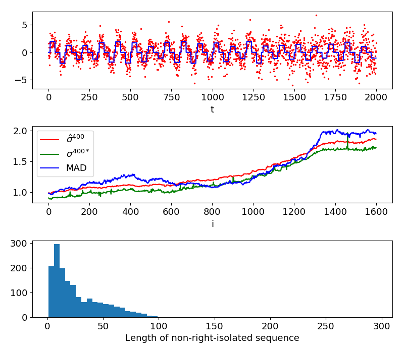
At first, we will fix the window length $m=400$. Our proposition requires a parameter $q$ which stands for the length of the approximation of derivative, see p13 in [3] for more details. We apply our method to a simulated piece-wise constant signal with the parameter $\log_{10}(q)=1$. An example of $y=u_{net}+\epsilon$ with $\epsilon\sim\mathcal{N}(0,\sigma_{a}^{2}(t))$ and the noise variance estimations for 400-point windows $w^{400}_{i}$ and $i=1,\cdots,1601$ are shown in Figure 1. Both MAD and our method propose an estimation similar to the variance of the noise realisation for every sliding windows. In this example, our method underestimates the variance, but the variation of our estimation inside each sliding window follows well that of $\hat{\sigma}^{400}$. The estimation of MAD propose a precise estimation, but does not follow the variation of $\hat{\sigma}^{400}$. The lengths of non-right-isolated sequence of each window (shown in Figure 1) are all smaller than the window size $m=400$, which means the influence of new sample remains inside each window and validates our assumption about the local influence.

We tested the performance of MAD and our approach under different noise hypothesis:

1. 1.

   $\mathcal{N}(0,\sigma_{a}^{2}(t))$ with $\sigma_{a}(t)=1+0.0005t$.

2. 2.

   $\mathcal{N}(0,\sigma_{b}^{2}(t))$ with $\sigma_{b}(t)=1$ for $t\leq 1000$ and $\sigma_{b}(t)=1+0.001t$ for $t>1000$.

3. 3.

   $\mathcal{U}(-d(t),d(t))$ with $d(t)=1+0.0005t$.

4. 4.

   $\mathcal{N}(0,\sigma_{a}^{2}(t))+\mathcal{U}(-1,1)$.

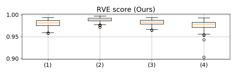
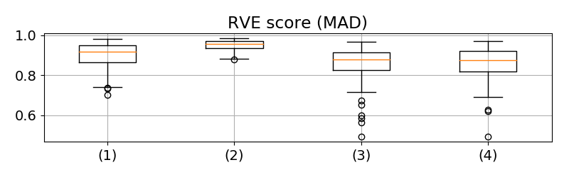
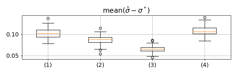
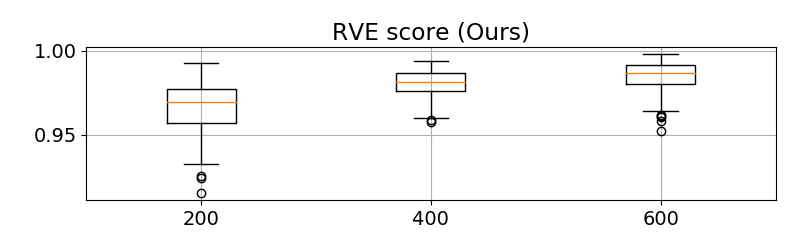
We have done 100 simulations for each type of noise, and the results are gathered in Figure 2. For the most of simulations, our method has $\text{RVE}>0.95$ and over-performs MAD. The high RVE score indicates the variation of our proposition fits well that of the real values, which allows us to monitor the variation of noise variance for the real signal collected from plants. However, the result of $\overline{\text{Bias}}$ shows our method always underestimates the noise variance, and the bias depends on the type of noise, which means we can not estimate an universal offset for removing this bias in a general case.

The windows length $m$ plays an important role in the restoration and the variance monitoring, and needs to be chosen carefully. A short window can capture the local variation of the noise variance, but the new point (i.e $(i+m)^{th}$ point) may still have a strong influence for the pass (i.e. $i-1,i-2,\cdots$), which limits the restoration performance for the pass points. We test $m=200,400,600$ with the noise $\epsilon\sim\mathcal{N}(0,\sigma^{2}_{a}(t))$, and the results are shown in Figure 3. A longer window provides a better performance of monitoring. But the local variation of $\sigma^{2}$ will be neglected for a long window, and the stationarity hypothesis inside the window is not validated anymore. The choice of $m$ is out of the scope of this article, and it remains an open question.

To sum up, our method can not provide a precise estimation of the noise’s variance values, but our estimation follows well that of the real value with an estimation error depending on the type of noise and the shape of original signal.

One of the applications of our method is to detect the shift of noise variance. The residual variance may stay stable (i.e $\sigma^{m*}_{i}=\sigma$) during the correct functional period, and the noise variance shift can be detected by a prefixed threshold over $\sigma^{m*}_{i}$ comparing to the stable regime: e.g $\sigma^{m*}_{i}>1.2\sigma$ for some successive sliding windows $w^{m}_{i}$.

References

- [1] L. I. Rudin, S. Osher, and E. Fatemi, “Nonlinear total variation based noise removal algorithms,” Physica D: nonlinear phenomena, 1992.
- [2] A. Chambolle and P.-L. Lions, “Image recovery via total variation minimization and related problems,” Numerische Mathematik, 1997.
- [3] Z. Liu, M. Perrodin, T. Chambrion, and R. Stoica, “Revisit 1d total variation restoration problem with new real-time algorithms for signal and hyper-parameter estimations,” arXiv preprint arXiv:2012.09481, 2020.
- [4] R. J. Tibshirani and J. Taylor, “The solution path of the generalized lasso,” The Annals of Statistics, 2011.
- [5] I. Pollak, A. S. Willsky, and Y. Huang, “Nonlinear evolution equations as fast and exact solvers of estimation problems,” IEEE Trans. on Signal Processing, 2005.
- [6] C. M. Stein, “Estimation of the mean of a multivariate normal distribution,” The annals of Statistics, 1981.
- [7] D.-H. Shin, R.-H. Park, S. Yang, and J.-H. Jung, “Block-based noise estimation using adaptive gaussian filtering,” IEEE Transactions on Consumer Electronics, 2005.
- [8] S. Beheshti and M. A. Dahleh, “A new information-theoretic approach to signal denoising and best basis selection,” IEEE Transactions on Signal Processing, 2005.
- [9] M. Hashemi and S. Beheshti, “Adaptive noise variance estimation in bayesshrink,” IEEE Signal Processing Letters, 2010.
- [10] J. Han and L. Xu, “A new method for variance estimation of white noise corrupting a signal,” in I2MTC, 2006.
- [11] S. Pyatykh, J. Hesser, and L. Zheng, “Image noise level estimation by principal component analysis,” IEEE transactions on image processing, 2012.
- [12] D. L. Donoho and J. M. Johnstone, “Ideal spatial adaptation by wavelet shrinkage,” biometrika, 1994.
- [13] S. Sardy and H. Monajemi, “Efficient threshold selection for multivariate total variation denoising,” Journal of Computational and Graphical Statistics, 2019.