Wireless Communication with Extremely Large-Scale Intelligent Reflecting Surface

\text{Chao~{}Feng}^{*}

\text{Haiquan~{}Lu}^{*}

\text{Yong~{}Zeng}^{*}\dagger

\text{Shi~{}Jin}^{*}

, and

\text{Rui~{}Zhang}^{\ddagger}

elezhang@nus.edu.sg *National Mobile Communications Research Laboratory, Southeast University, Nanjing 210096, China

\dagger

Purple Mountain Laboratories, Nanjing 211111, China

\ddagger

Department of Electrical and Computer Engineering, National University of Singapore, Singapore 117583
Email: needychao@gmail.com, {haiquanlu, yong_zeng, jinshi}@seu.edu.cn

Abstract

Intelligent reflecting surface (IRS) is a promising technology for wireless communications, thanks to its potential capability to engineer the radio environment. However, in practice, such an envisaged benefit is attainable only when the passive IRS is of a sufficiently large size, for which the conventional uniform plane wave (UPW)-based channel model may become inaccurate. In this paper, we pursue a new channel modelling and performance analysis for wireless communications with extremely large-scale IRS (XL-IRS). By taking into account the variations in signal’s amplitude and projected aperture across different reflecting elements, we derive both lower- and upper-bounds of the received signal-to-noise ratio (SNR) for the general uniform planar array (UPA)-based XL-IRS. Our results reveal that, instead of scaling quadratically with the increased number of reflecting elements $M$ as in the conventional UPW model, the SNR under the more practically applicable non-UPW model increases with $M$ only with a diminishing return and gets saturated eventually. To gain more insights, we further study the special case of uniform linear array (ULA)-based XL-IRS, for which a closed-form SNR expression in terms of the IRS size and transmitter/receiver location is derived. This result shows that the SNR mainly depends on the two geometric angles formed by the transmitter/receiver locations with the IRS, as well as the boundary points of the IRS. Numerical results validate our analysis and demonstrate the importance of proper channel modelling for wireless communications aided by XL-IRS.

I Introduction

Intelligent reflecting surface (IRS) is an emerging technology to achieve cost-effective and energy-efficient wireless communications by proactively reforming the radio propagation environment [1, 2, 3, 4, 5, 6, 7]. In a nutshell, IRS is a reconfigurable metasurface consisting of densely arranged low-cost passive elements and a smart controller. By adjusting the phase shift and/or amplitude of the incident signals on each reflecting element, the reflected signals can be added constructively or destructively at the desired or non-intended receivers, so as to achieve coverage enhancement, interference suppression, security enhancement, enhanced radio localization, etc [6, 7]. Moreover, IRS avoids costly radio frequency (RF) chains and operates in a full-duplex mode, which is thus free of self-interference and noise amplification. Besides IRS, several similar terminologies are also used in the literature, e.g., reconfigurable intelligent surface (RIS) [3, 5] and software controllable metasurface (SCS) [6, 8].

Despite of its great potentials, the promising performance gain brought by IRS is practically attainable only when the size of IRS is sufficiently large [9], so as to compensate for the double signal attenuation from the transmitter to IRS as well as from IRS to the receiver. Fortunately, the appealing features of IRS such as passive reflection without RF chains, lightweight and conformal geometry make it possible to deploy extremely large-scale IRSs (XL-IRSs) in the environment such as the facades of buildings, indoor walls and ceilings. However, the increased aperture of XL-IRS renders that the intended transmitter and/or receiver may not be located in the far-field region of the IRS, albeit that this generally holds for each of its reflecting elements due to their much smaller size (in the order of carrier wavelength) [10, 11]. As a result, the conventional uniform plane wave (UPW) model may become inaccurate for IRS channel modelling. In this case, the element-based approach should be adopted for more accurate IRS channel modelling and performance analysis, by considering the more practical spherical wavefront, the variations in signal’s amplitude and angles of arrival/departure (AoA/AoD) across different reflecting elements.

There have been some preliminary results on the mathematical modelling and performance analysis for wireless communications without assuming the conventional UPW model, most of which considered active arrays [11, 12, 13]. For example, in [11], by taking into account the variations in signal’s amplitude, phase and projected aperture over different array elements, a closed-form expression for the received signal-to-noise ratio (SNR) was derived for extremely large-scale array/surface communication, from which some useful insights were obtained. In [14], the power scaling laws and near-field behaviours of IRS were analyzed for the special case of two-dimensional (2D) channel modelling that only considered the azimuth AoA/AoD, instead of the more general three-dimensional (3D) modelling with both azimuth and elevation AoA/AoD.

In this paper, we study the 3D channel modelling and performance analysis for wireless communication with XL-IRS. By taking into account the variations in signal’s amplitude and projected aperture across reflecting elements, tight lower- and upper-bounds of the user received SNR are derived for the general uniform planar array (UPA)-based XL-IRS. Our results reveal that instead of scaling quadratically with the number of reflecting elements (denoted by $M$ ) as in the conventional UPW model [2, 7], the SNR under the more practical non-UPW model increases with $M$ only with a diminishing return and eventually gets saturated. To gain more insights, we further study the special case of uniform linear array (ULA)-based XL-IRS, for which a closed-form SNR expression in terms of the IRS size and transmitter/receiver location is derived. This result shows that the SNR mainly depends on the two geometric angles formed by the transmitter/receiver locations with the IRS, as well as the boundary points of the IRS. Numerical results are provided to validate our analysis and demonstrate the necessity of proper channel modelling for wireless communications aided by XL-IRS.

II System Model

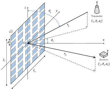
Refer to caption — Figure 1: Wireless communication with XL-IRS.

As shown in Fig. 1, we consider an IRS-aided communication system, where an XL-IRS is deployed to assist the communication between the transmitter and the receiver. Without loss of generality, the XL-IRS is assumed to be implemented by the sub-wavelength discrete UPA. The number of reflecting elements is denoted as $M\gg 1$ , and the separation between adjacent elements is $d\leq\frac{\lambda}{2}$ , with $\lambda$ denoting the signal wavelength. The physical size of each reflecting element is denoted as $\sqrt{A}\times\sqrt{A}$ , where $\sqrt{A}\leq d$ . We assume that IRS is placed on the $y$ - $z$ plane and centered at the origin, and $M=M_{y}M_{z}$ , where $M_{y}$ and $M_{z}$ denote the number of reflecting elements along the $y$ - and $z$ -axis, respectively. Therefore, the total physical size of the IRS is $L_{y}\times L_{z}$ , where $L_{y}\simeq M_{y}d$ and $L_{z}\simeq M_{z}d$ .

For notational convenience, $M_{y}$ and $M_{z}$ are assumed to be odd numbers. The central location of the $(m_{y},m_{z})$ th reflecting element is denoted as $\mathbf{w}_{m_{y},m_{z}}=[0,m_{y}d,m_{z}d]^{T}$ , where $m_{y}=0,\pm 1,\cdots,\pm(M_{y}-1)/2$ , $m_{z}=0,\pm 1,\cdots,\pm(M_{z}-1)/2$ . The transmitter location is denoted by $\mathbf{q}=[r_{q}\Psi_{q},r_{q}\Phi_{q},r_{q}\Omega_{q}]^{T}$ , with $\Psi_{q}\triangleq\sin\theta_{q}\cos\phi_{q}$ , $\Phi_{q}\triangleq\sin\theta_{q}\sin\phi_{q}$ , and $\Omega_{q}\triangleq\cos\theta_{q}$ , where $r_{q}$ is the distance between the transmitter and the center of the XL-IRS, and $\theta_{q}\in[0,\pi]$ and $\phi_{q}\in[-\frac{\pi}{2},\frac{\pi}{2}]$ denote the zenith and azimuth angles, respectively. The distance between the transmitter and the $(m_{y},m_{z})$ th reflecting element is

	$\displaystyle r_{q,m_{y},m_{z}}=\\|\mathbf{w}_{m_{y},m_{z}}-\mathbf{q}\\|$
	$\displaystyle\quad=r_{q}\sqrt{1-2m_{y}\varepsilon_{q}\Phi_{q}-2m_{z}\varepsilon_{q}\Omega_{q}+(m_{y}^{2}+m_{z}^{2})\varepsilon_{q}^{2}},$		(1)

where $\varepsilon_{q}\triangleq\frac{d}{r_{q}}$ . Since the element separation $d$ is on sub-wavelength scale, we have $\varepsilon_{q}\ll 1$ .

Similarly, denote the receiver location as $\mathbf{p}=[r_{p}\Psi_{p},r_{p}\Phi_{p},r_{p}\Omega_{p}]^{T}$ , with $\Psi_{p}\triangleq\sin\theta_{p}\cos\phi_{p}$ , $\Phi_{p}\triangleq\sin\theta_{p}\sin\phi_{p}$ , and $\Omega_{p}\triangleq\cos\theta_{p}$ , where $r_{p}$ is the distance between the receiver and the center of the XL-IRS, and $\theta_{p}\in[0,\pi]$ and $\phi_{p}\in[-\frac{\pi}{2},\frac{\pi}{2}]$ are the zenith and azimuth angles, respectively. The distance between the receiver and the $(m_{y},m_{z})$ th reflecting element is

r_{p,m_{y},m_{z}}=r_{p}\sqrt{1-2m_{y}\varepsilon_{p}\Phi_{p}-2m_{z}\varepsilon_{p}\Omega_{p}+(m_{y}^{2}+m_{z}^{2})\varepsilon_{p}^{2}},

(2)

where $\varepsilon_{p}\triangleq\frac{d}{r_{p}}\ll 1$ .

For ease of exposition, we assume that the transmitter and receiver each has one antenna and their direct link is negligible due to severe blockage. The links between the XL-IRS and the transmitter/receiver are dominated by the line-of-sight (LoS) path, by properly placing the IRS in practice. We focus on IRS implemented by using aperture reflecting element such as patch element, which is of low-profile and especially suitable to be mounted on a surface. For convenience, we assume that the aperture efficiency is unity so that the effective aperture of each element is equal to its physical area. By taking into account the variations in signal’s amplitude and projected aperture across different reflecting elements, the channel power gain between the transmitter and the $(m_{y},m_{z})$ th element of the XL-IRS can be modelled as [11]

	$\displaystyle a_{m_{y},m_{z}}(r_{q},\theta_{q},\phi_{q})=\underbrace{\frac{1}{4\pi r_{q,m_{y},m_{z}}^{2}}}_{\text{Free-space pathloss}}\underbrace{A\frac{(\mathbf{q}-\mathbf{w}_{m_{y},m_{z}})^{T}\hat{\mathbf{u}}_{x}}{\\|\mathbf{q}-\mathbf{w}_{m_{y},m_{z}}\\|}}_{\text{Projected aperture}}$
	$\displaystyle\quad=\frac{A\Psi_{q}}{4\pi r_{q}^{2}[1-2m_{y}\varepsilon_{q}\Phi_{q}-2m_{z}\varepsilon_{q}\Omega_{q}+(m_{y}^{2}+m_{z}^{2})\varepsilon_{q}^{2}]^{3/2}},$		(3)

where $\hat{\mathbf{u}}_{x}$ is a unit vector along the $x$ -axis, which is the normal vector of each IRS element. Similarly, the channel power gain between the receiver and the $(m_{y},m_{z})$ th element of the XL-IRS is

	$\displaystyle b_{m_{y},m_{z}}(r_{p},\theta_{p},\phi_{p})$
	$\displaystyle\quad=\frac{A\Psi_{p}}{4\pi r_{p}^{2}[1-2m_{y}\varepsilon_{p}\Phi_{p}-2m_{z}\varepsilon_{p}\Omega_{p}+(m_{y}^{2}+m_{z}^{2})\varepsilon_{p}^{2}]^{3/2}}.$		(4)

Denote the channel vector between the transmitter and the XL-IRS by $\mathbf{h}\in\mathbb{C}^{M\times 1}$ , whose elements are given by

h_{m_{y},m_{z}}=\sqrt{a_{m_{y},m_{z}}(r_{q},\theta_{q},\phi_{q})}e^{-j\frac{2\pi}{\lambda}r_{q,m_{y},m_{z}}},\forall m_{y},m_{z}.

(5)

Similarly, denote the channel vector between the XL-IRS and the receiver by $\mathbf{g}\in\mathbb{C}^{M\times 1}$ , with the elements given by

g_{m_{y},m_{z}}=\sqrt{b_{m_{y},m_{z}}(r_{p},\theta_{p},\phi_{p})}e^{-j\frac{2\pi}{\lambda}r_{p,m_{y},m_{z}}},\forall m_{y},m_{z}.

(6)

Further denote by $\theta_{m_{y},m_{z}}$ the phase shift introduced by the $(m_{y},m_{z})$ th reflecting element of the XL-IRS, and $\mathbf{\Theta}\in\mathbb{C}^{M\times M}$ is a diagonal phase shift matrix with the diagonal element given by $e^{j\theta_{m_{y},m_{z}}}$ . Then the received signal can be expressed as $y=\mathbf{g}^{T}\mathbf{\Theta}{\mathbf{h}}\sqrt{P}s+n$ , where $P$ and $s$ are the transmit power and information-bearing symbol, respectively, and $n\sim\mathcal{CN}(0,\sigma^{2})$ is the additive white Gaussian noise (AWGN) at the receiver.

With the optimal phase shifting by the XL-IRS, i.e., $\theta_{m_{y},m_{z}}=\frac{2\pi}{\lambda}r_{q,m_{y},m_{z}}+\frac{2\pi}{\lambda}r_{p,m_{y},m_{z}}$ , the maximum SNR at the receiver can be obtained as

\gamma=\bigg{(}\sum_{m_{y}=-\frac{M_{y}-1}{2}}^{\frac{M_{y}-1}{2}}\sum_{m_{z}=-\frac{M_{z}-1}{2}}^{\frac{M_{z}-1}{2}}|h_{m_{y},m_{z}}||g_{m_{y},m_{z}}|\bigg{)}^{2}\bar{P},

(7)

where $\bar{P}\triangleq\frac{P}{\sigma^{2}}$ .

III Performance Analysis

		$\displaystyle\gamma=\frac{A^{2}\bar{P}\Psi_{q}\Psi_{p}}{16\pi^{2}r_{q}^{2}r_{p}^{2}}$		(8)
		$\displaystyle\times\bigg{\|}\sum_{m_{z}=-\frac{M_{z}-1}{2}}^{\frac{M_{z}-1}{2}}\sum_{m_{y}=-\frac{M_{y}-1}{2}}^{\frac{M_{y}-1}{2}}\frac{1}{[1-2m_{y}\varepsilon_{q}\Phi_{q}-2m_{z}\varepsilon_{q}\Omega_{q}+(m_{y}^{2}+m_{z}^{2})\varepsilon_{q}^{2}]^{3/4}[1-2m_{y}\varepsilon_{p}\Phi_{p}-2m_{z}\varepsilon_{p}\Omega_{p}+(m_{y}^{2}+m_{z}^{2})\varepsilon_{p}^{2}]^{3/4}}\bigg{\|}^{2}$		(8)

\displaystyle\gamma\simeq\frac{A^{2}\bar{P}\Psi_{q}\Psi_{p}}{16\pi^{2}d^{4}r_{q}^{2}r_{p}^{2}}\bigg{|}\int_{-\frac{L_{z}}{2}}^{\frac{L_{z}}{2}}\int_{-\frac{L_{y}}{2}}^{\frac{L_{y}}{2}}\frac{\mathrm{d}y\mathrm{d}z}{[1-\frac{2}{r_{q}}y\Phi_{q}-\frac{2}{r_{q}}z\Omega_{q}+\frac{1}{r_{q}^{2}}(y^{2}+z^{2})]^{3/4}[1-\frac{2}{r_{p}}y\Phi_{p}-\frac{2}{r_{p}}z\Omega_{p}+\frac{1}{r_{p}^{2}}(y^{2}+z^{2})]^{3/4}}\bigg{|}^{2}

(9)

In this section, performance analysis is carried out based on the SNR expression in (7). By substituting (1)-(6) into (7), the resulting SNR can be written as (LABEL:8), shown at the top of the next page. Furthermore, by following similar techniques as [11] and using the fact that $\varepsilon_{q}\ll 1$ and $\varepsilon_{p}\ll 1$ , the double summation in (LABEL:8) can be approximated by the corresponding double integral. As a result, the SNR can be expressed in an integral form given in (9), shown at the top of the next page.

III-A SNR Lower- and Upper-Bounds

Theorem 1

For the communication aided by an XL-IRS, the SNR in (9) is lower-/upper-bounded by

f(R_{1})\leq\gamma\leq f(R_{2}),

(8)

where the function $f(R)$ is defined as (11) shown at the top of the next page, and $R_{1}=\frac{1}{2}\mathrm{min}\{L_{y},L_{z}\}$ , $R_{2}=\frac{1}{2}\sqrt{L_{y}^{2}+L_{z}^{2}}$ .

\displaystyle f(R)\triangleq\frac{A^{2}\bar{P}\Psi_{q}\Psi_{p}}{16\pi^{2}d^{4}r_{q}^{2}r_{p}^{2}}\bigg{|}\int_{0}^{2\pi}\mathrm{d}\zeta\int_{0}^{R}\frac{r\mathrm{d}r}{(1-\frac{2r}{r_{q}}\Phi_{q}\cos\zeta-\frac{2r}{r_{q}}\Omega_{q}\sin\zeta+\frac{r^{2}}{r_{q}^{2}})^{3/4}(1-\frac{2r}{r_{p}}\Phi_{p}\cos\zeta-\frac{2r}{r_{p}}\Omega_{p}\sin\zeta+\frac{r^{2}}{r_{p}^{2}})^{3/4}}\bigg{|}^{2}

(11)

Proof:

Theorem 1 can be shown by noting that the SNR in (9) is given by an integral over the rectangular region $L_{y}\times L_{z}$ occupied by the XL-IRS. By replacing this rectangular region with its inscribed disk and circumscribed disk that have radii $R_{1}$ and $R_{2}$ , respectively, lower- and upper-bounds in (8) can be obtained as an integral in polar coordinate after a change of variables. ∎

For convenience, we define the distance ratio as $\rho\triangleq r_{q}/r_{p}$ . Without loss of generality, we may assume that $0<\rho\leq 1$ due to symmetry.

Lemma 1

If the transmitter and receiver are both located along the boresight of the XL-IRS, i.e., near the $x$ -axis with $\Phi_{q},\Phi_{p}\ll\frac{r_{q}}{L_{y}}$ and $\Omega_{q},\Omega_{p}\ll\frac{r_{q}}{L_{z}}$ , we have

\begin{cases}\frac{\rho}{1-\rho^{2}}\xi^{2}\bar{P}G(R_{1})\leq\gamma\leq\frac{\rho}{1-\rho^{2}}\xi^{2}\bar{P}G(R_{2}),&0<\rho<1\\ \\ \gamma=\frac{\xi^{2}\bar{P}}{\pi^{2}}\arctan^{2}\frac{(\frac{L_{y}}{2r_{q}})(\frac{L_{z}}{2r_{q}})}{\sqrt{(\frac{L_{y}}{2r_{q}})^{2}+(\frac{L_{z}}{2r_{q}})^{2}+1}},&\rho=1\end{cases}

(9)

where $\xi\triangleq\frac{A}{d^{2}}$ with $\rho<1$ is the array occupation ratio [11], and the function $G(R)$ is defined as

	$\displaystyle G(R)$	$\displaystyle\triangleq\bigg{[}F(\frac{1}{2}\arctan\frac{\sqrt{1-\rho^{2}}}{\rho}\|2)$
		$\displaystyle-F(\frac{1}{2}\arctan(\frac{\sqrt{1-\rho^{2}}}{\rho}\cos(\arctan\frac{R}{r_{q}}))\|2)\bigg{]}^{2},$		(10)

and $F(\vartheta|k)=\int_{0}^{\vartheta}\frac{1}{\sqrt{1-k\sin^{2}\beta}}\mathrm{d}\beta$ is the incomplete Elliptic Integral of the First Kind [15].

Proof:

Please refer to Appendix A. ∎

Lemma 2

Under the same condition as Lemma 1, the asymptotic SNR aided by the XL-IRS is

\displaystyle\lim_{L_{y},L_{z}\rightarrow\infty}\gamma=\begin{cases}\frac{\rho}{1-\rho^{2}}\xi^{2}\bar{P}\bigg{[}F(\frac{1}{2}\arctan\frac{\sqrt{1-\rho^{2}}}{\rho}|2)\bigg{]}^{2},&0<\rho<1\\ \\ \frac{\xi^{2}\bar{P}}{\pi^{2}}\times(\frac{\pi}{2})^{2}=\frac{\xi^{2}\bar{P}}{4},&\rho=1\end{cases}

(11)

Proof:

For $0<\rho<1$ , as $L_{y},L_{z}\rightarrow\infty$ , the radii of the inscribed disk and the circumscribed disk also go to infinity, i.e., $R_{1},R_{2}\rightarrow\infty$ . It then follows from (9) and (10) that both lower- and upper-bounds of the SNR approach to the same value. Therefore, the first case of (11) follows according to the Squeeze Theorem [16]. Besides, for $\rho=1$ , the resulting SNR can be easily obtained by letting $L_{y},L_{z}\rightarrow\infty$ in the second case of (9). ∎

As a comparison, the SNR under the commonly used UPW model for the same system setup is given by [1, 7]

\gamma_{UPW}=\frac{\beta_{0}^{2}\bar{P}}{r_{q}^{2}r_{p}^{2}}M^{2},

(12)

where $\beta_{0}$ is the channel gain at the reference distance of $1\,$ m. The result (12) is known as the square power scaling law for IRS-assisted communication, which is valid when both $r_{q}$ and $r_{p}$ are sufficiently large as compared to the IRS dimension (i.e., $M$ is moderately large), under which the far-field propagation model holds for both the whole IRS as well as each of its individual elements. However, if $M$ goes even larger, the above result cannot hold anymore as the square power scaling law implies that the SNR would increase unboundedly, which is obviously impractical. In contrast, our new result in Lemma 2 reveals that under the practical non-UPW model, the SNR will increase with $M$ , but with a diminishing return, and eventually approach to a constant that only depends on the distance ratio $\rho$ , and the array occupation ratio $\xi$ .

\displaystyle\gamma\simeq\frac{A^{2}\bar{P}\Psi_{q}\Psi_{p}}{16\pi^{2}d^{2}r_{q}^{2}r_{p}^{2}}\bigg{|}\int_{-\frac{L_{z}}{2}}^{\frac{L_{z}}{2}}\frac{\mathrm{d}z}{[(1-\frac{2}{r_{q}}z\cos\theta_{q}+\frac{z^{2}}{r_{q}^{2}})(1-\frac{2}{r_{p}}z\cos\theta_{p}+\frac{z^{2}}{r_{p}^{2}})]^{3/4}}\bigg{|}^{2}

(16)

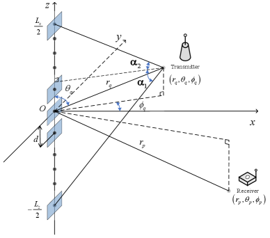
III-B ULA-based XL-IRS

To gain more insights, we consider the special case of ULA-based XL-IRS, where $M_{y}=1$ and $M_{z}=M$ . In this case, by letting $y=0$ and $\mathrm{d}y=d$ , the SNR expression in (9) reduces to (16) shown at the top of the next page.

Lemma 3

For the communication aided by a ULA-based XL-IRS, when $r_{q}\ll r_{p}$ (i.e., $\rho\rightarrow 0$ ), the SNR in (16) can be expressed as

\gamma=\frac{A^{2}\bar{P}\Psi_{p}\cos\phi_{q}}{4\pi^{2}d^{2}r_{p}^{2}}\bigg{[}F(\frac{\alpha_{1}}{2}|2)+F(\frac{\alpha_{2}}{2}|2)\bigg{]}^{2},

(13)

where $\alpha_{1}=\arctan\frac{L_{z}/2+r_{q}\cos\theta_{q}}{r_{q}\sin\theta_{q}}$ and $\alpha_{2}=\arctan\frac{L_{z}/2-r_{q}\cos\theta_{q}}{r_{q}\sin\theta_{q}}$ .

Proof:

Please refer to Appendix B. ∎

Note that the condition $r_{q}\ll r_{p}$ in Lemma 3 corresponds to the typical IRS deployment scenario, where it has been shown that IRS should be deployed closer to either the transmitter or receiver for SNR maximization [1, 7]. Lemma 3 shows that with a ULA-based XL-IRS, the IRS size $L_{z}$ affects the SNR via the two geometric angles, $\alpha_{1}$ and $\alpha_{2}$ , which are the angles formed by the line segments connecting the transmitter location and its projection to the IRS, as well as the two ends of the IRS, as shown in Fig. 2. In particular, $\alpha_{1}+\alpha_{2}$ is termed as the angular span [10]. It is not difficult to see that both $\alpha_{1}$ and $\alpha_{2}$ increase with the IRS size $L_{z}$ and decrease with the distance $r_{q}$ . Since the Elliptic Integral function $F(\vartheta|2)$ monotonically increases with $\vartheta$ , the SNR $\gamma$ in (13) increases with $L_{z}$ but decreases with $r_{q}$ , as expected. Furthermore, different from the conventional square power scaling law obtained based on the UPW model where the SNR increases unboundedly with the IRS size [2, 7], Lemma 3 shows that under the non-UPW model, the SNR increases with $L_{z}$ with a diminishing return. In particular, as $L_{z}\rightarrow\infty$ , we have $\alpha_{1}=\alpha_{2}=\frac{\pi}{2}$ , which leads to the following result.

Lemma 4

Under the same condition as Lemma 3, the asymptotic SNR in the case of ULA-based XL-IRS is

	$\displaystyle\lim_{L_{z}\rightarrow\infty}\gamma$	$\displaystyle=\frac{A^{2}\bar{P}\Psi_{p}\cos\phi_{q}}{\pi^{2}d^{2}r_{p}^{2}}\bigg{[}F(\frac{\pi}{4}\|2)\bigg{]}^{2}$
		$\displaystyle=1.7188\times\frac{A^{2}\bar{P}\Psi_{p}}{\pi^{2}d^{2}r_{p}^{2}}\cos\phi_{q}.$		(14)

IV Numerical Results

In this section, numerical results are provided to validate our theoretical analysis, and also compare our proposed model with the conventional UPW model. Unless otherwise stated, the signal wavelength is $\lambda=0.125\,$ m, the element seperation is set as $d=\frac{\lambda}{5}$ , and the element size is $A=(\frac{d}{2})^{2}$ , which corresponds to the array occupation ratio $\xi=\frac{1}{4}$ .

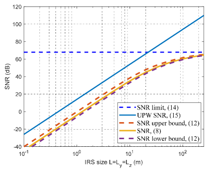
Fig. 3 plots the SNR versus IRS size for square UPA-based XL-IRS, i.e., $L=L_{y}=L_{z}$ . The results based on the summation in (LABEL:8), closed-form lower- and upper-bounds in (9), the asymptotic value in (11), and that under the conventional UPW model in (12) are compared. The transmit SNR is $\bar{P}=90\,$ dB, and the locations of the transmitter and receiver are $\mathbf{q}=[10,0,0]^{T}\,$ m and $\mathbf{p}=[100,0,0]^{T}\,$ m, respectively. It is firstly observed that the derived closed-form bounds in Lemma 1 are quite accurate for the SNR prediction in XL-IRS aided communications. Furthermore, as the IRS size $L$ increases, the SNR approaches to a constant, which verifies the theoretical result in Lemma 2. Besides, it is observed that the conventional UPW model (12) in general tends to over-estimate the SNR value, and as the IRS size goes beyond a certain threshold, the two models exhibit drastically different scaling laws, i.e., approaching to a constant value versus increasing unboundedly.

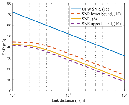
Fig. 4 plots the SNR versus the link distance between the transmitter and IRS $r_{q}$ for UPA-based XL-IRS, which has size $L_{y}=L_{z}=5\,$ m. The direction of the transmitter is $(\theta_{q},\phi_{q})=(\frac{\pi}{3},\frac{\pi}{6})$ and the location of the receiver is $(r_{p},\theta_{p},\phi_{p})=(200\,\mathrm{m},\frac{3\pi}{4},-\frac{\pi}{5})$ , respectively. The transmit SNR is $\bar{P}=100\,$ dB. It is observed that the bounds given in Theorem 1 are tight, and the conventional UPW model over-estimates the SNR values. In particular, for relatively small link distance $r_{q}$ , different SNR scalings versus $r_{q}$ are observed for the conventional UPW model and the newly considered non-UPW model, which leads to significantly different SNR values, e.g., by a difference about $25\,$ dB for $r_{q}=2\,$ m.

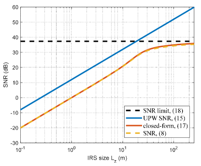
For ULA-based XL-IRS, Fig. 5 shows the SNR versus the IRS size $L_{z}$ based on the summation (LABEL:8), the derived closed-form expression (13), the asymptotic limit (4), and that under the conventional UPW model (12). The locations of the transmitter and receiver are $(r_{q},\theta_{q},\phi_{q})=(10\,\mathrm{m},\frac{\pi}{3},\frac{\pi}{6})$ and $(r_{p},\theta_{p},\phi_{p})=(100\,\mathrm{m},\frac{3\pi}{4},-\frac{\pi}{5})$ , respectively, and the transmit SNR is $\bar{P}=120\,$ dB. It is firstly observed that the closed-form expression (13) and the asymptotic limit (4) match well with the actual values. Furthermore, similar to Fig. 3, there exists significant gap between the conventional UPW model and our considered model. In particular, as $L_{z}$ becomes sufficiently large, while the SNR under the UPW model increases unboundedly, that under our considered model approaches to a constant value specified in (4). This again demonstrates the importance of proper channel modelling for communications aided by XL-IRS.

V Conclusions

This paper studied the mathematical modelling and performance analysis of wireless communication aided by XL-IRS. By taking into account the variations in signal’s amplitude and projected aperture across different reflecting elements, we firstly derived tight lower- and upper-bounds of the receiver SNR for the general UPA-based XL-IRS. To gain more insights, the special case of ULA-based XL-IRS was also considered, for which a closed-form SNR expression in terms of the ULA size and transmitter/receiver locations was derived. Numerical results verified our theoretical analysis and demonstrated the importance of proper channel modelling for wireless communications aided by XL-IRS.

Appendix A Proof of Lemma 1

The double integral in (11) reduces to the following form under the assumption of $\Phi_{q},\Phi_{p}\ll\frac{r_{q}}{L_{y}}$ and $\Omega_{q},\Omega_{p}\ll\frac{r_{q}}{L_{z}}$ .

	$\displaystyle I_{1}$	$\displaystyle\simeq\int_{0}^{2\pi}\mathrm{d}\zeta\int_{0}^{R}\frac{r\mathrm{d}r}{[(1+\frac{r^{2}}{r_{q}^{2}})(1+\frac{r^{2}}{r_{p}^{2}})]^{3/4}}$
		$\displaystyle=2\pi r_{q}^{2}\int_{0}^{\frac{R}{r_{q}}}\frac{r\mathrm{d}r}{[(r^{2}+1)(\rho^{2}r^{2}+1)]^{3/4}}.$		(15)

By letting $r=\tan\alpha$ , (A) can be simplified as

I_{1}=2\pi r_{q}^{2}\int_{0}^{\arctan\frac{R}{r_{q}}}\frac{\sin\alpha\mathrm{d}\alpha}{[\rho^{2}+(1-\rho^{2})\cos^{2}\alpha]^{3/4}}.

(16)

We first consider the case of $0<\rho<1$ . By letting $v=\frac{\sqrt{1-\rho^{2}}}{\rho}\cos\alpha$ , $I_{1}$ can be further expressed as

	$\displaystyle I_{1}$	$\displaystyle=2\pi r_{q}^{2}\frac{\rho^{-1/2}}{\sqrt{1-\rho^{2}}}\int_{\frac{\sqrt{1-\rho^{2}}}{\rho}\cos(\arctan\frac{R}{r_{q}})}^{\frac{\sqrt{1-\rho^{2}}}{\rho}}\frac{\mathrm{d}v}{(v^{2}+1)^{3/4}}.$
		$\displaystyle=4\pi r_{q}^{2}\frac{\rho^{-1/2}}{\sqrt{1-\rho^{2}}}\int_{\arctan(\frac{\sqrt{1-\rho^{2}}}{\rho}\cos(\arctan\frac{R}{r_{q}}))}^{\arctan\frac{\sqrt{1-\rho^{2}}}{\rho}}\frac{\mathrm{d}\frac{\varphi}{2}}{\sqrt{1-2\sin^{2}\frac{\varphi}{2}}},$		(17)

where the last equality follows by a change of variable as $v=\tan\varphi$ . According to the definition of incomplete Elliptic Integral of the First Kind, (A) can be written as

I_{1}=4\pi r_{q}^{2}\frac{\rho^{-1/2}}{\sqrt{1-\rho^{2}}}\sqrt{G(R)},

(18)

where $G(R)$ is defined in (10).

By substituting (18) into (11) and with Theorem 1, the first case of (9) in Lemma 1 can be obtained.

For the special case of $\rho=1$ , i.e., $r_{q}=r_{p}$ , (9) can be obtained from the integral in (9), where under the condition of Lemma 1, we have

	$\displaystyle I_{2}$	$\displaystyle=\int_{-\frac{L_{z}}{2}}^{\frac{L_{z}}{2}}\int_{-\frac{L_{y}}{2}}^{\frac{L_{y}}{2}}\frac{\mathrm{d}y\mathrm{d}z}{(1+\frac{y^{2}}{r_{q}^{2}}+\frac{z^{2}}{r_{q}^{2}})^{3/2}}$
		$\displaystyle=4r_{q}^{2}\arctan\frac{(\frac{L_{y}}{2r_{q}})(\frac{L_{z}}{2r_{q}})}{\sqrt{(\frac{L_{y}}{2r_{q}})^{2}+(\frac{L_{z}}{2r_{q}})^{2}+1}}.$		(19)

By substituting (A) into (9), the second case of (9) then follows.

Appendix B Proof of Lemma 3

By applying a change of variable as $t=\frac{z}{r_{q}}$ , the integral in (16) can be expressed as

I=\int_{-\frac{L_{z}}{2r_{q}}}^{\frac{L_{z}}{2r_{q}}}\frac{r_{q}\mathrm{d}t}{[(1-2t\cos\theta_{q}+t^{2})(1-2\rho t\cos\theta_{p}+\rho^{2}t^{2})]^{3/4}}.

(20)

By letting $u=\frac{t-\cos\theta_{q}}{\sin\theta_{q}}$ , $I$ can be further written as

I=\frac{r_{q}}{\sqrt{\sin\theta_{q}}}\int_{u_{1}}^{u_{2}}\frac{\mathrm{d}u}{(u^{2}+1)^{3/4}[(u^{2}+1)X+Yu+1+Z]^{3/4}},

(21)

where

	$\displaystyle u_{1}=-\frac{L_{z}/2+r_{q}\cos\theta_{q}}{r_{q}\sin\theta_{q}},u_{2}=\frac{L_{z}/2-r_{q}\cos\theta_{q}}{r_{q}\sin\theta_{q}},$
	$\displaystyle X=\rho^{2}\sin^{2}\theta_{q},$
	$\displaystyle Y=2\rho^{2}\sin\theta_{q}\cos\theta_{q}-2\rho\sin\theta_{q}\cos\theta_{p},$
	$\displaystyle Z=\rho^{2}\cos^{2}\theta_{q}-2\rho\cos\theta_{q}\cos\theta_{p}-\rho^{2}\sin^{2}\theta_{q}.$

Then by letting $u=\tan\varphi$ , (21) can be simplified as

I=\frac{r_{q}}{\sqrt{\sin\theta_{q}}}\int_{\varphi_{1}}^{\varphi_{2}}\frac{\cos\varphi\mathrm{d}\varphi}{[X+Y\sin\varphi\cos\varphi+(1+Z)\cos^{2}\varphi]^{3/4}},

(22)

where $\varphi_{1}=-\arctan\frac{L_{z}/2+r_{q}\cos\theta_{q}}{r_{q}\sin\theta_{q}}$ and $\varphi_{2}=\arctan\frac{L_{z}/2-r_{q}\cos\theta_{q}}{r_{q}\sin\theta_{q}}$ .

Under the condition of Lemma 3, we have $\rho\ll 1$ , and hence $X,Y,Z\ll 1$ . Thus, (22) reduces to

I\simeq\frac{r_{q}}{\sqrt{\sin\theta_{q}}}\int_{\varphi_{1}}^{\varphi_{2}}\frac{\mathrm{d}\varphi}{\sqrt{\cos\varphi}}.

(23)

Based on the definition of incomplete Elliptic Integral of the First Kind, we have

I=\frac{2r_{q}}{\sqrt{\sin\theta_{q}}}\bigg{[}F(-\frac{\varphi_{1}}{2}|2)+F(\frac{\varphi_{2}}{2}|2)\bigg{]}.

(24)

With the identities that $\alpha_{1}=-\varphi_{1}$ and $\alpha_{2}=\varphi_{2}$ , and by substituting (24) into (16), the proof of Lemma 3 is completed.

References

[1] Q. Wu, S. Zhang, B. Zheng, C. You, and R. Zhang, “Intelligent reflecting surface aided wireless communications: A tutorial,” IEEE Trans. Commun., vol. 69, no. 5, pp. 3313–3351, May 2021.
[2] Q. Wu and R. Zhang, “Intelligent reflecting surface enhanced wireless network via joint active and passive beamforming,” IEEE Trans. Wireless Commun., vol. 18, no. 11, pp. 5394–5409, Nov. 2019.
[3] C. Huang, A. Zappone, G. C. Alexandropoulos, M. Debbah, and C. Yuen, “Reconfigurable intelligent surfaces for energy efficiency in wireless communication,” IEEE Trans. Wireless Commun., vol. 18, no. 8, pp. 4157–4170, Aug. 2019.
[4] Q. Wu and R. Zhang, “Towards smart and reconfigurable environment: Intelligent reflecting surface aided wireless network,” IEEE Commun. Mag., vol. 58, no. 1, pp. 106–112, Jan. 2020.
[5] W. Tang et al., “Wireless communications with reconfigurable intelligent surface: Path loss modeling and experimental measurement,” IEEE Trans. Wireless Commun., vol. 20, no. 1, pp. 421–439, Jan. 2021.
[6] M. Di Renzo et al., “Smart radio environments empowered by reconfigurable intelligent surfaces: How it works, state of research, and the road ahead,” IEEE J. Sel. Areas Commun., vol. 38, no. 11, pp. 2450–2525, Nov. 2020.
[7] H. Lu, Y. Zeng, S. Jin, and R. Zhang, “Aerial intelligent reflecting surface: Joint placement and passive beamforming design with 3D beam flattening,” IEEE Trans. Wireless Commun., Early Access.
[8] Ö. Özdogan, E. Björnson, and E. G. Larsson, “Intelligent reflecting surfaces: Physics, propagation, and pathloss modeling,” IEEE Wireless Commun. Lett., vol. 9, no. 5, pp. 581–585, May 2019.
[9] E. Björnson and L. Sanguinetti, “Demystifying the power scaling law of intelligent reflecting surfaces and metasurfaces,” in Proc. IEEE Int. Workshop Comput. Adv. Multi Sensor Adapt. Process., Dec. 2019, pp. 549–553.
[10] H. Lu and Y. Zeng, “How does performance scale with antenna number for extremely large-scale MIMO?” in Proc. IEEE Int. Conf. (ICC), 2021.
[11] ——, “Communicating with extremely large-scale array/surface: Unified modelling and performance analysis,” 2021, arXiv:2104.13162. [Online]. Available: https://arxiv.org/abs/2104.13162.
[12] S. Hu, F. Rusek, and O. Edfors, “Beyond massive MIMO: The potential of data transmission with large intelligent surfaces,” IEEE Trans. Signal Process., vol. 66, no. 10, pp. 2746–2758, May 2018.
[13] D. Dardari, “Communicating with large intelligent surfaces: Fundamental limits and models,” IEEE J. Sel. Areas Commun., vol. 38, no. 11, pp. 2526–2537, Nov. 2020.
[14] E. Björnson and L. Sanguinetti, “Power scaling laws and near-field behaviors of massive MIMO and intelligent reflecting surfaces,” IEEE Open J. Commun. Society, vol. 1, pp. 1306–1324, 2020.
[15] Y. L. Luke, “Approximations for elliptic integrals,” Mathematics of Computation, vol. 22, no. 103, pp. 627–634, 1968.
[16] G. B. Thomas and R. L. Finney, Calculus. Addison-Wesley Publishing Company, 1961.