Within-group fairness: A guidance for more sound between-group fairness
Abstract
As they have a vital effect on social decision-making, AI algorithms not only should be accurate and but also should not pose unfairness against certain sensitive groups (e.g., non-white, women). Various specially designed AI algorithms to ensure trained AI models to be fair between sensitive groups have been developed. In this paper, we raise a new issue that between-group fair AI models could treat individuals in a same sensitive group unfairly. We introduce a new concept of fairness so-called within-group fairness which requires that AI models should be fair for those in a same sensitive group as well as those in different sensitive groups. We materialize the concept of within-group fairness by proposing corresponding mathematical definitions and developing learning algorithms to control within-group fairness and between-group fairness simultaneously. Numerical studies show that the proposed learning algorithms improve within-group fairness without sacrificing accuracy as well as between-group fairness.
1 Introduction
Recently, AI (Artificial Intelligence) is being used as decision-making tools in various domains such as credit scoring, criminal risk assessment, education of college admissions [1]. As AI has a wide range of influences on human social life, issues of transparency and ethics of AI are emerging. However, it is widely known that due to the existence of historical bias in data against ethics or regulatory frameworks for fairness, trained AI models based on such biased data could also impose bias or unfairness against a certain sensitive group (e.g., non-white, women) [2, 3]. Therefore, designing an AI algorithm which is accurate and fair simultaneously has become a crucial research topic.
Demographic disparities due to AI, which refer to socially unacceptable bias that an AI model favors certain groups (e.g., white, men) over other groups (e.g., black, women), have been observed frequently in many applications of AI such as COMPAS recidivism risk assessment [1], Amazon’s prime free same-day delivery [4], credit score evaluation [5] to name just a few. Many studies have been done recently to develop AI algorithms which remove or alleviate such demographic disparities in trained AI models so that they will treat sensitive groups as equally as possible. In general, these methods try to search AI models which are not only accurate but also similar between sensitive groups in a certain sense. For an example of similarity, it is required that accuracies of an AI model for each sensitive group are similar [6]. Hereinafter, criteria of fairness requiring similarity between sensitive groups are referred to as between-groups fairness (BGF).
In this paper, we consider a new concept of fairness so called within-group fairness (WGF) which arises as a new problem when we try to enforce BGF into AI algorithms. Generally speaking, within-group unfairness occurs when there is an individual who is positively treated compared to others in a same sensitive group by an AI model trained without BGF constraints but becomes negatively treated by an AI model trained with BGF constraints.
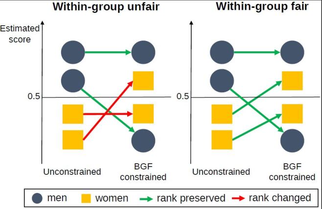
For an illustrative example of WGF, consider a college admission problem where gender (men vs women) is a sensitive variable. Let and be the input vector and the corresponding output label where represents the information of a candidate student such as GPA at high school, SAT score, etc. and is the admission result where 0 and 1 mean the rejection and acceptance of the college admission, respectively. The Bayes classifier accepts a student with when Suppose that there are two women ‘’ and ‘’ with the input vectors and respectively and the AI model trained without BGF constraints estimates Then, within-group unfairness occurs when an AI model trained with BGF constraints results in In this situation, which is illustrated in the left panel of Figure 1, ‘’ could claim that the AI model trained with BGF constraints mistreats her and so it is unfair. We will show in Section 5 that there exists non-negligible within-group unfairness in AI models trained on real data with BGF constraints.
Within-group unfairness arises because most existing learning algorithms for BGF force certain statistics (e.g. rate of positive prediction, misclassification error rate, etc.) of a trained AI model being similar across sensitive groups but do not care about what happens to individuals in a same sensitive group at all. For within-group fairness, a desirable AI model is expected at least to preserve the ranks between and regardless of estimating with or without BGF constraints, which is depicted in the right panel of Figure 1.
Our contributions are three folds. We first define the concept of WGF rigorously. Then we develop learning algorithms which compromise BGF and WGF as well as accuracy. Finally, we show empirically that the proposed learning algorithms improve WGF while maintaining accuracy and BGF.
Remark. One may argue that training data are prone to bias due to historical prejudices and discriminations, and hence a trained AI model is also biased and socially unacceptable. On the other hand, a trained AI model with BGF constraints does not have such bias and hence is socially acceptable. Therefore, it would be by no means reasonable to claim unfairness based on discrepancies between socially unacceptable and acceptable AI models. However, note that historical bias in training data is about bias between sensitive groups but not for individuals in a same sensitive group. For WGF, we implicitly assume that no historical bias among individuals in a same sensitive group exists in training data, which is not too absurd, and thus there is no reason for a trained AI model without BGF constraints to treat individuals in a same sensitive group unfairly. This assumption, of course, needs more debates which we leave as future work.
The paper is organized as follows. In Section 2, we briefly review methods for BGF, and in Sections 3 and 4, we propose mathematical definitions of WGF and develop corresponding learning algorithms for classifiers and score functions, respectively. The results of numerical studies are presented in Section 5, and remarks about reflecting WGF to pre- and post processing algorithms for BGF are given in Section 6. Concluding remarks follow in Section 7.
2 Review of between-group fairness
While it is completely new, the concept of WGF is a by-product of BGF and thus it is helpful to review learning methods for BGF. In this section, we review the definitions of BGF and related studies.
We let be a set of training data of size which are independent copies of a random vector defined on where We consider a binary classification problem, which means and for notational simplicity, we let , where refers to the unprivileged group and refers to the privileged group. Whenever the probability is mentioned, we mean it by either the probability of or its empirical counterpart unless there is any confusion.
In this paper, we consider AI algorithms which yield a real-valued function so called a score function which assigns positive labeled instances higher scores than negative labeled instances. An example of the score function is the conditional class probability In most human-related decision makings, real-valued score functions are popularly used (e.g. scores for credit scoring).
Let be a given set of score functions, in which we search an optimal score function in a certain sense (e.g. minimizing the cross-entropy for classification problems). Examples of are linear functions, reproducing kernel Hilbert space and deep neural networks to name a few. For a given the corresponding classifier is defined as
2.1 Definition of between-group fairness
For a given score function and a sensitive group , we consider the group performance function of given as
| (1) |
for events and that might depend on and The group performance function in (1), which is considered by [7], includes various performance functions used in fairness AI. We summarize representative group performance functions having the form of (1) in Table 1.
For given group performance functions we say that satisfies the BGF constraint with respect to if A relaxed version of the BGF constraint so called the -BGF constraint, is frequently considered, which requires for a given Typically, AI algorithms search an optimal function among those satisfying the -BGF constraint with respect to given group performance functions
2.2 Related works
Several learning algorithms have been proposed to find an accurate model satisfying a given BGF constraint, which are categorized into three groups. In this subsection, we review some methods for each group.
Pre-processing methods: Pre-processing methods remove bias in training data or find a fair representation with respect to sensitive variables before the training phase and learn AI models based on de-biased data or fair representation [11, 12, 13, 14, 15, 16, 17, 18, 19]. [11] suggested pre-processing methods to eliminate bias in training data by use of label changing, reweighing and sampling. Based on the idea that transformed data should not be able to predict the sensitive variable, [13] proposed a transformation of input variables for eliminating the disparate impact. To find a fair representation, [12, 14] proposed a data transformation mapping for preserving accuracy and alleviating discrimination simultaneously. Pre-processing methods for fair learning on text data were studied by [15, 16].
In-processing methods: In-processing methods generally train an AI model by minimizing a given cost function (e.g. the cross-entropy, the sum of squared residuals, the empirical AUC etc.) subject to a -BGF constraint. Most group performance functions are not differentiable, and thus various surrogated group performance functions and corresponding -BGF constraints have been proposed [20, 21, 22, 23, 6, 24, 25, 26, 7, 27, 28]. [20] used a fairness regularizer which is an approximation of the mutual information between the sensitive variable and the target variable. [23, 6] proposed covariance-type fairness constraints as tractable proxies targeting the disparate impact and the equality of the false positive or negative rate, and [24] used a linear surrogated group performance function for the equalized odds. On the other hand, [25, 7] derived an optimal classifier for a constrained fair classification as a form of an instance-dependent threshold. Also, for fair score functions, [27] proposed fairness constraints based on ROC curves of each sensitive group.
Post-processing methods: Post-processing methods first learn an AI model without any BGF constraint and then transform the decision boundary or score function of the trained AI model for each sensitive group to satisfy given BGF criteria [29, 30, 9, 31, 32, 33, 34, 35]. [9, 33] suggested finding sensitive group dependent thresholds to get a fair classifier with respect to equal opportunity. [34, 35] developed an algorithm to transform the original score function to achieve a BGF constraint.
3 Within-group fairness for classifiers
We assume that there exists a known optimal classifier which could be the Bayes classifier or its estimate. For example, we can use for where is the unconstrained minimizer of the cross-entropy on We mostly focus on in-processing methods for the BGF and explain how to reflect WGF into a learning procedure. Remarks about how to reflect WGF to pre- and post-processing methods are given in Section 6.
3.1 Definition of within-group fairness
Conceptually, WGF means that the classifier and have the same ranks in each sensitive group. That is, for two individuals and in a same sensitive group with WGF requires that To materialize this concept of WGF, we define the WGF constraint as
| (2) |
for each Similar to the BGF, we relax the constraint (2) by requiring that either of the two probabilities is small. That is, we say that satisfies the -WGF constraint for a given if
| (3) |
where
3.2 Directional within-group fairness
Many BGF constraints have their own implicit directions toward which the classifier is expected to be guided in the training phase. We can design a special WGF constraint reflecting the implicit direction of a given BGF constraint which results in more desirable classifiers (better guided, more fair and frequently more accurate). Below, we present two such WGF constraints.
Disparate impact: Note that the disparate impact requires that
Suppose that Then, we expect that a desirable classifier achieves this BGF constraint by increasing from and decreasing from To reflect this direction, we can enforce a learning algorithm to search a classifier satisfying and Based on this argument, we define the directional -WGF constraint for the disparate impact as
| (4) |
Equal opportunity: The equal opportunity constraint is given as
Suppose that A similar argument for the disparate impact leads us to define the directional -WGF constraint for the equal opportunity as
| (5) |
and
| (6) |
where
3.3 Learning with doubly-group fairness constraints
We say that satisfies the -doubly-group fairness constraint if and where is a given BGF constraint and is the corresponding WGF constraint proposed in the previous two subsections. In this section, we propose a relaxed version of for easy computation. As we review in Section 2, many relaxed versions of have been proposed already.
The WGF constraints considered in Sections 3.1 and 3.2 are hard to be used as themselves in the training phase since they are neither convex nor continuous. A standard approach to resolve this problem is to use a convex surrogated function. For example, a surrogated version of the WGF constraint (3) is where
| (7) |
where and is a convex surrogated function of the indicator function In this paper, we use the hinge function given as as a convex surrogated function which is popularly used for fair AI [21, 24, 36]. The surrogated versions for the other WGF constraints are derived similarly. Finally, we estimate by that minimizes the regularized cost function
| (8) |
where is a given cost function (e.g. the cross-entropy) and and are the surrogated constraints of and respectively. The nonnegative constants and are regularization parameters which are selected so that satisfies and
3.4 Related notions with within-group fairness
There are several fairness concepts which are somehow related to WGF. However, the existing concepts are quite different from our WGF.
-
1.
Unified fairness: [37] used the term ‘within-group fairness’. However, WGF of [37] is different from our WGF. [37] measured individual-level benefits of a given prediction model and they defined the model to be WGF if the individual benefits in each group are similar. They also illustrated that WGF keeps decreasing as BGF increases. Our WGF is nothing to do with individual-level benefits. Our WGF can be high even when individual-level benefits are not similar. Also, our WGF can increase even when BGF increases.
-
2.
Slack consistency: [38] proposed the ‘slack consistency’ which requires that the estimated scores of each individual should be monotonic with respect to slack variables used in fairness constraints. Slack consistency does not guarantee within-group fairness because the ranks of the estimated scores can change even when they move monotonically.
4 Within-group fairness for score functions
Similarly to classifiers, the WGF for score functions requires that when and vice versa for two individuals and in a same sensitive group, where is a known optimal score function such as the conditional class probability or its estimate. To realize this concept, we define the WGF constraint for a score function as for where is the Kendall’s between and conditional on that is
where and are independent copies of In turn, the -WGF constraint for a score function is
Similarly for classifiers, we need a convex surrogated version of the -WGF constraint and a candidate would be where
and is a convex surrogated function of such as the
5 Numerical studies
We investigate the impacts of the WGF constraints on the prediction accuracy as well as the BGF by analyzing real-world datasets. We consider linear logistic and deep neural network (DNN) models for and use the cross-entropy for For DNN, fully connected neural networks with one hidden layer and many hidden nodes are used. We train the models by the gradient descent algorithm [39] implemented by Python with related libraries pytorch, scikit-learn, numpy. The SGD optimizer is used with momentum 0.9 and a learning rate of either 0.1 or 0.01 depending on the dataset. We use the unconstrained minimizer of for
Datasets. We analyze four real world datasets, which are popularly used in fairness AI research and publicly available: (i) The Adult Income dataset (Adult, [5]); (ii) The Bank Marketing dataset(Bank, [5]); (iii) The Law School dataset (LSAC, [40]); (iv) The Compas Propublica Risk Assessment dataset (COMPAS, [41]). Except for the dataset Adult, we split the training and test datasets randomly by 8:2 ratio and repeat 5 times training/test splits for performance evaluation.
5.1 Within-group fair classifiers
We consider following group performance functions for the BGF: the disparate impact (DI) [8] and the disparate mistreatment w.r.t. error rate [6], which are defined as
Note that the DI is directional while the ME is not. For the surrogated BGF constraints, we replace the indicator function with the hinge function in calculating the BGF constraints as is done by [21, 36]. We name the corresponding BGF constraints by Hinge-DI and Hinge-ME respectively. The results for other surrogated constraints such as the covariance type constraints proposed by [23, 6] and the linear surrogated functions considered in [42] are presented in the Supplementary material. In addition, the results for the equal opportunity constraint are summarized in the Supplementary material.
For investigating the impacts of WGF on trained classifiers, we first fix the for each BGF constraint, and we choose the regularization parameters and to make the classifier minimizing the regularized cost function (8) satisfy the -BGF constraint. Then, we assess the prediction accuracy and the degree of WGF of
5.1.1 Targeting for disparate impact
Table 2 presents the three tables comparing the results of the unconstrained DNN classifier () and three DNN classifiers () trained on the dataset Adult: (i) only with the DI constraint, (ii) with the DI and WGF constraints and (iii) with the DI and directional WGF (dWGF) constraints. We let be around 0.03. The numbers marked in red are subjects treated unfairly with respect to the dWGF. Note that the numbers of unfairly treated subjects are reduced much with the WGF and dWGF constraints and the dWGF constraint is more effective. We report that the accuracies of the three classifiers on the test data are 0.837, 0.840 and 0.839, respectively, which indicates that the WGF and dWGF constraints improve the WGF without hampering the accuracy. Compared to the dWGF, the WGF constraint is less effective, which is observed consistently for different datasets when a BGF constraint is directional. See Table 2 in the Supplementary material for the corresponding numerical results. Thus, hereafter we consider the dWGF only for the DI which has an implicit direction.
| Only with the DI constraint | |||||
|---|---|---|---|---|---|
| 4,592 | 350 | 7,966 | 86 | ||
| 13 | 466 | 945 | 1,863 | ||
| With the DI and WGF constraints | |||||
| 4,703 | 239 | 8,021 | 31 | ||
| 27 | 452 | 1,156 | 1,652 | ||
| With the DI and dWGF constraints | |||||
| 4,718 | 224 | 8,024 | 28 | ||
| 18 | 461 | 1,178 | 1,630 | ||
Table 3 summarizes the performances of the three classifiers - and the two classifiers trained with the DI constraint and the DI and dWGF constraints (doubly-fair, DF), respectively. In Table 3, we report the accuracies as well as the values of DI and dWGF terms (i.e., and respectively). We observe that the DF classifier improves the dWGF while keeping that the DI values and accuracies are favorably comparable to those of the BGF classifier. For reference, the performances with the WGF constraint are summarized in the Supplementary material.
| Linear model | DNN model | |||||||
|---|---|---|---|---|---|---|---|---|
| Dataset | Method | ACC | DI | dWGF | ACC | DI | dWGF | |
| Adult | Uncons. | 0.852 | 0.172 | 0.000 | 0.853 | 0.170 | 0.000 | |
| Hinge-DI | 0.833 | 0.028 | 0.005 | 0.837 | 0.029 | 0.008 | ||
| Hinge-DI-DF | 0.836 | 0.028 | 0.003 | 0.839 | 0.026 | 0.003 | ||
| Bank | Uncons. | 0.908 | 0.195 | 0.000 | 0.904 | 0.236 | 0.000 | |
| Hinge-DI | 0.901 | 0.024 | 0.018 | 0.899 | 0.029 | 0.033 | ||
| Hinge-DI-DF | 0.904 | 0.021 | 0.007 | 0.905 | 0.029 | 0.032 | ||
| LSAC | Uncons. | 0.823 | 0.120 | 0.000 | 0.856 | 0.131 | 0.000 | |
| Hinge-DI | 0.809 | 0.016 | 0.014 | 0.816 | 0.032 | 0.064 | ||
| Hinge-DI-DF | 0.813 | 0.018 | 0.009 | 0.809 | 0.029 | 0.047 | ||
| COMPAS | Uncons. | 0.757 | 0.164 | 0.000 | 0.757 | 0.162 | 0.000 | |
| Hinge-DI | 0.641 | 0.024 | 0.153 | 0.639 | 0.030 | 0.142 | ||
| Hinge-DI-DF | 0.618 | 0.025 | 0.145 | 0.654 | 0.033 | 0.120 | ||
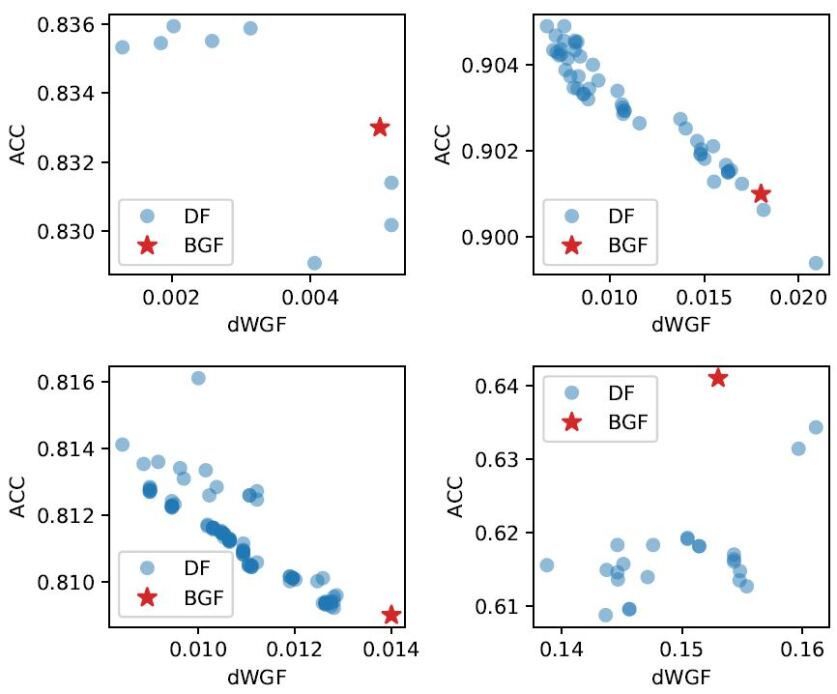
To investigate the sensitivity of the accuracy to the degree of WGF, the scatter plots between various dWGF values and the corresponding accuracies for the DF linear logistic model are given in Figure 2, where the DI value is fixed around 0.03. The accuracies are not sensitive to the dWGF values. Moreover, for the datasets Adult, Bank and LSAC, the accuracies keep increasing as the dWGF value decreases.
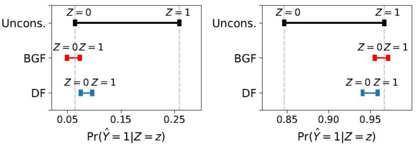
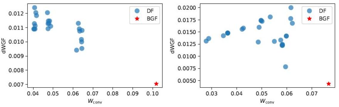
While we analyzed the datasets Bank and LSAC, we found an undesirable aspect of the learning algorithm only with the DI constraint. The corresponding classifiers improve the DI by decreasing (or increasing) the probabilities and simultaneously compared to and A better way to improve the DI would be to increase and decrease when Figures 3 show that this undesirable aspect disappears when the dWGF constraint is considered.
5.1.2 Targeting for disparate mistreatment
The results of the performances of the DF classifier with the ME as a BGF constraint are presented in Table 4. Since the ME has no implicit direction, we use the undirectional WGF constraint. The overall conclusions are similar to those for the DI and dWGF constraints. That is, the undirectional WGF constraint also works well.
| Linear model | DNN model | |||||||
|---|---|---|---|---|---|---|---|---|
| Dataset | Method | ACC | ME | WGF | ACC | ME | WGF | |
| Adult | Uncons. | 0.852 | 0.117 | 0.000 | 0.853 | 0.105 | 0.000 | |
| Hinge-ME | 0.834 | 0.060 | 0.005 | 0.822 | 0.025 | 0.059 | ||
| Hinge-ME-DF | 0.834 | 0.060 | 0.005 | 0.825 | 0.031 | 0.026 | ||
| Bank | Uncons. | 0.908 | 0.177 | 0.000 | 0.904 | 0.174 | 0.000 | |
| Hinge-ME | 0.740 | 0.044 | 0.068 | 0.902 | 0.164 | 0.076 | ||
| Hinge-ME-DF | 0.749 | 0.045 | 0.020 | 0.897 | 0.165 | 0.047 | ||
| LSAC | Uncons. | 0.823 | 0.090 | 0.000 | 0.856 | 0.071 | 0.000 | |
| Hinge-ME | 0.759 | 0.028 | 0.038 | 0.815 | 0.044 | 0.040 | ||
| Hinge-ME-DF | 0.742 | 0.020 | 0.017 | 0.803 | 0.038 | 0.001 | ||
| COMPAS | Uncons. | 0.757 | 0.022 | 0.000 | 0.757 | 0.024 | 0.000 | |
| Hinge-ME | 0.740 | 0.020 | 0.018 | 0.738 | 0.016 | 0.018 | ||
| Hinge-ME-DF | 0.743 | 0.018 | 0.001 | 0.757 | 0.017 | 0.001 | ||
5.2 Within-group fair for score function
In this section, we examine the WGF constraint for score functions. We choose the logistic loss (binary cross-entropy, BCE) and AUC (area under the ROC) as evaluation metrics for prediction accuracy. For the BGF, we consider the mean score parity (MSP, [10]):
where is the sigmoid function. To check how much the estimated score function is within-group fair, we calculate the Kendall’s between and the ground-truth score function on the test data for each sensitive group, and then we average them, which is denoted by in Table 5. We choose the regularization parameters and such that of is as close to 1 as possible while maintaining the MSP value around 0.03.
Table 5 amply shows that the DF score function always improves the degree of WGF (measured by ) and the accuracy in terms of AUC simultaneously while keeping the degree of BGF at a reasonable level. With respect to the BCE, the BGF and DF score functions are similar. The superiority of the DF score function in terms of AUC compared with the BGF score function is partly because the WGF constraint shrinks the estimated score toward the ground-truth score (Uncons. in Table 5) which is expected to be most accurate. Based on these results, we conclude that the WGF constraint is a useful guide to find a better score function with respect to AUC as well as the WGF.
| Linear model | DNN model | |||||||||
|---|---|---|---|---|---|---|---|---|---|---|
| Dataset | Method | BCE | AUC | MSP | BCE | AUC | MSP | |||
| Adult | Uncons. | 0.319 | 0.905 | 0.173 | 1.000 | 0.315 | 0.908 | 0.178 | 1.000 | |
| BGF | 0.358 | 0.879 | 0.037 | 0.854 | 0.353 | 0.879 | 0.035 | 0.805 | ||
| DF | 0.368 | 0.882 | 0.033 | 0.908 | 0.364 | 0.885 | 0.035 | 0.891 | ||
| Bank | Uncons. | 0.214 | 0.932 | 0.217 | 1.000 | 0.237 | 0.926 | 0.237 | 1.000 | |
| BGF | 0.235 | 0.906 | 0.036 | 0.706 | 0.270 | 0.908 | 0.033 | 0.671 | ||
| DF | 0.240 | 0.912 | 0.039 | 0.728 | 0.266 | 0.917 | 0.031 | 0.761 | ||
| LSAC | Uncons. | 0.434 | 0.732 | 0.125 | 1.000 | 0.359 | 0.831 | 0.142 | 1.000 | |
| BGF | 0.450 | 0.705 | 0.033 | 0.692 | 0.381 | 0.803 | 0.025 | 0.640 | ||
| DF | 0.557 | 0.717 | 0.031 | 0.719 | 0.383 | 0.809 | 0.028 | 0.738 | ||
| COMPAS | Uncons. | 0.511 | 0.822 | 0.122 | 1.000 | 0.506 | 0.824 | 0.118 | 1.000 | |
| BGF | 0.599 | 0.759 | 0.035 | 0.564 | 0.588 | 0.753 | 0.030 | 0.561 | ||
| DF | 0.597 | 0.792 | 0.038 | 0.720 | 0.597 | 0.766 | 0.028 | 0.623 | ||
6 Remarks on within-group fairness for pre- and post-processing methods
Various pre- and post-processing methods for fair AI have been proposed. An advantage of these methods compared to constrained methods is that the methods are simple, computationally efficient but yet reasonably accurate. In this section, we briefly explain how to reflect the WGF to pre- and post-processing methods for the BGF.
6.1 Pre-processing methods and within-group fairness
Basically, pre-processing methods transform the training data in a certain way to be between-group fair and train an AI model on the transformed data. To reflect the WGF, it suffices to add a WGF constraint in the training phase. Let be the transformed training data to be between-group fair and let be the corresponding cost function. Then, we learn a model by minimizing for
Table 6 presents the results of the models trained on the pre-processing training data and a WGF constraint for various values of where the DI is used as the BGF and thus the corresponding dWGF constraint is used. In this experiment, we use the linear logistic model and the Massaging [11] for the pre-processing. Surprisingly we observed that introducing the dWGF constraint to the pre-processing method helps to improve the BGF and WGF simultaneously without sacrificing the accuracies much.
| Method | Acc | DI | dWGF | |
|---|---|---|---|---|
| Massaging | - | 0.837 | 0.069 | 0.009 |
| Massaging + dWGF | 0.5 | 0.837 | 0.048 | 0.004 |
| 1.0 | 0.836 | 0.037 | 0.003 |
6.2 Post-processing methods and within-group fairness
For the BGF score functions, [35] developed an algorithm to obtain two monotonically nondecreasing transformations such that and are BGF in the sense that the distributions of and are the same. It is easy to check that the transformed score function is a perfectly WGF score function even though it depends on the sensitivity group variable Note that the algorithm in Section 4 yields score functions not depending on
7 Conclusion
In this paper, we introduced a new concept so called within-group fairness, which should be considered along with BGF when fair AI is a concern. Also, we proposed a regularization procedure to control the degree of WGF of the estimated classifiers and score functions. By analyzing four real-world datasets, we illustrated that the WGF constraints improve the degree of WGF without hampering BGF as well as accuracy. Moreover, in many cases, the WGF constraints are helpful to find more accurate prediction models.
A problem in the proposed learning algorithm for WGF is that using a surrogated constraint for a given WGF constraint is sometimes problematic. The learning algorithm can find a DF model which has a lower surrogated WGF value than that of a BGF model, but the original WGF value is much higher. See Section A.2 of Appendix for empirical evidence. A better surrogated WGF constraint to ensure a lower original WGF value would be useful.
Acknowledgments
This work was supported by Institute for Information & communications Technology Planning & Evaluation(IITP) grant funded by the Korea government(MSIT) (No. 2019-0-01396, Development of framework for analyzing, detecting, mitigating of bias in AI model and training data).
References
- [1] Julia Angwin, Jeff Larson, Surya Mattu, and Lauren Kirchner. Machine bias. ProPublica, May, 23:2016, 2016.
- [2] Jon Kleinberg, Jens Ludwig, Sendhil Mullainathan, and Ashesh Rambachan. Algorithmic fairness. In Aea papers and proceedings, volume 108, pages 22–27, 2018.
- [3] Ninareh Mehrabi, Fred Morstatter, Nripsuta Saxena, Kristina Lerman, and Aram Galstyan. A survey on bias and fairness in machine learning. arXiv preprint arXiv:1908.09635, 2019.
- [4] David Ingold and Spencer Soper. Amazon doesn’t consider the race of its customers. should it. Bloomberg, April, 1, 2016.
- [5] Dheeru Dua and Casey Graff. UCI machine learning repository, 2017.
- [6] Muhammad Bilal Zafar, Isabel Valera, Manuel Gomez-Rodriguez, and Krishna P Gummadi. Fairness Constraints: A Flexible Approach for Fair Classification. J. Mach. Learn. Res., 20(75):1–42, 2019.
- [7] L Elisa Celis, Lingxiao Huang, Vijay Keswani, and Nisheeth K Vishnoi. Classification with fairness constraints: A meta-algorithm with provable guarantees. In Proceedings of the Conference on Fairness, Accountability, and Transparency, pages 319–328, 2019.
- [8] Solon Barocas and Andrew D Selbst. Big data’s disparate impact. Calif. L. Rev., 104:671, 2016.
- [9] Moritz Hardt, Eric Price, and Nati Srebro. Equality of opportunity in supervised learning. In Advances in neural information processing systems, pages 3315–3323, 2016.
- [10] Amanda Coston, Karthikeyan Natesan Ramamurthy, Dennis Wei, Kush R Varshney, Skyler Speakman, Zairah Mustahsan, and Supriyo Chakraborty. Fair transfer learning with missing protected attributes. In Proceedings of the 2019 AAAI/ACM Conference on AI, Ethics, and Society, pages 91–98, 2019.
- [11] Faisal Kamiran and Toon Calders. Data preprocessing techniques for classification without discrimination. Knowledge and Information Systems, 33(1):1–33, 2012.
- [12] Rich Zemel, Yu Wu, Kevin Swersky, Toni Pitassi, and Cynthia Dwork. Learning fair representations. In International Conference on Machine Learning, pages 325–333, 2013.
- [13] Michael Feldman, Sorelle A Friedler, John Moeller, Carlos Scheidegger, and Suresh Venkatasubramanian. Certifying and removing disparate impact. In proceedings of the 21th ACM SIGKDD international conference on knowledge discovery and data mining, pages 259–268, 2015.
- [14] Flavio Calmon, Dennis Wei, Bhanukiran Vinzamuri, Karthikeyan Natesan Ramamurthy, and Kush R Varshney. Optimized pre-processing for discrimination prevention. In Advances in Neural Information Processing Systems, pages 3992–4001, 2017.
- [15] Lucas Dixon, John Li, Jeffrey Sorensen, Nithum Thain, and Lucy Vasserman. Measuring and mitigating unintended bias in text classification. In Proceedings of the 2018 AAAI/ACM Conference on AI, Ethics, and Society, pages 67–73, 2018.
- [16] Kellie Webster, Marta Recasens, Vera Axelrod, and Jason Baldridge. Mind the gap: A balanced corpus of gendered ambiguous pronouns. Transactions of the Association for Computational Linguistics, 6:605–617, 2018.
- [17] Depeng Xu, Shuhan Yuan, Lu Zhang, and Xintao Wu. Fairgan: Fairness-aware generative adversarial networks. In 2018 IEEE International Conference on Big Data (Big Data), pages 570–575. IEEE, 2018.
- [18] Elliot Creager, David Madras, Jörn-Henrik Jacobsen, Marissa Weis, Kevin Swersky, Toniann Pitassi, and Richard Zemel. Flexibly fair representation learning by disentanglement. In International Conference on Machine Learning, pages 1436–1445. PMLR, 2019.
- [19] Novi Quadrianto, Viktoriia Sharmanska, and Oliver Thomas. Discovering fair representations in the data domain. In Proceedings of the IEEE/CVF Conference on Computer Vision and Pattern Recognition, pages 8227–8236, 2019.
- [20] Toshihiro Kamishima, Shotaro Akaho, Hideki Asoh, and Jun Sakuma. Fairness-aware classifier with prejudice remover regularizer. In Joint European Conference on Machine Learning and Knowledge Discovery in Databases, pages 35–50. Springer, 2012.
- [21] Gabriel Goh, Andrew Cotter, Maya Gupta, and Michael P Friedlander. Satisfying real-world goals with dataset constraints. In Advances in Neural Information Processing Systems, pages 2415–2423, 2016.
- [22] Yahav Bechavod and Katrina Ligett. Learning fair classifiers: A regularization-inspired approach. arXiv preprint arXiv:1707.00044, pages 1733–1782, 2017.
- [23] Muhammad Bilal Zafar, Isabel Valera, Manuel Gomez Rogriguez, and Krishna P Gummadi. Fairness constraints: Mechanisms for fair classification. In Artificial Intelligence and Statistics, pages 962–970, 2017.
- [24] Michele Donini, Luca Oneto, Shai Ben-David, John S Shawe-Taylor, and Massimiliano Pontil. Empirical risk minimization under fairness constraints. In Advances in Neural Information Processing Systems, pages 2791–2801, 2018.
- [25] Aditya Krishna Menon and Robert C Williamson. The cost of fairness in binary classification. In Conference on Fairness, Accountability and Transparency, pages 107–118, 2018.
- [26] Harikrishna Narasimhan. Learning with complex loss functions and constraints. In International Conference on Artificial Intelligence and Statistics, pages 1646–1654. PMLR, 2018.
- [27] Robin Vogel, Aurélien Bellet, and Stéphan Clémençon. Learning Fair Scoring Functions: Fairness Definitions, Algorithms and Generalization Bounds for Bipartite Ranking. arXiv preprint arXiv:2002.08159, 2020.
- [28] Jaewoong Cho, Changho Suh, and Gyeongjo Hwang. A fair classifier using kernel density estimation. In 34th Conference on Neural Information Processing Systems, NeurIPS 2020. Conference on Neural Information Processing Systems, 2020.
- [29] Faisal Kamiran, Asim Karim, and Xiangliang Zhang. Decision theory for discrimination-aware classification. In 2012 IEEE 12th International Conference on Data Mining, pages 924–929. IEEE, 2012.
- [30] Benjamin Fish, Jeremy Kun, and Ádám D Lelkes. A confidence-based approach for balancing fairness and accuracy. In Proceedings of the 2016 SIAM International Conference on Data Mining, pages 144–152. SIAM, 2016.
- [31] Sam Corbett-Davies, Emma Pierson, Avi Feller, Sharad Goel, and Aziz Huq. Algorithmic decision making and the cost of fairness. In Proceedings of the 23rd acm sigkdd international conference on knowledge discovery and data mining, pages 797–806, 2017.
- [32] Geoff Pleiss, Manish Raghavan, Felix Wu, Jon Kleinberg, and Kilian Q Weinberger. On fairness and calibration. In Advances in Neural Information Processing Systems, pages 5680–5689, 2017.
- [33] Evgenii Chzhen, Christophe Denis, Mohamed Hebiri, Luca Oneto, and Massimiliano Pontil. Leveraging labeled and unlabeled data for consistent fair binary classification. In Advances in Neural Information Processing Systems, pages 12760–12770, 2019.
- [34] Dennis Wei, Karthikeyan Natesan Ramamurthy, and Flavio Calmon. Optimized Score Transformation for Fair Classification. volume 108 of Proceedings of Machine Learning Research, pages 1673–1683, Online, 26–28 Aug 2020. PMLR.
- [35] Ray Jiang, Aldo Pacchiano, Tom Stepleton, Heinrich Jiang, and Silvia Chiappa. Wasserstein fair classification. In Uncertainty in Artificial Intelligence, pages 862–872. PMLR, 2020.
- [36] Yongkai Wu, Lu Zhang, and Xintao Wu. Fairness-aware Classification: Criterion, Convexity, and Bounds. arXiv preprint arXiv:1809.04737, 2018.
- [37] Till Speicher, Hoda Heidari, Nina Grgic-Hlaca, Krishna P Gummadi, Adish Singla, Adrian Weller, and Muhammad Bilal Zafar. A unified approach to quantifying algorithmic unfairness: Measuring individual &group unfairness via inequality indices. In Proceedings of the 24th ACM SIGKDD International Conference on Knowledge Discovery & Data Mining, pages 2239–2248, 2018.
- [38] Ofir Nachum and Heinrich Jiang. Group-based fair learning leads to counter-intuitive predictions. arXiv preprint arXiv:1910.02097, 2019.
- [39] Léon Bottou. Large-scale machine learning with stochastic gradient descent. In Proceedings of COMPSTAT’2010, pages 177–186. Springer, 2010.
- [40] Linda F Wightman and Henry Ramsey. LSAC national longitudinal bar passage study. Law School Admission Council, 1998.
- [41] Jeff Larson, Surya Mattu, Lauren Kirchner, and Julia Angwin. How we analyzed the COMPAS recidivism algorithm. ProPublica (5 2016), 9(1), 2016.
- [42] Manisha Padala and Sujit Gujar. FNNC: Achieving Fairness through Neural Networks. pages 2249–2255, 07 2020.
- [43] Preethi Lahoti, Alex Beutel, Jilin Chen, Kang Lee, Flavien Prost, Nithum Thain, Xuezhi Wang, and Ed H Chi. Fairness without demographics through adversarially reweighted learning. arXiv preprint arXiv:2006.13114, 2020.
Appendix A Supplenmetary Material
A.1 Additional numerical studies for WGF classification
A.1.1 Targeting for disparate impact
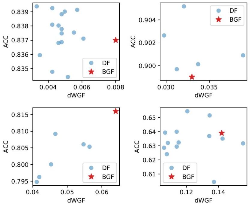
First, we investigate the sensitivity of the prediction accuracy to the degree of dWGF in the DNN model. Figure 4 shows the scatter plots between various dWGF values and the corresponding accuracies for the DF DNN model, where the DI is fixed around 0.03. The accuracies are not very sensitive to the dWGF values like the DF linear logistic model. Furthermore, for the datasets Adult, Bank and COMPAS, the DF classifiers have higher accuracies and lower dWGF values than the BGF classifier.
We also investigate how the dWGF constraint performs with surrogated BGF constraints other than Hinge-DI: (i) the covariance type constraint [23, 6], named by COV-DI; and (ii) the linear surrogated function, named by FNNC-DI [42]. Table 7 presents the results with various surrogated DI constraints and the dWGF constraint. In most cases, COV-DI and FNNC-DI give the results similar to Hinge-DI with or without the dWGF constraint and we consistently observe that considering the dWGF constraint together with the DI constraint helps to alleviate within-group fairness while maintaining similar levels of the accuracy and the DI. Note that for the dataset Adult, the DNN model with COV-DI constraint does not achieve the pre-specified DI value 0.03 regardless of the choice of tuning parameter. In contrast, the DNN model trained with the DI and dWGF constraints achieves the DI value 0.03 with a smaller value of dWGF. This observation is interesting since it implies that the dWGF constraint is helpful to increase even the BGF.
| Linear model | DNN model | |||||||
|---|---|---|---|---|---|---|---|---|
| Dataset | Method | ACC | DI | dWGF | ACC | DI | dWGF | |
| Adult | Uncons. | 0.852 | 0.172 | 0.000 | 0.853 | 0.170 | 0.000 | |
| COV-DI | 0.837 | 0.035 | 0.003 | 0.845 | 0.082 | 0.013 | ||
| COV-DI-DF | 0.837 | 0.030 | 0.001 | 0.840 | 0.025 | 0.007 | ||
| FNNC-DI | 0.834 | 0.023 | 0.003 | 0.838 | 0.023 | 0.006 | ||
| FNNC-DI-DF | 0.836 | 0.025 | 0.001 | 0.841 | 0.025 | 0.004 | ||
| Bank | Uncons. | 0.908 | 0.195 | 0.000 | 0.904 | 0.236 | 0.000 | |
| COV-DI | 0.904 | 0.019 | 0.009 | 0.906 | 0.019 | 0.036 | ||
| COV-DI-DF | 0.904 | 0.020 | 0.007 | 0.906 | 0.020 | 0.033 | ||
| FNNC-DI | 0.903 | 0.020 | 0.013 | 0.901 | 0.020 | 0.029 | ||
| FNNC-DI-DF | 0.905 | 0.020 | 0.008 | 0.900 | 0.010 | 0.027 | ||
| LSAC | Uncons. | 0.823 | 0.120 | 0.000 | 0.856 | 0.131 | 0.000 | |
| COV-DI | 0.808 | 0.015 | 0.014 | 0.859 | 0.052 | 0.020 | ||
| COV-DI-DF | 0.811 | 0.019 | 0.010 | 0.860 | 0.054 | 0.014 | ||
| FNNC-DI | 0.809 | 0.020 | 0.014 | 0.851 | 0.025 | 0.023 | ||
| FNNC-DI-DF | 0.809 | 0.014 | 0.010 | 0.844 | 0.010 | 0.019 | ||
| COMPAS | Uncons. | 0.757 | 0.164 | 0.000 | 0.757 | 0.162 | 0.000 | |
| COV-DI | 0.640 | 0.029 | 0.149 | 0.661 | 0.038 | 0.124 | ||
| COV-DI-DF | 0.620 | 0.024 | 0.135 | 0.650 | 0.028 | 0.097 | ||
| FNNC-DI | 0.646 | 0.037 | 0.146 | 0.646 | 0.032 | 0.133 | ||
| FNNC-DI-DF | 0.624 | 0.034 | 0.143 | 0.645 | 0.021 | 0.117 | ||
Next, we compare the dWGF and WGF constraints when targeting the DI with the hinge surrogated function in Table 8. In most cases, both the dWGF and WGF constraints are helpful to improve the WGF, while maintaining a similar level of accuracy and DI. It is noticeable that the DF classifier with the dWGF constraint is more accurate than that with the WGF constraint, which would be mainly because the DI constraint is directional.
| with the dWGF constraint | with the WGF constraint | |||||||
|---|---|---|---|---|---|---|---|---|
| Dataset | Method | ACC | DI | dWGF | ACC | DI | WGF | |
| Adult | Hinge-DI | 0.833 | 0.028 | 0.005 | 0.833 | 0.028 | 0.005 | |
| Hinge-DI-DF | 0.836 | 0.028 | 0.003 | 0.830 | 0.012 | 0.005 | ||
| Bank | Hinge-DI | 0.901 | 0.024 | 0.018 | 0.901 | 0.024 | 0.003 | |
| Hinge-DI-DF | 0.904 | 0.021 | 0.007 | 0.898 | 0.017 | 0.000 | ||
| LSAC | Hinge-DI | 0.809 | 0.017 | 0.014 | 0.809 | 0.017 | 0.014 | |
| Hinge-DI-DF | 0.813 | 0.018 | 0.009 | 0.810 | 0.016 | 0.011 | ||
| COMPAS | Hinge-DI | 0.641 | 0.024 | 0.153 | 0.641 | 0.024 | 0.136 | |
| Hinge-DI-DF | 0.618 | 0.025 | 0.145 | 0.594 | 0.018 | 0.088 | ||
A.1.2 Targeting for equal opportunity
We exam how the dWGF constraint works with the equal opportunity constraint given as
and the results are summarized in Table 9. For some cases, the dWGF constraint does not work at all (i.e., the dWGF values of the BGF and DF classifiers are the sames). This is partly because the surrogated dWGF constraint does not represent the original dWGF well, which is discussed in the following section.
| Linear model | DNN model | |||||||
|---|---|---|---|---|---|---|---|---|
| Dataset | Method | ACC | EOp | dWGF | ACC | EOp | dWGF | |
| Adult | Uncons. | 0.852 | 0.070 | 0.000 | 0.853 | 0.076 | 0.000 | |
| Hinge-EOp | 0.851 | 0.011 | 0.002 | 0.854 | 0.012 | 0.030 | ||
| Hinge-EOp-DF | 0.853 | 0.016 | 0.001 | 0.854 | 0.015 | 0.012 | ||
| FNNC-EOp | 0.851 | 0.013 | 0.012 | 0.852 | 0.004 | 0.021 | ||
| FNNC-EOp-DF | 0.852 | 0.007 | 0.007 | 0.852 | 0.006 | 0.019 | ||
| Bank | Uncons. | 0.908 | 0.099 | 0.000 | 0.904 | 0.082 | 0.000 | |
| Hinge-EOp | 0.908 | 0.027 | 0.007 | 0.909 | 0.031 | 0.122 | ||
| Hinge-EOp-DF | 0.908 | 0.027 | 0.007 | 0.909 | 0.031 | 0.122 | ||
| FNNC-EOp | 0.908 | 0.027 | 0.010 | 0.903 | 0.037 | 0.111 | ||
| FNNC-EOp-DF | 0.908 | 0.030 | 0.010 | 0.900 | 0.028 | 0.107 | ||
| LSAC | Uncons. | 0.823 | 0.041 | 0.000 | 0.856 | 0.038 | 0.000 | |
| Hinge-EOp | 0.820 | 0.003 | 0.004 | 0.852 | 0.010 | 0.015 | ||
| Hinge-EOp-DF | 0.820 | 0.003 | 0.004 | 0.851 | 0.008 | 0.012 | ||
| FNNC-EOp | 0.822 | 0.011 | 0.003 | 0.859 | 0.010 | 0.011 | ||
| FNNC-EOp-DF | 0.822 | 0.011 | 0.003 | 0.858 | 0.010 | 0.010 | ||
| COMPAS | Uncons. | 0.757 | 0.074 | 0.000 | 0.757 | 0.075 | 0.000 | |
| Hinge-EOp | 0.713 | 0.042 | 0.073 | 0.719 | 0.029 | 0.046 | ||
| Hinge-EOp-DF | 0.713 | 0.042 | 0.073 | 0.719 | 0.029 | 0.046 | ||
| FNNC-EOp | 0.666 | 0.039 | 0.197 | 0.722 | 0.031 | 0.056 | ||
| FNNC-EOp-DF | 0.706 | 0.031 | 0.092 | 0.725 | 0.035 | 0.042 | ||
A.2 Limitations of surrogated WGF constraint
We have seen that the DF classifier does not improve the dWGF value at all compared to the BGF classifier with respect to the equal opportunity constraint for some datasets. We found that these undesirable results would be because the surrogated dWGF constraint using the hinge function does not represent the original dWGF constraint. To take a closer look at this problem, we investigate relations between the dWGF and evaluated on the training datasets Bank and LSAC in Figure 5. We observe that the DF classifier has lower values but higher dWGF values than the BGF classifier. That is, reducing the value does not always result in a small value of the original dWGF. Alternative surrogated constraints, which resemble the original dWGF closely but are yet computationally easy, are needed and we leave this issue for future work.
A.3 Datasets and Preprocessing
Dataset. We conduct our experiments with four real-world datasets, which are popularly used in fairness AI research and publicly available:
-
•
Adult [5]: The Adult Income dataset consists of 32,561 training subjects and 16,281 test subjects with 14 features and a binary target, which indicates whether income exceeds $50k per a year. The sensitive variable is the sex of the subject, for female and for male.
-
•
Bank [5]: The Bank Marketing dataset contains 41,188 subjects with 20 features (e.g. age, occupation, marital status) and a binary target indicating whether or not subjects have subscribed to the product (bank term deposit). A discrete age is set as a binary sensitive variable by assigning 0 to subjects aged 25 to 60 years old and 1 to else.
- •
-
•
COMPAS [41]: The Compas Propublica Risk Assessment dataset contains 6,172 subjects to predict recidivism (‘HighScore’ or ‘LowScore’) with 6 variables related to criminal history and demographic information. We use racial characteristics as a sensitive variable.
We transform all categorical variables to dummy variables using one-hot encoding, and standardize to get zero mean and 1 standard deviation for each variable. Some variables having serious multicollinearity have been removed in order to obtain stable estimation results. The performances of the unconstrained linear logistic model are summarized in Table 10.
| Model | Dataset | Acc | DI | EOp | DM |
|---|---|---|---|---|---|
| Linear | Adult | 0.852 | 0.172 | 0.070 | 0.117 |
| Bank | 0.908 | 0.195 | 0.099 | 0.176 | |
| LSAC | 0.823 | 0.120 | 0.041 | 0.090 | |
| COMPAS | 0.757 | 0.164 | 0.074 | 0.020 | |
| DNN | Adult | 0.853 | 0.170 | 0.076 | 0.105 |
| Bank | 0.904 | 0.236 | 0.082 | 0.174 | |
| LSAC | 0.856 | 0.131 | 0.038 | 0.071 | |
| COMPAS | 0.757 | 0.162 | 0.075 | 0.024 |
A.4 Implementation details
For numerical stability, we use the ridge penalty for DNN parameters with the regularization parameter . All experiments are conducted on a GPU server with NVIDIA TITAN Xp GPUs. Also, for each method, we consider and , then we choose the best learning rate and epoch. In addition, we did not use a mini-batch for the gradient descent approach, i.e., we set the batch size to the sample size. For each BGF constraint, we choose the corresponding regularization parameter so that the value of the BGF constraint (e.g., DI, EOp, MSP) reaches a certain level among the following candidate parameters set:
The hyper-parameters in the doubly-fair algorithm are set to minimize the dWGF (or WGF) value while the BGF level remains similar to that of the BGF classifier, among the following candidate parameters sets:
For the WGF score function, we adopt the surrogated version of Kendall’s as the WGF constraint. However, the surrogated Kendall’s requires huge computation since it should process all pairs of the training data. To save computing time for calculating the surrogated Kendall’s , we use 50,000 pairs of samples randomly selected from the training data for each sensitive group.