Work Extraction from a Single Energy Eigenstate
Abstract
Work extraction from the Gibbs ensemble by a cyclic operation is impossible, as represented by the second law of thermodynamics. On the other hand, the eigenstate thermalization hypothesis (ETH) states that just a single energy eigenstate can describe a thermal equilibrium state. Here we attempt to unify these two perspectives and investigate the second law at the level of individual energy eigenstates, by examining the possibility of extracting work from a single energy eigenstate. Specifically, we performed numerical exact diagonalization of a quench protocol of local Hamiltonians and evaluated the number of work-extractable energy eigenstates. We found that it becomes exactly zero in a finite system size, implying that a positive amount of work cannot be extracted from any energy eigenstate, if one or both of the pre- and the post-quench Hamiltonians are non-integrable. We argue that the mechanism behind this numerical observation is based on the ETH for a non-local observable. Our result implies that quantum chaos, characterized by non-integrability, leads to a stronger version of the second law than the conventional formulation based on the statistical ensembles.
pacs:
05.30.d,03.65.w,05.70.a,05.70.LnI Introduction
How much work can we extract from an isolated many-body quantum system? This question brings us to the foundation of the second law of thermodynamics Tasaki2000stat ; Allahverdyan2002 . In fact, a standard way of representing the second law is that we cannot extract a positive amount of work by any cyclic process, which is nothing but the impossibility of the perpetual motion of the second kind. Here, cyclic means that the initial and final Hamiltonians are the same. From the viewpoint of quantum statistical mechanics, a quantum state is called passive, if a positive amount of work cannot be extracted from that state by any cyclic process Pusz1978 ; Lenard1978 . For example, the Gibbs states are passive, while pure states, except for the ground states, are not passive.
In a slightly different context, thermalization in isolated quantum systems has recently attracted renewed interest Polkovnikov2011 ; DAlessio2015 ; Eisert2015 ; Gogolin2016 . Recent studies have revealed that a thermal equilibrium state can be represented not only by a statistical ensemble such as the Gibbs state, but also by a single energy eigenstate; this is called the eigenstate thermalization hypothesis (ETH) Berry1977 ; Peres1984 ; Deutsch1991 ; Srednicki1994 ; Rigol2008 . It has been established that the non-integrability of the Hamiltonian is crucial for the strong version of the ETH, which states that every energy eigenstate is thermal Jensen1985 ; Rigol2008 ; Steinigeweg2013 ; Steinigeweg2014 ; Beugeling2014 ; Kim2014 ; Khodja2015 ; Garrison2015 ; Mondaini2016 ; Dymarsky2018 ; Yoshizawa2017 . On the other hand, for integrable systems, the strong ETH fails Jensen1985 ; Rigol2008 ; Rigol2009 ; Biroli2010 ; Steinigeweg2013 ; Alba2015 ; Essler2016 ; Vidmar2016 ; Yoshizawa2017 , but only a weaker version of the ETH holds, which states that most of energy eigenstates are thermal Biroli2010 ; Alba2015 ; Tasaki2015 ; Iyoda2016 ; Mori2016 ; Yoshizawa2017 .
Motivated by these modern researches of thermalization, the second law for quantum pure states has been discussed recently Tasaki2000pure ; Goldstein2013 ; Ikeda2013 ; Iyoda2016 ; Kaneko2017 . However, the aforementioned original question, i.e., the possibility of work extraction from an isolated many-body quantum system Dorner2013 ; Gallego2014 ; Perarnau-Llobet2016 ; Modak2017 ; Le2018 , has not been fully addressed in light of the ETH Jin2016 ; Schmidtke2017 . Since a single energy eigenstate is not passive, any amount of work can be extracted from it, if any cyclic unitary operation is allowed Pusz1978 ; Lenard1978 . Therefore, a natural question is whether work extraction is possible or not by physical Hamiltonians with local interactions, and whether that possibility depends on the integrability of the Hamiltonian or not.
In this paper, we investigate work extraction from a single energy eigenstate. By using numerical exact diagonalization, we found that for a quench protocol of local Hamiltonians, one cannot extract a positive amount of work from any energy eigenstate, if one or both of the pre- and the post-quench Hamiltonians are non-integrable. This is a strong version of the second law, which can be referred to as the “eigenstate” second law and is analogous to the strong ETH. In fact, we argue that this version of the second law follows from the strong ETH of a non-local many-body observable, which itself is nontrivial. On the other hand, if both the pre- and the post-quench Hamiltonians are integrable, this stronger version of the second law fails. To complement our numerical observations, we analytically derive a weaker version of the eigenstate second law, stating that for any unitary operation, one cannot extract a positive amount of work from most of energy eigenstates. This argument is true regardless of the integrability of the Hamiltonian, and is analogous to the weak ETH.
Our results suggest that the second law of thermodynamics is true even at the level of individual energy eigenstates if the system is non-integrable (i.e., quantum chaotic). Our work would serve as a foundation for quantum many-body heat engines, which can be experimentally realized by modern quantum technologies. In fact, our setup would be relevant to a variety of experimental systems, including ultracold atoms and superconducting qubits Trotzky2011 ; Langen2015 ; Neill2016 .
This paper is organized as follows. In Sec. II, we show our main numerical results. In Sec. III, we discuss the relationship between work extraction and the strong ETH of a non-local observable. In Sec. IV, we analytically show a weaker version of the eigenstate second law. In Sec. V, we summarize our results. In Appendix, we provide supplemental numerical results.
II Main results
In this section, we discuss our setup and the main numerical results.
II.1 Formulation
We first formulate work extraction from a quantum many-body system by a cyclic operation Pusz1978 ; Lenard1978 . We drive the system by the time-dependent Hamiltonian from to . The corresponding time evolution is represented by the unitary operator , where is the time-ordering operator. We assume that the initial and the final Hamiltonians are the same: .
The average work extraction from the state during this protocol is
| (1) |
We focus on work extraction from a single energy eigenstate of . Since an energy eigenstate is not passive, can be positive for some unitary operations. Given that, in the following, we focus on whether we can extract positive work by quench protocols of local Hamiltonians, and numerically investigate the fundamental difference between integrable and non-integrable systems.
II.2 Model and protocols
As a simple model that we can control integrability, we study the quantum Ising model with a transverse field , longitudinal field , nearest-neighbor coupling , and next nearest-neighbor coupling . The Hamiltonian is given by
| (2) |
where are the local Pauli operators on the site , and is the number of spins. We adopted the periodic boundary condition. This model is integrable when or . In non-integrable cases, the level spacing statistics can be well fitted by the Wigner-Dyson distribution (see the Appendix A for ). This model is also known to satisfy the strong ETH in the non-integrable parameter region Kim2014 ; Dymarsky2018 .
We next describe the quench protocol in our numerical simulation. Let be the initial Hamiltonian, and suppose that the system is initially prepared in its eigenstate with energy . We perform the following work extraction protocol: (i) At initial time , the longitudinal field and transverse field are suddenly quenched (). The post-quench Hamiltonian is denoted by . (ii) The system evolves from time to according to the new Hamiltonian . (iii) At time , we again quench the fields in the backward direction () and restore the Hamiltonian to .
The average work extraction from eigenstate during this protocol is given by
| (3) |
We then consider the following four cases of the integrability: (a) is non-integrable and is non-integrable; (b) is integrable and is non-integrable; (c) is non-integrable and is integrable; (d) is integrable and is integrable.
We note the definition of the inverse temperature of an energy eigenstate. The inverse temperature associated with an energy eigenstate is defined through the equation , where is the energy density of the Gibbs state at inverse temperature . We cannot extract positive work form the Gibbs state with positive inverse temperature , but can do from that with negative inverse temperature .
II.3 Distribution of extracted work
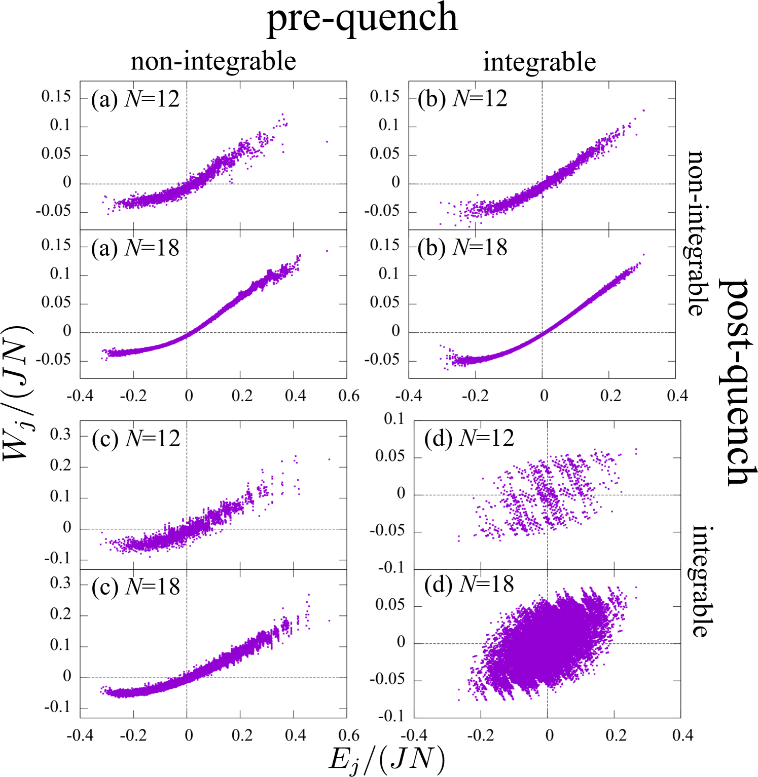
We show our numerical result on the distribution of the extracted work over energy eigenstates. Figure 1 shows versus the eigenenergy . Overall, the average work tends to be negative (positive) in the positive (negative) temperature region.
Specifically, in the case of (a), (b), and (c), where one or both of Hamiltonians and are non-integrable, the distribution of the data points becomes narrower in the horizontal direction from to . We thus expect that these data points converge to a single smooth curve in the thermodynamic limit . This is analogous to the strong ETH Jensen1985 ; Rigol2008 ; Steinigeweg2013 ; Steinigeweg2014 ; Beugeling2014 ; Kim2014 ; Khodja2015 ; Garrison2015 ; Mondaini2016 ; Dymarsky2018 ; Yoshizawa2017 . On the other hand, in the case of (d), the distribution of the data points is more spread out than the other cases and does not look like convergent to a single curve. This is analogous to the behavior of the ETH in integrable systems Rigol2008 ; Biroli2010 .
We also note that in the case of (a), (b), and (c), eigenstates with do not exist in the positive temperature region for , whereas in the integrable case (d), there are work extractable eigenstates also in the positive temperature region.
To confirm the validity of the above argument more quantitatively, we systematically investigate the number of work-extractable energy eigenstates in the next subsection.
II.4 Dependence on size and integrability
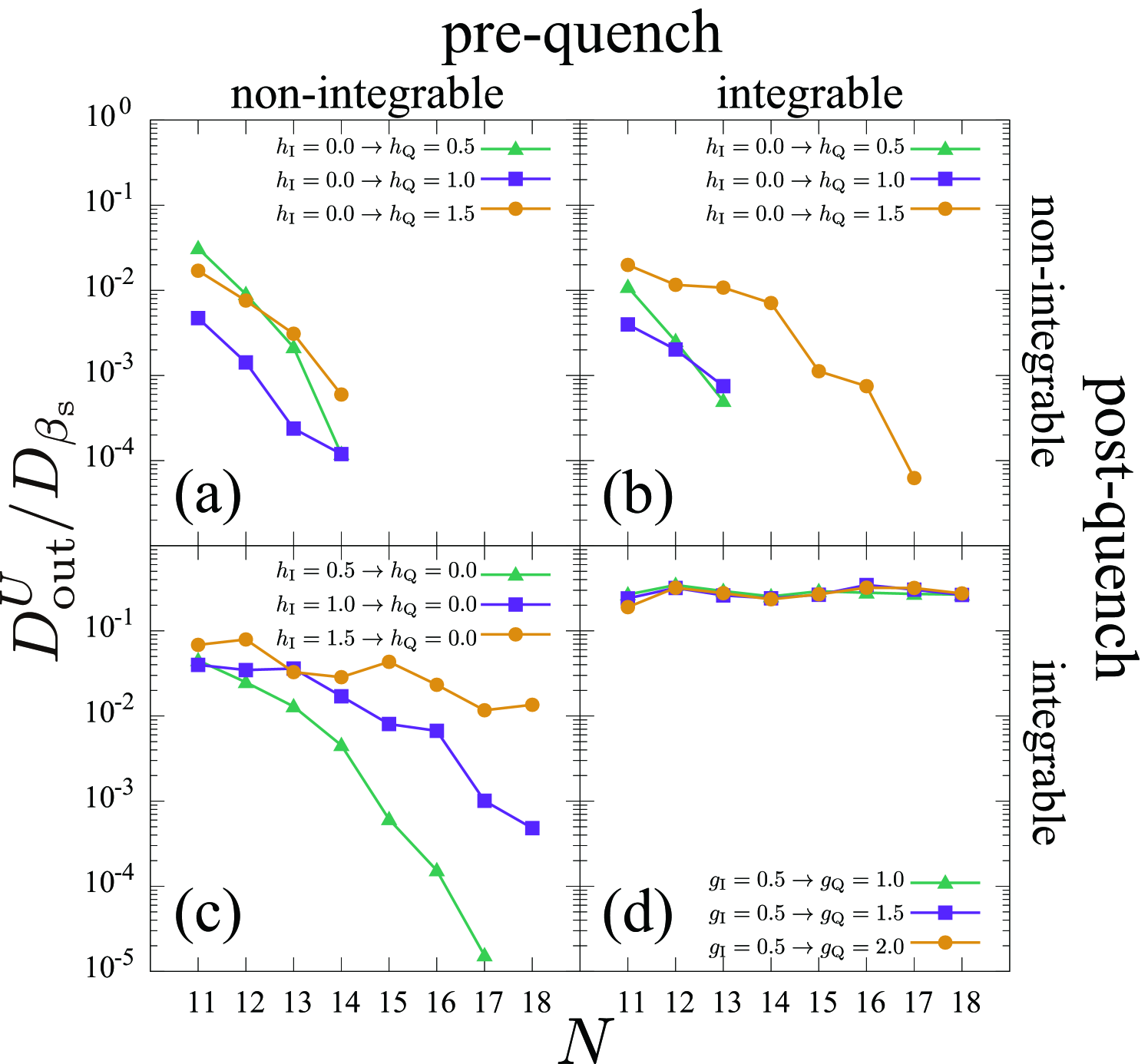
We next quantitatively study the system-size dependence of the number of energy eigenstates from which one can extract positive work. We focus on eigenstates at positive finite temperature . In addition, we set a threshold for the inverse temperature, denoted as , because the finite-size effect is significant in small . The set of energy eigenstates with is denoted by We denote the number of energy eigenstates in by . Let be the number of eigenstates in from which one can extract work greater than (i.e., ). We numerically investigate the system-size dependence of the ratio .
Figure 2 shows the system-size dependence of for several quench protocols. In the case of (a), (b), and (c), where one or both of Hamiltonians and are non-integrable, decays at least exponentially with . On the other hand, does not seem to be decreasing in the case of (d), where both and are integrable. Especially, in the case of (a) and (b), becomes exactly zero even at finite , at which eigenstates with completely vanish. This is regarded as a stronger version of the second law at the level of individual energy eigenstates, which is analogous to the strong ETH.
Apparently, does not seem to be decreasing in the case of (d), where both and are integrable. However, as will be shown in inequality (8), which is applicable to this case, must decrease at least exponentially. This is because the parameters in inequality (8) in our numerical setup are very small ( and ), and therefore the decay rate is too small to be observed in our numerical result. We note that in the case of (d), itself increases exponentially with , because itself increases exponentially. Therefore, does not become exactly zero at finite , which is analogous to the weak ETH in integrable systems Biroli2010 ; Yoshizawa2017 ; Tasaki2015 ; Mori2016 .
Table 1 summarizes whether the stronger version of the second law (i.e., at finite ) holds or not in our numerical calculations. In the case of (c), whether this property holds is not very clear from Fig. 2 (c), due to the limitation of our numerical resource. However, we argue that holds at finite in this case too, from the following discussion and the numerical result in Fig. 3 (c).
| Pre-quench Hamiltonian | |||
|---|---|---|---|
| Non-integrable | Integrable | ||
| Post-quench | Non-integrable | (a) True | (b) True |
| Hamiltonian | Integrable | (c) True | (d) False |
III Eigenstate second law from the strong ETH
We discuss the physical mechanism of on the basis of the strong ETH.
III.1 Eigenstate second law from the strong ETH
We assume that Hamiltonian satisfies the strong ETH for observable , i.e.,
| (4) |
Here, represents the microcanonical average with respect to around the energy .
Under this assumption, the average work extracted from is given by
| (5) |
Meanwhile, the average work from the Gibbs state of at the mean energy is given by
| (6) |
where we used the strong ETH and the concentration of the energy in the Gibbs state Tasaki2018 . We thus obtain , and the passivity of the Gibbs state Pusz1978 ; Lenard1978 (i.e., ) immediately leads to . Therefore, we conclude that for all in the case of (a), (b), and (c), where the strong ETH holds.
III.2 Strong ETH for a non-local observable
We numerically confirm the strong ETH (4). We remark that in general is a non-local observable, which involves products of local operators. The strong ETH for such a non-local many-body observable has not been fully investigated so far.
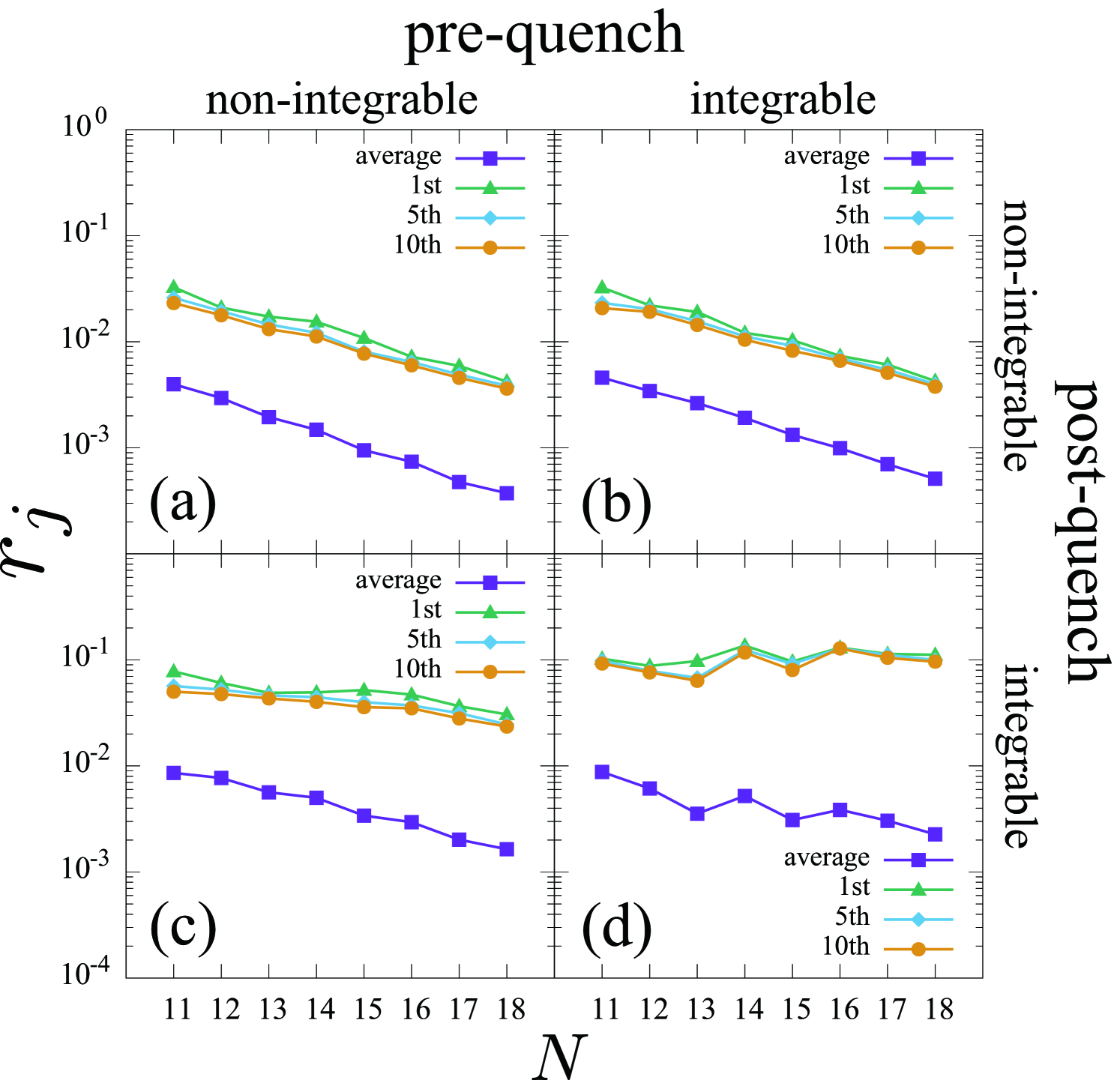
We calculate the ETH indicator , which was introduced in Ref. Kim2014 . Here, is the th energy eigenstate in the increasing order of in the Hilbert space without dividing it into momentum sectors. If the strong ETH holds, all of decay exponentially with . In fact, if there is an athermal eigenstate , the corresponding does not decay. However, even in such a case, the average of decays if the weak ETH holds.
Since we are interested in eigenstates at positive temperature, we remove eigenstates with . We also remove eigenstates at the edge of the spectrum, because the density of states is too small there. Therefore, we calculated for eigenstates satisfying .
Figure 3 shows the system-size dependence of the average, the largest, the fifth largest, and the tenth largest values of . The average of decays exponentially in all the cases, which implies the weak ETH. On the other hand, other values of decay only in the case of (a), (b), and (c), where one or both of Hamiltonians and are non-integrable. These values do not decay in the case of (d) where both and are integrable. Therefore, the strong ETH is valid for the case of (a), (b), and (c), which is consistent with Table 1.
IV General bound on
We make an analytical argument about a general bound on .
IV.1 Assumptions and the statement
We consider a quantum many-body system of spins, and denote the number of energy eigenstates of satisfying by . We then assume that there exists an -independent positive function such that
| (7) |
for any , where , and satisfies in . From the Boltzmann formula Ruelle1999 , is nothing but the entropy density. We also assume that and . These assumptions are indeed provable in rigorous statistical mechanics if the system is translation invariant and the interaction is local Ruelle1999 ; Tasaki2018 .
In this setup, we can show that for an arbitrary fixed unitary operator and arbitrary , the inequality
| (8) |
holds. We show a derivation in the next subsection. Inequality (8) implies that the ratio of energy eigenstates, from which one can extract macroscopic work, decays at least exponentially with the system size. This bound holds for both integrable and non-integrable systems, as long as the aforementioned assumptions are satisfied.
We also remark a similarity between the above argument and the weak ETH, which states that the ratio of athermal eigenstates decays at least exponentially with the system size Yoshizawa2017 ; Tasaki2015 ; Mori2016 . Despite this similarity, the logic behind inequality (8) is different from that behind the weak ETH, as seen in the derivation of inequality (8).
IV.2 Derivation of a general bound on
We now derive inequality (8). We first consider a slightly different quantity from , denoted by , and prove a rigorous bound on . Then, inequality (8) is approximately derived as a corollary.
First of all, we define the stochastic work Esposito2009 ; Campisi2011 ; Sagawa2012 . We perform projective measurements of before and after the operation , which give outcomes and , respectively. The stochastic work is defined as the difference between the measured energies: . If the initial density operator is , the joint probability of observing such outcomes is .
For a given positive constant , the probability that we extract work larger than is given by , where is the step function, i.e., and . Here, is the probability of extracting macroscopic work, as is proportional to the system size. For an energy eigenstate, the probability of extracting macroscopic work is . If is sufficiently small for a small , we cannot extract macroscopic work from the energy eigenstate .
We consider the number of energy eigenstates in , from which we can extract macroscopic work by a fixed operation . We focus on the energy eigenstate with which decays exponentially with . In other words, its energy distribution after the protocol shows the large deviation behavior Touchette2009 , and the probability of observing lower energy than the initial state is negligibly small on a macroscopic scale. Then, we denote by the number of energy eigenstates whose is greater than :
| (9) |
We note that is negligibly small for large , which corresponds to the second law as work extraction.
In this setup, we can rigorously prove the following inequality:
| (10) |
The proof of this inequality is as follows. From the definition of , we have
| (11) |
We can evaluate the sum in the right-hand side by using the definition of as
| (12) | |||
| (13) | |||
| (14) | |||
| (15) |
where we used to obtain the fourth line. From the assumption (7), we obtain
| (16) |
Meanwhile, and imply . Therefore, we have
| (17) |
By combining this inequality and inequality (15), we have
| (18) |
which implies inequality (10).
The definition of is slightly different from . For the latter, we can only obtain an approximate inequality (8) as follows. If , the average work extraction from is bounded as
| (19) | ||||
| (20) | ||||
| (21) |
From this inequality, we have . Therefore, we obtain
| (22) |
IV.3 Work extraction from a general pure state
From inequality (8), we can show that a positive amount of work cannot be extracted from any pure state if it has sufficiently large effective dimensions. We consider a general pure state in the Hilbert space of positive temperature region, i.e., with . We apply the general work extraction protocol in Sec. IV.2 to .
The probability of extracting macroscopic work from is . The Cauchy-Schwartz inequality gives
| (23) | |||
| (24) | |||
| (25) |
where we used inequality (10) to obtain the third line and defined the effective dimension Reimann2008 . From this inequality, the average work extraction from is bounded as
| (26) | ||||
| (27) |
where is the maximum value of the stochastic work. scales at most linearly with .
Therefore, holds for any unitary operation, if the initial state has sufficiently large effective dimensions: . Because the effective dimension of a typical pure state with respect to the Haar measure is estimated as Linden2009 , we cannot extract macroscopic work from a typical pure state.
V Conclusion
In this paper, we have investigated work extraction from a single energy eigenstate by a specific cyclic operation and clarified the effect of the integrability on work extraction. Our main numerical results are presented in Fig. 2 and Table 1.
Roughly speaking, work extraction by our quench protocol is impossible from any energy eigenstate if the system is non-integrable, while it is impossible from most energy eigenstates if the system is integrable. We thus conjecture that the same result would hold for a much broader class of physical work extraction protocols with local and translation invariant Hamiltonians. This is in fact feasible in light of the fact that the strong ETH has been confirmed to be true for a broad class of Hamiltonians Jensen1985 ; Rigol2008 ; Steinigeweg2013 ; Steinigeweg2014 ; Beugeling2014 ; Kim2014 ; Khodja2015 ; Garrison2015 ; Mondaini2016 ; Dymarsky2018 ; Yoshizawa2017 . If the above conjecture is true, we can conclude that the second law is so universal that it applies at the level of individual energy eigenstates. Further investigation of this conjecture is a future issue.
On the other hand, in many-body localization systems (MBL) without translation invariance Altman2014 ; Nandkishore2015 ; Abanin2018 , not only the strong ETH but also the weak ETH fails Pal2010 ; Imbrie2016 . The possibility of work extraction from such an exotic system is an interesting direction for future investigation.
Acknowledgements.
K.K. is grateful to K. Yamaga for valuable discussions. K.K. are supported by JSPS KAKENHI Grant Number JP17J06875. E.I. and T.S. are supported by JSPS KAKENHI Grant Number JP16H02211. E.I. is also supported by JSPS KAKENHI Grant Number JP15K20944.Appendix A Level statistics
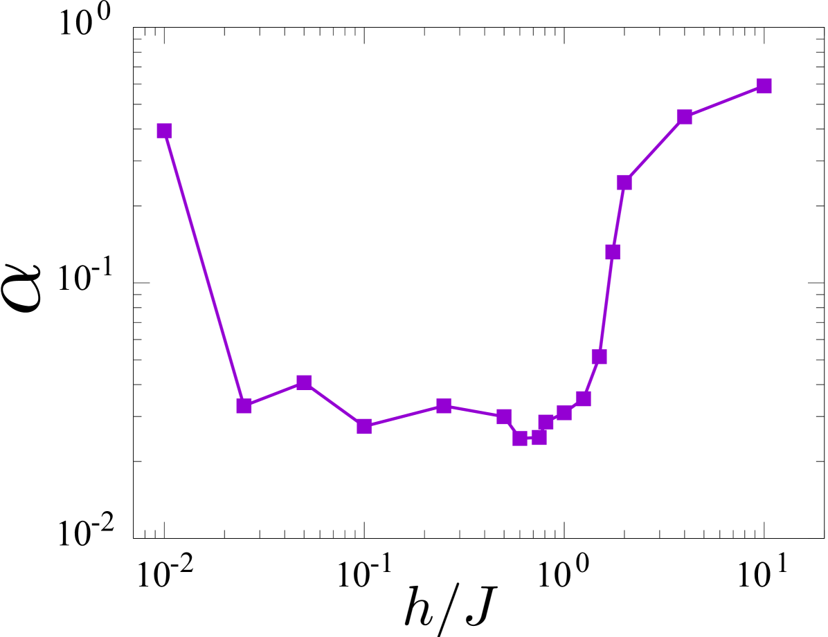
In order to confirm that the parameters chosen in the numerical calculation have sufficient non-integrability, we investigate the level spacing statistics. In particular, we calculated the ratio of adjacent energy gap Oganesyan2007 which is defined as . Here, is the gap between the eigenenergies, and the eigenenergies are listed in increasing order in each momenta sector. If the system is nonintegrable, follows the Wigner-Dyson distribution given by random matrix theory. For the system with time-reversal symmetry, the distribution is well fitted by the Gaussian orthogonal ensemble (GOE), whose explicit form in our formulation is given by Atas2013 :
| (28) |
By numerical exact diagonalization, we obtained the distributions of for all the momentum sectors, except for and . We denote the average distribution of over these momentum sectors by . We consider an indicator of the distance between and Santos2010 :
| (29) |
where is the size of a bin used in our calculation of . This indicator is expected to be small if the system is sufficiently non-integrable.
Appendix B The time dependence of the average work
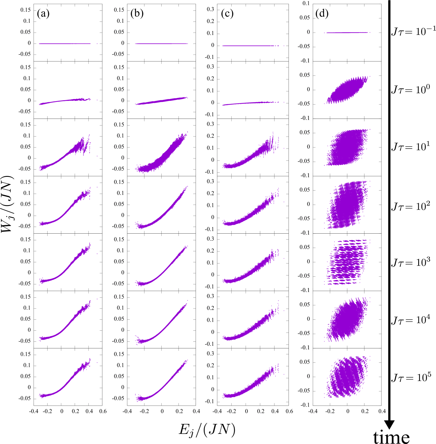
We consider the dependence of the average work on the waiting time in the protocol of Fig. 1. In the following, (a), (b), (c), (d) indicate the four cases of the integrability, as defined in Sec. II . Figure 5 shows the average work per qubit for the full spectrum for various . For , is almost zero for all the cases and takes a non-zero value after . takes an almost constant value up to temporal fluctuations after . The temporal fluctuations are small for the three cases (a), (b), and (c), and the appearances of the scatter plots of are almost the same for . On the other hand, the temporal fluctuations are larger in the case of (d), and the appearances of the scatter plots are not the same for .
Appendix C The parameter-dependence of
In this Appendix, we show the parameter-dependence of . We change only one parameter at once and fix the other parameters to the same value as in Fig. 2. The parameters used in Fig. 2 are given by , and .
C.1 The -dependence
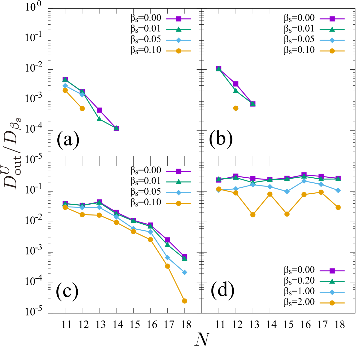
Figure 6 shows the -dependence of . For the two cases (a) and (b), where is non-integrable, vanishes at finite regardless of . In the case of (c), with large decays faster, whereas in the case of (d), we do not observe the decay of .
C.2 The -dependence
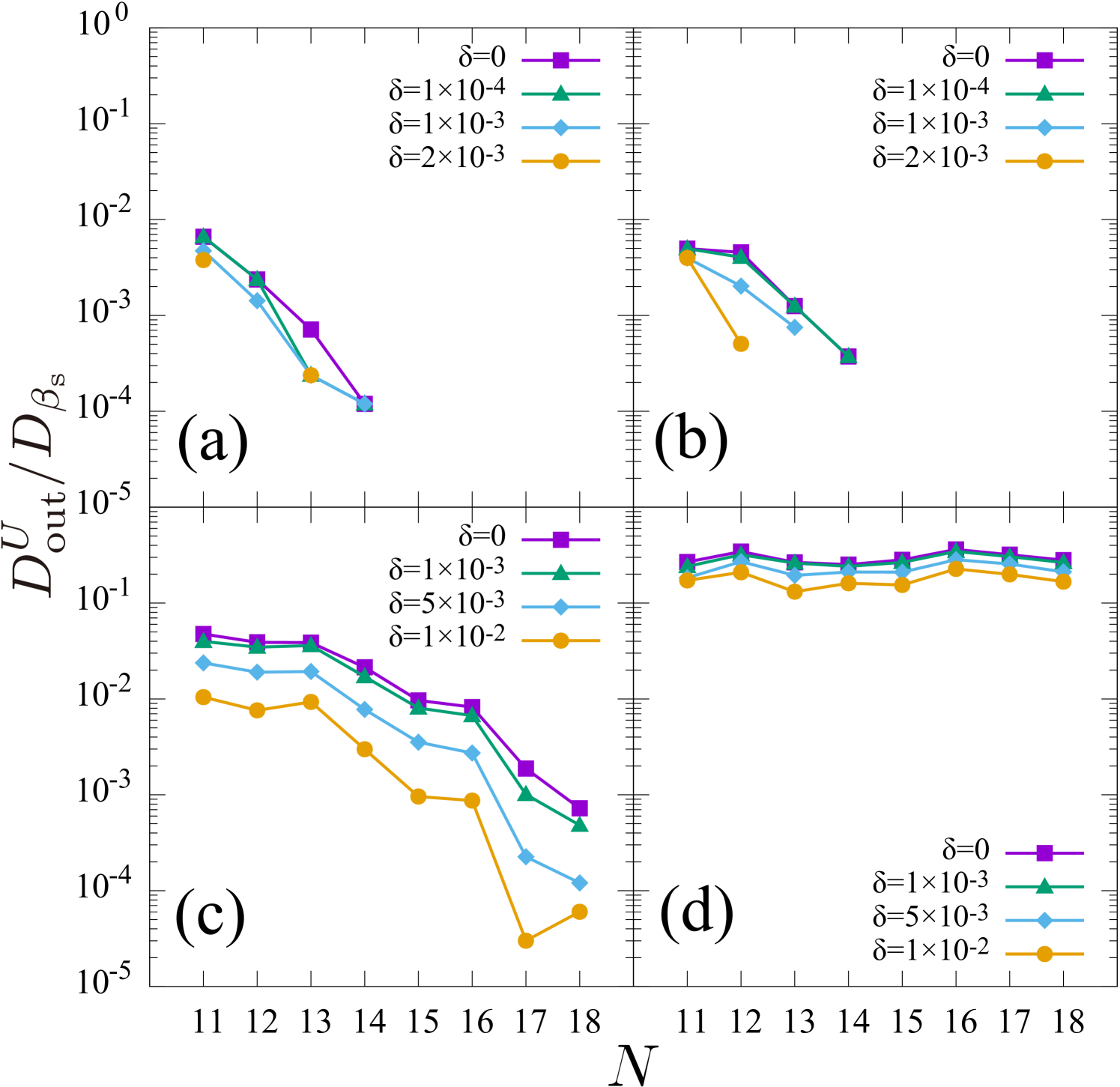
Figure 7 shows the -dependence of . For the two cases (a) and (b), vanishes at finite regardless of . In the case of (c), with large decays faster, and also vanishes at finite when . However, in the case of (d), does not vanish with any .
C.3 Summary
From the above results, we conclude that our statement in the main text is independent of the choice of the parameters: vanishes at finite for (a) and (b) and does not vanishes for (d). The case of (c) is marginal, which is again consistent with our argument in the main text.
References
- (1) H. Tasaki, arXiv:cond-mat/0009206 (2000).
- (2) A. E. Allahverdyan and T. M. Nieuwenhuizen, Phys. A 305, 542 (2002).
- (3) W. Pusz and S. L. Woronowicz, Comm. Math. Phys. 58, 273 (1978).
- (4) A. Lenard, J. Stat. Phys. 19, 575 (1978).
- (5) A. Polkovnikov, K. Sengupta, A. Silva, and M. Vengalattore, Rev. Mod. Phys. 83, 863 (2011).
- (6) L. D’Alessio, Y. Kafri, A. Polkovnikov, and M. Rigol, Adv. Phys. 65, 239 (2016).
- (7) J. Eisert, M. Friesdorf, and C. Gogolin, Nat. Phys. 11, 124 (2015).
- (8) C. Gogolin and J. Eisert, Rep. Prog. Phys. 79, 056001 (2016).
- (9) M. V. Berry, J. Phys. A 10, 2083 (1977).
- (10) A. Peres, Phys. Rev. A 30, 504 (1984).
- (11) J. M. Deutsch, Phys. Rev. A 43, 2046 (1991).
- (12) M. Srednicki, Phys. Rev. E 50, 888 (1994).
- (13) M. Rigol, V. Dunjko, and M. Olshanii, Nature (London) 452, 854 (2008).
- (14) R. V. Jensen and R. Shankar, Phys. Rev. Lett. 54, 1879 (1985).
- (15) R. Steinigeweg, J. Herbrych, and P. Prelovŝek, Phys. Rev. E 87, 012118 (2013).
- (16) R. Steinigeweg, A. Khodja, H. Niemeyer, C. Gogolin, and J. Gemmer, Phys. Rev. Lett. 112, 130403 (2014).
- (17) W. Beugeling, R. Moessner, and M. Haque, Phys. Rev. E 89, 042112 (2014).
- (18) H. Kim, T. N. Ikeda, and D. A. Huse, Phys. Rev. E 90, 052105 (2014).
- (19) A. Khodja, R. Steinigeweg, and J. Gemmer, Phys. Rev. E 91, 012120 (2015).
- (20) R. Mondaini, K. R. Fratus, M. Srednicki, and M. Rigol, Phys. Rev. E 93, 032104 (2016).
- (21) J. R. Garrison and T. Grover, Phys. Rev. X 8, 021026 (2018).
- (22) A. Dymarsky, N. Lashkari, and H. Liu, Phys. Rev. E 97, 012140 (2018).
- (23) T. Yoshizawa, E. Iyoda, and T. Sagawa, Phys. Rev. Lett. 120, 200604 (2018).
- (24) M. Rigol, Phys. Rev. Lett. 103, 100403 (2009).
- (25) G. Biroli, C. Kollath, and A. M. Läuchli, Phys. Rev. Lett. 105, 250401 (2010).
- (26) V. Alba, Phys. Rev. B 91, 155123 (2015).
- (27) F. H. L. Essler and M. Fagotti, J. Stat. Mech. 064002 (2016).
- (28) L. Vidmar and M. Rigol, J. Stat. Mech. 064007 (2016).
- (29) H. Tasaki, J. Stat. Phys. 163, 937 (2016).
- (30) T. Mori, arXiv:1609.09776 (2016).
- (31) E. Iyoda, K. Kaneko, and T. Sagawa, Phys. Rev. Lett. 119, 100601 (2017).
- (32) H. Tasaki, arXiv:cond-mat/0011321 (2000).
- (33) S. Goldstein, T. Hara, and H. Tasaki, arXiv:1303.6393 (2013).
- (34) T. N. Ikeda, N. Sakumichi, A. Polkovnikov, and M. Ueda, Ann. Phys. (Amsterdam) 354, 338 (2015).
- (35) K. Kaneko, E. Iyoda, and T. Sagawa, Phys. Rev. E 96 062148 (2017).
- (36) R. Dorner, S. R. Clark, L. Heaney, R. Fazio, J. Goold, and V. Vedral, Phys. Rev. Lett. 110, 230601 (2013).
- (37) R. Gallego, A. Riera, and J. Eisert, New J. Phys. 16, 125009 (2014).
- (38) M. Perarnau-Llobet, A. Riera, R. Gallego, H. Wilming, and J. Eisert, New J. Phys. 18, 123035 (2016).
- (39) R. Modak and M. Rigol, Phys. Rev. E 95, 062145 (2017).
- (40) T. P. Le, J. Levinsen, K. Modi, M. M. Parish, and F. A. Pollock, Phys. Rev. A 97, 022106 (2018).
- (41) F. Jin, R. Steinigeweg, H. De Raedt, K. Michielsen, M. Campisi, and J. Gemmer, Phys. Rev. E 94, 012125 (2016).
- (42) D. Schmidtke, L. Knipschild, M. Campisi, R. Steinigeweg, and J. Gemmer, Phys. Rev. E 98, 012123 (2018).
- (43) S. Trotzky, Y-A. Chen, A. Flesch, I. P. McCulloch, U. Schollwöck J. Eisert, and I. Bloch, Nat. Phys. 8, 325 (2012).
- (44) T. Langen, S. Erne, R. Geiger, B. Rauer, T. Schweigler, M. Kuhnert, W. Rohringer, I. E. Mazets, T. Gasenzer, and J. Schmiedmayer, Science 348, 207 (2015).
- (45) C. Neill, P. Roushan, M. Fang, Y. Chen, M. Kolodrubetz, Z. Chen, A. Megrant, R. Barends, B. Campbell, B. Chiaro, A. Dunsworth, E. Jeffrey, J. Kelly, J. Mutus, P. J. J. O’Malley, C. Quintana, D. Sank, A. Vainsencher, J. Wenner, T. C. White, A. Polkovnikov, and J. M. Martinis, Nat. Phys. 12, 1037 (2016).
- (46) D. Ruelle, Statistical Mechanics: Rigorous Results (World Scientific, Singapore, 1999).
- (47) H. Tasaki, J. Stat. Phys. 172, 905 (2018).
- (48) M. Esposito, U. Harbola, and S. Mukamel, Rev. Mod. Phys. 81, 1665 (2009).
- (49) M. Campisi, P. Hänggi, and P. Talkner, Rev. Mod. Phys. 83, 771 (2011).
- (50) T. Sagawa, Lect. Quantum Comput. Thermodyn. Stat. Phys. 8, 127 (2012).
- (51) H. Touchette, Phys. Rep. 478, 1 (2009).
- (52) P. Reimann, Phys. Rev. Lett. 101, 190403 (2008).
- (53) N. Linden, S. Popescu, A. J. Short, and A. Winter, Phys. Rev. E 79, 061103 (2009).
- (54) R. Nandkishore and D. A. Huse, Annu. Rev. Condens. Matter Phys. 6, 15 (2015).
- (55) E. Altman and R. Vosk, Annu. Rev. Condens. Matter Phys. 6, 383 (2015).
- (56) D. A. Abanin, E. Altman, I. Bloch, and M. Serbyn, arXiv:1804.11065 (2018).
- (57) A. Pal and D. A. Huse, Phys. Rev. B 82, 174411 (2010).
- (58) J. Z. Imbrie, J. Stat. Phys. 163, 998 (2016).
- (59) V. Oganesyan and D. A. Huse, Phys. Rev. B 75, 155111 (2007).
- (60) Y. Y. Atas, E. Bogomolny, O. Giraud, and G. Roux, Phys. Rev. Lett. 110, 084101 (2013).
- (61) L. F. Santos and M. Rigol, Phys. Rev. E 81, 036206 (2010).