Worlds Next Door: A Candidate Giant Planet Imaged in the Habitable Zone of Cen A.
I. Observations, Orbital and Physical Properties, and Exozodi Upper Limits
Abstract
We report on coronagraphic observations of the nearest solar-type star, Cen A, using the MIRI instrument on the James Webb Space Telescope. The proximity of Cen (1.33 pc) means that the star’s habitable zone is spatially resolved at mid-infrared wavelengths, so sufficiently large planets or quantities of exozodiacal dust would be detectable via direct imaging. With three epochs of observation (August 2024, February 2025, and April 2025), we achieve a sensitivity sufficient to detect 225–250 K (1–1.2 ) planets between 1″–2″ and exozodiacal dust emission at the level of 5–8 the brightness of our own zodiacal cloud. The lack of exozodiacal dust emission sets an unprecedented limit of a few times the brightness of our own zodiacal cloud—a factor of 5–10 more sensitive than measured toward any other stellar system to date. In August 2024, we detected a Fν(15.5 m) = 3.5 mJy point source, called , at a separation of 1.5″ from Cen A at a contrast level of . Because the August 2024 epoch had only one successful observation at a single roll angle, it is not possible to unambiguously confirm as a bona fide planet. Our analysis confirms that is neither a background nor a foreground object. is not recovered in the February and April 2025 epochs. However, if is the counterpart of the object, , seen by the VLT/NEAR program in 2019, we find that there is a 52% chance that the candidate was missed in both follow-up JWST/MIRI observations due to orbital motion. Incorporating constraints from the non-detections, we obtain families of dynamically stable orbits for with periods between 2–3 years. These suggest that the planet candidate is on an eccentric () orbit significantly inclined with respect to the Cen AB orbital plane (, prograde, or , retrograde). Based on the photometry and inferred orbital properties, the planet candidate could have a temperature of 225 K, a radius of 1–1.1 and a mass between 90–150 , consistent with RV limits. This paper is first in a series of two papers: Paper II (Sanghi & Beichman et al. 2025, in press) discusses the data reduction strategy and finds that is robust as a planet candidate, as opposed to an image or detector artifact.
show]chas@ipac.caltech.edu
show]asanghi@caltech.edu
1 Introduction
Centauri A is the closest solar-type star to the Sun and offers a unique opportunity for direct imaging with the James Webb Space Telescope (JWST) to detect an exoplanet within its habitable zone and to achieve an unprecedented level of sensitivity for the detection of an exozodiacal dust cloud (Beichman et al., 2020; Sanghi et al., 2025). Among the nearby stars, Cen A, primus inter pares, offers a nearly 3-fold improvement in the angular scale of its Habitable Zone and a 7.5-fold boost in the absolute brightness of any planet compared to the next nearest solar type star, Ceti. Specifically, the F1550C coronagraph onboard the Mid-InfraRed Instrument (MIRI) can be used to probe the 1–3 au (4″) region around Cen A which is predicted to be stable within the Cen AB system for exoplanets and/or an exozodiacal dust cloud (Quarles, Lissauer & Kaib, 2018; Cuello & Sucerquia, 2024). The detection of a planet or exozodiacal emission, or more stringent limits on either, would advance our understanding of the formation of planetary systems in binary stellar systems and yield an important target for future observations with both JWST and the extremely large ground-based telescopes. Of particular interest is the ability of JWST/MIRI to confirm the detection of a candidate () identified using the VISIR mid-infrared camera (10–12.5 m) on ESO’s Very Large Telescope (VLT) as part of the NEAR (New Earths in Alpha Centauri Region) Breakthrough Watch Project (Wagner et al., 2021).
In this paper, we present the results of a deep search for planets and zodiacal dust emission obtained with three epochs of JWST/MIRI coronagraphic imaging observations of Cen A. This paper is the first in a series and is followed by Sanghi & Beichman et al. (2025, also referred to as Paper II). It is organized as follows. Section 2 describes the observational strategy and program execution. Section 3 summarizes key aspects of the data processing strategy, the detection of a candidate exoplanet in the August 2024 data, the planet temperature sensitivity of our observations, and upper limits on the presence of exozodiacal emission. Section 4 analyzes possible orbital configurations for the candidate planet. The planet’s physical properties, as constrained by its observed brightness and orbit, as well as by radial velocity measurements (Wittenmyer et al., 2016; Zhao et al., 2018), are considered in Section 5. Section 6 discusses the importance of the presence of the candidate planet and the upper limits on exozodiacal emission in the context of theories of planet and disk formation in binary systems, as well as prospects for recovering the candidate in future observations. Finally, Section 7 presents our conclusions. Appendix A provides the complete details of observation preparation and Appendix B includes new ALMA astrometry and an updated ephemeris for the Cen AB system.
2 Observations
| Property | Cen A | Cen B | Mus | References |
|---|---|---|---|---|
| Spectral Type | G2V | K1V | M4III | 1, 2 |
| Mass () | 1.0788 0.0029 | 0.9092 0.0025 | 3 | |
| Luminosity () | 1.5059 0.0019 | 0.4981 0.0007 | 3 | |
| (mag) | 1.48 0.05 | 0.60 0.05 | 1.42 0.05 | 2, 4 |
| F1065C | (160 Jy) | (51 Jy) | (194 Jy) | 5, 6, 7 |
| F1140C | (120 Jy) | (59 Jy) | (180 Jy) | 5, 6, 7 |
| F1550C | (63 Jy) | (28 Jy) | (100 Jy) | 5, 6, 7 |
| Parallax (mas) | 3, 8 | |||
| Distance (pc) | 1.33 | 100 | 3, 8 | |
| Proper Motion (, mas yr-1) | (, ) | (, ) | 3, 8 | |
| R.A. | 14:39:26.155 | 14:39:25.9421 | 12:17:33.620 | 3, 8, 9 |
| Decl. | 60:49:56.287 | 60:49:51.334 | 67:57:39.072 | 3, 8, 9 |
References. — (1) Valenti & Fischer (2005); (2) Ducati (2002); (3) Akeson et al. (2021); (4) Engels et al. (1981); (5) from angular size of Cen A, mas combined with a Kurucz-Castelli model with K and log dex (cgs units; Kervella et al., 2017); (6) From fit to Kurucz model atmosphere using VOSA SED utility (Engels et al., 1981; Ducati, 2002; Castelli & Kurucz, 2003; Bayo et al., 2008); (7) Olnon et al. (1986); (8) Gaia Collaboration et al. (2016); (9) for Mus Epoch 2016.0 (Gaia DR3) and for Cen Epoch 2019.5 (Akeson et al., 2021).
2.1 Observational Strategy
We elected to observe with MIRI and its Four Quadrant Phase Mask Coronagraph (4QPM; Rieke et al., 2015; Wright et al., 2015; Boccaletti et al., 2022) centered at 15.5 m (the F1550C filter) for a number of reasons: (1) favorable star-planet contrast ratio for the 200–350 K temperatures expected for a planet heated by Cen A at 1–3 au; (2) low susceptibility to the effects of wavefront drift at this long wavelength; and (3) the reduced brightness of background objects with typical stellar photospheres. However, despite these advantages, the Cen AB system presents numerous challenges in planning and executing coronagraphic measurements with JWST at any wavelength.
-
•
The presence of Cen B only 7″–9″ away from Cen A puts the full intensity of this bright, [F1550C] mag star in the focal plane at a position that cannot be attenuated. We developed a strategy (A.4) to place Mus at the position Cen B would occupy (unocculted) during the observation of Cen A (occulted). This observation would provide a PSF reference to mitigate the effects of Cen B.
-
•
The selection of a reference star is complicated by the requirement that it be both comparably bright to Cen A and have similar photospheric properties in the F1550C waveband.
-
•
The moment-by-moment position of Cen A is the result of a complex interplay of its high proper motion and parallax (as calculated for the location of JWST at the epoch of observation), and of the orbital motion of Cen A and Cen B about their common center of mass (see Akeson et al., 2021, and Table 2).
-
•
With [F1550C] mag, Cen A is too bright for direct target acquisition (TA) with MIRI, necessitating a blind offset from a nearby star with an accuracy of 10 mas to avoid degradation of the coronagraphic contrast (Boccaletti et al., 2015). The chosen reference star Mus (A.1) is similarly too bright for direct TA, also necessitating a blind offset.
-
•
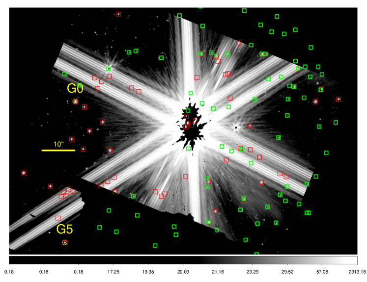
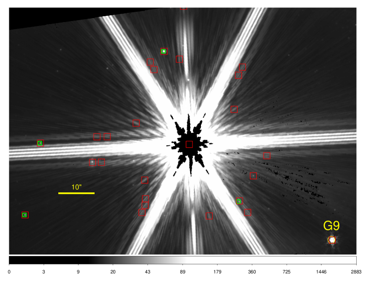
Offset stars must be of sufficient astrometric accuracy, be as close as possible to Cen A or Mus, but not affected by diffraction or other artifacts from the target stars, and be of sufficient brightness to be readily detectable in a short TA observation at F1000W (Figure 1).
-
•
The time of observation should minimize the change in solar aspect angle between target and reference star observations and thus minimize the change in the telescope’s thermal environment.
-
•
Finally, all MIRI coronagraphic observations using the 4QPM are affected by excess background radiation appearing around the quadrant boundaries referred to as the “Glow Sticks” (Boccaletti et al., 2022).
2.2 Planned Observation Sequences
The above considerations led to the observational sequences described below and detailed in Appendix A. Based on in-flight performance, JWST can place both the target and reference star with an accuracy of 5–7 mas (1, each axis) behind the MIRI/4QPM. To provide diversity in determining the PSF for post-processing, we selected a 9-point dither pattern for observing the reference star. The multiple reference PSF observations improve the ability of post-processing algorithms to remove residual stellar speckles and help to mitigate wavefront error (WFE) drifts over the 32 hr duration of the entire sequence. The measurement strategy was as follows:
-
1.
Offset from a Gaia star ( in Figure 1) to place Mus at the center of the F1550C coronagraphic mask and make a 9-point dithered set of image observations This is followed by observations of a background field to subtract the Glow Stick.
-
2.
Place Mus at the detector location that Cen B would occupy in the Roll #1 observation to help mitigate speckles from the unocculted star at the position of Cen A.
-
3.
Offset from a Gaia star ( or in Figure 1) to place Cen A at the center of the F1550C coronagraphic mask at the Roll #1 V3PA111V3PA is the position angle (PA) of the V3 reference axis eastward relative to north when projected onto the sky. angle for a sequence of 1250 images, followed by observations of a background field to subtract the Glow Stick.
-
4.
Repeat the Cen A sequence (#3) at a second V3PA angle (Roll #2).
-
5.
Repeat the Mus 9-point dither sequence (#1) at the mask center.
-
6.
Repeat the off-axis Mus observation sequence (#2) but at the detector position of Cen B in the Roll #2 observation.
2.3 Executed Observation Sequences
The observations of Cen A (Cycle 1 GO, PID #1618; PI: Beichman, Co-PI: Mawet) were initiated in August 2023, but were unsuccessful due to target acquisition and offset failures. A sequence of short test images was obtained in June and July 2024 to validate the target acquisition strategy. Specifically, in July 2024, we executed #1 without dithering and #3 with fewer integrations.222No Mus reference star observation was acquired at the detector position of Cen B in the July 2024 test observations. This severely compromised the quality of PSF subtraction. Hence, these observations are not presented. Following successful execution of the test program, we conducted our full-set of science observations in August 2024. We successfully executed steps #1, #4, and #6 (#2 was not part of the sequence planned for this observation). However, the first roll on Cen A (#3) and the second Mus observation (#5) were unsuccessful due to guide star failures.
Based on results from the August 2024 data, the STScI Director’s Office approved a follow-up Director’s Discretionary Time (DDT) program (PID #6797; PI: Beichman, Co-PI: Sanghi). The complete two roll sequence with associated reference star observations (#1–#6) was attempted in February 2025 as part of this DDT program, but due to a telescope pointing anomaly, the first Cen A roll (#3) was not executed. All other observations were successful.
The STScI Director’s Office approved a second follow-up DDT program (PID #9252; PI: Beichman, Co-PI: Sanghi), which resulted in the successful execution of a full two roll sequence in April 2025. A summary log of all successful observations is provided in Table 8. In all cases, the accuracy of the offsets from Gaia stars was consistent with the expected initial pointing accuracy (, 5–7 mas), the offset accuracy (, 1.5 mas) and the line-of-sight jitter (, 1.5 mas) during the observing sequence at each position. The February 2025 Roll 2 and April 2025 Roll 1 observations showed offsets of 10 mas from the 4QPM center or from the Eps Mus dither pattern and were thus of lower quality (see dither map in Sanghi & Beichman et al., 2025).
| ID | Epoch | (, ) | ( | Wavelength | Flux | Contrast | S/N |
|---|---|---|---|---|---|---|---|
| (″) | (″, ∘) | (m) | (mJy) | to Cen A | |||
| June 1, 2019 | ( 0.05 | (0.85 0.05, 228.9 3.3) | 11.25 | 1.2 0.4 | 3 | ||
| August 10, 2024 | (1.50, 0.17) 0.13 | (1.51 0.13, 83.5 4.9) | 15.5 | 3.5 1.0 | 4–6 |
Note. — Observations of were obtained in 2019 by the VLT/NEAR experiment Wagner et al. (2021). Position angle () is measured East of North.
3 Results
3.1 Summary of Data Reduction
Paper II (Sanghi & Beichman et al., 2025) describes in detail the initial pipeline processing, PSF subtraction techniques for both Cen A and Cen B, source identification steps, the photometry and astrometry estimation procedures, and detection sensitivity analysis. Here, we provide a short summary. Level 0 data products were downloaded from MAST, processed for best up-the-ramp calculation of source brightness and bad pixel rejection (Brandt, 2024; Carter et al., 2025), and post-processed to remove the residual stellar diffraction from Cen A and Cen B. We assembled distinct reference PSF libraries for each epoch consisting of the individual 400 frames (per dither position) of each 9-pt SGD observation of Mus behind the 4QPM and the individual 1250 frames of Mus at the unocculted position of Cen B (for a given roll) obtained at the corresponding epoch. We employed reference star differential imaging (RDI) and jointly subtracted Cen AB from the 1250 Cen integrations using the principal component analysis-based Karhunen-Loève Image Processing algorithm (Soummer et al., 2012). Signal-to-noise ratio maps were generated to search for point sources (Mawet et al., 2014) and extended emission (custom method), and assess detection significance.
3.2 Detection of a Point Source Around Cen A
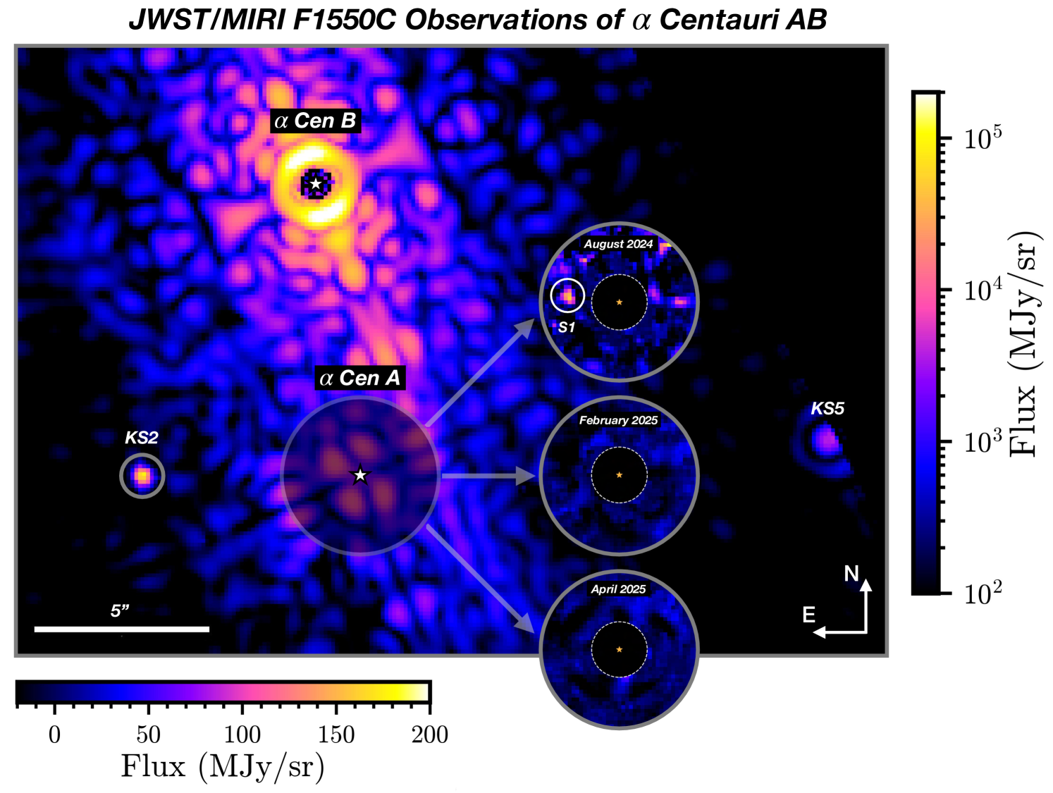
A comprehensive search of the 3″ region around Cen A revealed a single point-like source in the August 2024 data, (Figure 2). The source was detected 15 East of Cen A at a S/N between 4–6 (corresponding to a 3.3–4.3 Gaussian significance for the equivalent false positive probability, see Paper II) with a flux density of mJy (Table 2). The contrast of with respect to Cen A in the F1550C bandpass is . is not recovered in the February and April 2025 observations (Figure 2). At wider separations, in all three epochs, we identified two objects denoted KS2 and KS5 that are known from deep 2 m VLT/NACO imaging to be background stars (Kervella et al., 2016). In the August 2024 data, KS2 is seen ″ East of Cen A, after post-processing, exactly in the position expected for a distant, low proper motion star (Figure 2). The bright object KS5 ( mag) is detected just off the edge of the coronagraphic field and will eventually pass within a few mas of Cen A (mid-2028; Kervella et al., 2016).
Paper II (Sanghi & Beichman et al., 2025) discusses the robustness of the detection of and with the help of several tests, presents reasonable evidence that is a celestial signal, as opposed to an image artifact. Three primary artifact scenarios are shown to be unlikely:
-
•
is not likely a short-lived detector artifact in the Cen AB integrations. was independently detected in multiple subsets of the full 1250 frame integration sequence . Additionally, there was no evidence for transient “hot pixels” in the data, centered on .
-
•
is not likely a PSF-subtraction artifact from the Mus coronagraphic reference images. was detected in post-processing analyses performed by iteratively excluding each one of the nine dither positions (“leave-one-out” analysis, .
-
•
is not likely a PSF-subtraction artifact from imperfect subtraction of Cen B. is well matched to the expected PSF profile and behaves differently with respect to changes in subtraction parameters from another point-like object () identified as an artifact from Cen B.
To assess whether is physically associated with Cen A, we address whether it could be either a background or foreground (Solar System) object. Multiple arguments rule out these scenarios:
-
•
First and most conclusively, the JWST data themselves provide definitive evidence against the hypothesis that is a background object. No point source counterparts to are detected at the expected location for a background source in the February 2025 and April 2025 observations (Figure 3). See Paper II (Sanghi & Beichman et al., 2025) for further details.
-
•
Archival images taken by Spitzer/IRAC (Rieke & Gautier, 2004), 2MASS, and VLT/NACO (Kervella et al., 2016) when Cen A was up to one arcminute away from its current position do not show any sources at the position. We also considered the effects of interstellar extinction on background source detectability in archival imaging. Extinction maps from Planck and stellar data along the line-of-sight toward Cen provide a range (Planck Collaboration et al., 2016; Zhang & Kainulainen, 2022), making more extreme values unlikely.333Planck Extinction maps:
https://irsa.ipac.caltech.edu/data/Planck/release_2/all-sky-maps/maps/component-maps/foregrounds/COM_CompMap_Dust-DL07-AvMaps_2048_R2.00.fits As shown in Figure 4, if were a reddened star (an M0III Kurucz model with K is shown; Buser & Kurucz, 1992) or a normal star-dominated galaxy, its emission would be 4 to 25 times brighter at IRAC wavelengths than at F1550C and would have been detectable by Spitzer, or in the deep NACO -band image. This argument applies to any stellar temperature, since at these wavelengths the emission is approximately Rayleigh-Jeans. -
•
Figure 4 also shows the spectral energy distribution for a non-photosphere dominated galaxy, the prototypical starburst galaxy or ULIRG, Arp 220, at zero redshift (Polletta et al., 2007). Such an object could have escaped detection in the archival datasets, but the probability of chance alignment with an extragalactic background object is extremely low based on source-counting studies in the MIRI broadband filters. Stone et al. (2024) find that the background density of 1 mJy sources is 0.05 arcmin-2, corresponding to a chance alignment likelihood within a 3″ field-of-view.
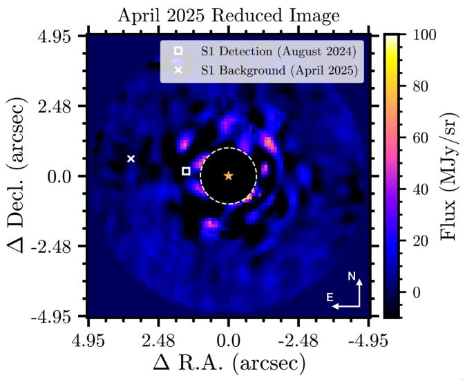
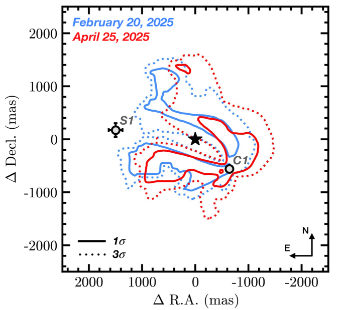
Figure 3: PSF-subtracted image centered on Cen A for the April 2025 observations, which provides the longest time-baseline to test the stationary background source hypothesis. A square marks the location where was detected in the August 2024 epoch. A cross marks the expected location of if it were a fixed background object and showed apparent motion with respect to Cen A due to the star’s parallactic and proper motion. No source is detected at this location. 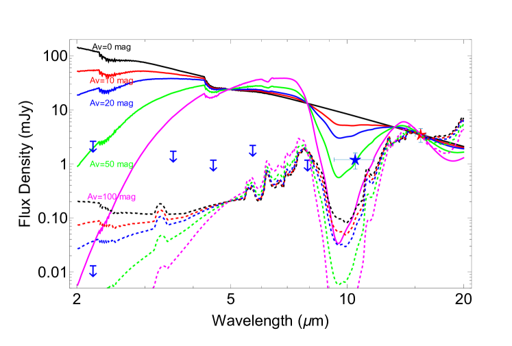
Figure 4: Limits from archival imaging at ’s position. The solid, color-coded lines show a photospheric model for an M0III star ( K) reddened by increasing levels of extinction, all normalized to 3.5 mJy at 15.5 m (red star). The blue star denotes the flux density of the object denoted detected by the VLT/NEAR experiment (Wagner et al., 2021). The dashed lines show the spectral energy distribution of a typical star-burst galaxy or ULIRG (Arp 220) similarly reddened. Upper limits at the position of come from observations at earlier epochs with Spitzer/IRAC (3–8 m), 2MASS, and NACO (Kervella et al., 2016). 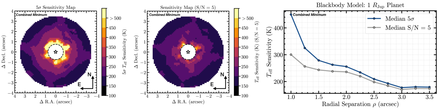
Figure 5: Left: two-dimensional 5 planet effective blackbody temperature sensitivity map, combined across all epochs by selecting the best sensitivity (“combined minimum”, see Paper II), in sky coordinates (North up, East left). The central region ( 075, or 1.5 FWHM, radial separations) is masked (poor detectability). A discrete colormap is chosen to highlight the different sensitivity zones across the image. Center: same as the left panel for a S/N = 5 detection threshold. Right: 5 and S/N = 5 median planet effective blackbody temperature curves combined across all epochs. -
•
We eliminate the possibility that is a foreground Solar System object in a number of ways. An inner main belt asteroid (MBA) at 2.2 AU with a typical temperature of 200 K would have to have a diameter of 2 km to emit 3 mJy at 15.5 m. Such objects are extremely rare, brighter than 3 mJy at 12 m in a 5′5′ field at Cen A’s ecliptic latitude of (Brooke, 2003). Furthermore, the completeness for such large MBAs is over 90% and the Minor Planet Catalog shows no known objects at the position of Cen A at the August epoch444https://minorplanetcenter.net/cgi-bin/checkmp.cgi. Finally, as described in Paper II, there is no angular motion seen between the beginning and the end of 2.5 hour MIRI observation compared to the expected 10 arcsec/hr motion for an MBA at the solar elongation of our observations, (Brooke, 2003).
Based on all of the above considerations, we pursue the hypothesis that is a planet physically associated with and in orbit around Cen A, as opposed to an artifact or an astrophysical contaminant, and investigate its properties. Given that is only detected in a single roll observation in August 2024, we emphasize that it is, at the moment, a planet candidate. Additional sightings of are required with JWST, or other upcoming facilities, to confirm what would be “ Cen Ab”.
3.3 Planet Detection Limits with JWST/MIRI
We assess our sensitivity to planets around Cen A across all three epochs of MIRI F1550C observations. Paper II (Sanghi & Beichman et al., 2025) presented the calculation of 2D flux/contrast sensitivity maps. Here, we use the “combined minimum” map from Paper II, which corresponds to the 2D sensitivity map with the best flux sensitivity across all three epochs at each location where the PSF injection-recovery test was performed. We convert the 5 and S/N = 5 flux sensitivities (see Paper II) to effective temperatures () assuming a blackbody model and a typical planet radius of 1 (for smaller planets, the minimum detectable planet increases). The results are shown in Figure 5. The MIRI F1550C observations are sensitive to 250 K (1 ) planets between 1″–2″ for a S/N = 5 detection threshold. Planets colder than 200 K can be detected at wider separations ( 25). We note here that more realistic planet atmospheric models may have a higher brightness temperature (and thus flux) in the F1550C bandpass relative to the effective blackbody temperature assumed here (see §5.2, for example). This would improve the detectability of colder planets at smaller separations than presented here.
3.4 Limits on Extended Emission around Cen A
Beichman et al. (2020) predicted that JWST’s ability to resolve the habitable zone around Cen A would result in unprecedented sensitivity to warm dust—the analog of the thermal emission from dust generated by collisions the asteroid belt in our solar system. We show below that the current observations have not only met but exceeded those expectations with limits as low as a few times the solar system brightness levels at 15.5 m.
3.4.1 Exozodi Model Description
As described in Paper II, we injected a number exozodiacal cloud models into the processed Cen datacubes to set limits on extended “exozodiacal” emission around Cen A. In the case of Cen A, stable orbits—and thus significant dust buildup—are limited to within the stable zone, approximately 3 au from the star. The Solar System zodiacal cloud is therefore a poor proxy for a potential exozodi around Cen A. For a more realistic representation, we consider the scenario of an asteroid belt analogue (ABA) located between 2–3 au, where dust is produced in collisions, which is then transported inward under Poynting-Robertson (PR) drag. This scenario is captured by the semi-analytical model of Rigley & Wyatt (2020), which combines approaches to determine (1) the size distribution arising in a planetesimal belt under collisions and PR drag loss (Wyatt et al., 2011), and (2) how it evolves interior to the belt under further collisional and drag-induced evolution (Wyatt, 2005). The resulting optical depth distribution (across grain sizes and disk radii) is then combined with the particles’ thermal emission properties, determined using Mie theory, to compute the disk’s surface brightness distribution.
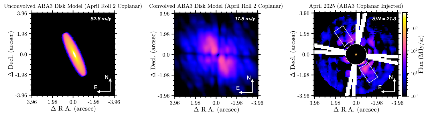
Following the approach of Sommer et al. (2025), we generate astrophysical scenes of the inclined, edge-on disks from the respective surface brightness profiles, and convolve them with the spatially varying PSF of the F1550C coronagraphic filter (modeled using STPSF, Perrin et al., 2014), before injecting them into the MIRI datacubes. An example of an exozodi scene, before and after PSF convolution, alongside a PSF subtracted image obtained after model injection, is shown in Figure 6. Note that all exozodiacal disks considered here are assumed to be coplanar with the Cen AB plane, which is a reasonable assumption for potential circumstellar debris disks in binaries (see Section 6.2.1), although the invariable plane about which the orbit precesses could also be affected by the gravity of massive planets in the system.
| Model | () | () | (Gyr) | (mJy) | S/N | |||||||
|---|---|---|---|---|---|---|---|---|---|---|---|---|
| ABA 1 | 20 | 28 | 0.88 | 596 | 69 | 1.04 | 0.29 | 0.76 | 94 | 58 | 84 | 78.7 |
| ABA 2 | 4 | 5.6 | 4.40 | 156 | 18 | 0.27 | 0.07 | 0.17 | 27 | 17 | 29 | 52.6 |
| ABA 3 | 2 | 2.8 | 8.80 | 53 | 6.1 | 0.09 | 0.04 | 0.09 | 8.3 | 5.1 | 8.4 | 21.3 |
| ABA 4 | 1.2 | 1.7 | 14.5 | 20 | 2.3 | 0.03 | 0.02 | 0.06 | 3.0 | 1.8 | 3.0 | 5.8 |
| 1-zodi | 8.8 | 1.0 | 0.02 | 0.02 | 0.06 | 1.5 | .94 | 1.0 | 0.7 |
Note. — Exozodi models used for injection and derived quantities. Columns: , ABA model dust mass parameter (belt mass up to cm grain size); , ABA model belt mass up to largest planetesimal () in units of Solar System main asteroid belts (); , collisional lifetime of largest planetesimal; , total disk flux at 15.5 m; , fractional disk flux at 15.5 m; , photometric significance (phot. sig.) for MIPS24; , phot. sig. for PACS70; , phot. sig. for PACS100 (all uncertainties from Wiegert et al., 2014); , fractional disk luminosity; , zodi level by fractional luminosity; , zodi level by Earth Equivalent Insolation Distance (EEID) surface density; and S/N ratios of injection recovery tests with the April 2025 dataset for the case of binary-coplanar disks.
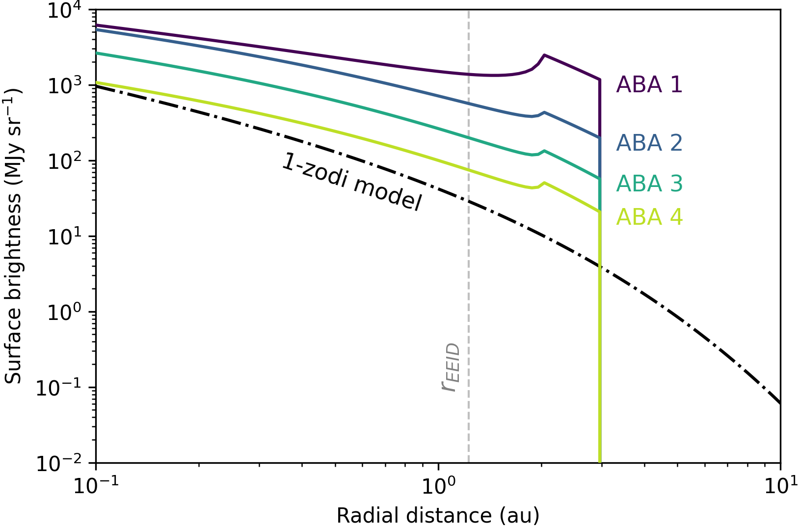
For the model parameters, we further assume a belt opening angle of 5∘, a size-independent catastrophic disruption threshold of erg g-1 (representing the grains’ collisional strength), as well as a grain composition of 1/3 amorphous silicates and 2/3 organic refractories by volume, which determines their Mie-theory-derived optical properties. Four models of different belt dust masses, ABA 1–4, are considered, for which derived quantities are summarized in Table 3. The resulting surface brightness profiles of the different models are compared in Figure 7. Here, the ABA-1 model differs from the other models in having a sharper decline of surface brightness at the inner belt edge. This is because, at that mass, even small dust is effectively ground down to blowout sizes before it can migrate inward past the belt. As a result, further increases in belt mass only enhance the local brightness within the belt, while the interior regions reach saturation (Wyatt, 2005).
To give an indication of the plausibility of the ABA models, we also conduct a simplified analysis of total belt mass and collisional lifetimes within the belt, assuming a canonical collisional cascade with a size distribution following a power-law slope of (Dohnanyi, 1969) extending up to a maximum planetesimal size of . Comparing the collisional lifetime of the largest planetesimal to the system age of Cen ( 5 Gyr) shows that the ABA-1 model is likely not viable, since even with planetesimals as large as , collisions would have inevitably eroded the planetesimal belt to below the ABA-1 level over the system age. In contrast, ABA-2 is marginally consistent with the anticipated level of erosion, while ABA-3 and ABA-4 are more readily compatible with the system’s age, only requiring planetesimal masses of a few times that of the Solar System’s main asteroid belt. Nevertheless, we retain the ABA-1 model in this analysis for comparison purposes.
For reference, we also include an exozodi model that is similar to the Solar System zodi, even though its radial extent is non-physical around Cen A. This fiducial “1-zodi” model is derived from the Kelsall et al. (1998) geometrical model for the Solar System’s dust cloud, which was fitted to infrared zodiacal light observations by COBE/DIRBE. Here we use the radial surface density distribution approximation derived by Kennedy et al. (2015) for the Kelsall et al. (1998) model. Using the emissivities fitted by Kelsall et al. (1998), we calculate the disk’s corresponding surface brightness distribution at 15.5 m, which is also shown in Figure 7. We then use the same image synthesis pipeline as with our ABA exozodi models, the result of which closely matches the outcome of applying the zodipic model—an IDL implementation of the Kelsall et al. (1998) model (Kuchner, 2012)—around Cen A (see Beichman et al., 2020), and likewise inject this 1-zodi model into the MIRI datacubes.
While our ABA exozodi models are not strictly comparable to the Solar System’s zodiacal cloud in terms of geometry, it is still useful to define a “zodi level” that quantifies the dust content of the disks relative to the Solar System. Two wavelength-independent metrics for this are the total disk luminosity and the surface density within the habitable zone (HZ). The luminosity-based zodi level is defined as the ratio of the exozodi’s fractional luminosity to that of the Solar System’s zodiacal cloud:
| (1) |
while the surface-density-based zodi level is given by the ratio of the disk surface density at the Earth-equivalent insolation distance (EEID), —approximately for Cen A—to that of the Solar System at ():
| (2) |
with (Kennedy et al., 2015). As discussed by Kennedy et al. (2015), serves as a proxy for the exozodi’s surface brightness in the HZ and is therefore useful for assessing its impact on direct imaging of Earth-like planets. Both definitions of the zodi level are provided in Table 3 for our set of models.
3.4.2 Comparison with Previous Exozodi Searches
The results of the injection-recovery analysis of our various exozodi models, presented in Paper II (Sanghi & Beichman et al., 2025), are summarized by the corresponding S/N values in Table 3. In summary, these observations are sensitive to emission from an exozodiacal cloud that is coplanar with the binary orbit at a level of or . This represents an unprecedented sensitivity compared with previous observations and is facilitated by the system’s proximity and the model disks’ near-edge-on orientation, which our recovery method is tailored to (see Sanghi & Beichman et al., 2025).
It is first worth acknowledging that previous photometric searches have not detected significant excess dust emission at any wavelength (Wiegert et al., 2014; Yelverton et al., 2019). While Wiegert et al. (2014) suggest a Spitzer/MIPS excess at 24 m at , even our brightest model disk, ABA-1, yields an excess at 24 m of only around (see Table 3). Since the ABA-1 model would have easily been detected by our observations, we can confidently rule out the presence of a static (inclined) exozodi to have caused the reported feature. Excesses of our model disks in the far-IR for Herschel PACS70 and PACS100 observations are of even lower significance, consistent with previous non-detections. This means that any circumstellar disk would have to be even more massive than ABA-1 to have shown up in previous mid- and far-IR photometric observations, indicating that our observations which could detect ABA-3 are at least 10 times more sensitive in terms of the belt’s dust mass.
This improvement in sensitivity arises because photometric observations do not provide the most stringent limits on the presence of dust, due to calibration uncertainties that limit detectable excesses to typically more the 10% of the stellar flux (Beichman et al., 2005), but with sensitivity approaching 2% in recent studies with JWST (Farihi et al., 2025). By that metric it is clear that our resolved imaging approach is able to improve on that limit by about two orders of magnitude, since we were able to successfully suppress the stellar emission to recover the signal of the ABA-3 model which has an excess of % at m (see Table 3). In principle, lower dust levels than simple photometry can be achieved using nulling interferometry to suppress the stellar emission. The largest and deepest survey of this kind was the HOSTS survey which used the LBT interferometer (LBTI) to search for exozodi emission in the habitable zone at m. While Cen A was not included in that survey, due to its Southern hemisphere location and its binarity, the survey results show that the best sensitivities achieved for (single) solar-type stars reached as low as % on the null depth, which corresponds to limit of % for the total flux required for a detection (Ertel et al., 2018, 2020). That is, our imaging observations achieved a limit at least five times lower than is achievable with nulling interferometry. A similar conclusion is reached by comparing the 5–8 zodi levels of the ABA-3 model (see Table 3) with the best reported zodi limits from the HOSTS survey of 70 zodis. This is similar to the sensitivity level of previous mid-infrared coronagraphic imaging of Cen A with VLT/VISIR, since Wagner et al. (2021) reported a resolved source () that could be fitted with a 60 zodi () exozodi model. Such a disk would be in between our ABA-1 and ABA-2 models, and thus would have been easily detected by our observations. We can thus rule out that belongs to a static clump of exozodi material at this level. The comparisons with previous observations demonstrate the dramatic improvement in sensitivity achieved by the JWST measurements.
| Sightings Used | Orbit Type | aaInclination relative to the Cen AB orbital plane (, from Akeson et al., 2021). | bbInclination relative to the plane of the sky. Bimodal distributions (about ) are presented as two sets of values. | ccFlux-averaged mean planet temperature for (see §5.1) | ||
|---|---|---|---|---|---|---|
| (au) | (∘) | (∘) | (K) | |||
| , , & NDddND denotes that orbits were checked for consistency with non-detections in the February and April 2025 epochs. | Prograde, au | or | ||||
| No RV Constraint | ||||||
| , , & ND | Prograde, au | or | ||||
| m/s | ||||||
| , , & ND | Prograde, au | |||||
| m/s | ||||||
| , , & ND | Prograde, au | |||||
| No RV Constraint | ||||||
| , , & ND | Prograde, au | |||||
| m/s | ||||||
| , , & ND | Prograde, au | |||||
| m/s | ||||||
| , , & ND | Retrograde, au | or | ||||
| No RV Constraint | ||||||
| , , & ND | Retrograde, au | or | ||||
| m/s | ||||||
| , , & ND | Retrograde, au | |||||
| m/s | ||||||
| , , & ND | Retrograde, au | |||||
| No RV Constraint | ||||||
| , , & ND | Retrograde, au | |||||
| m/s | ||||||
| , , & ND | Retrograde, au | |||||
| m/s |
Note. — Parameters are reported as mean standard deviation. assumes a planet mass of 100 .
4 Orbital Modeling of +
With only a single JWST/MIRI sighting (and non-detections at two other epochs), it is challenging to uniquely constrain the orbit of . To make progress, we consider the family of orbits that (a) fit the relative astrometry of and the VLT/NEAR 11.25 m candidate (Wagner et al., 2021), which we treat as an earlier detection of the object ; (b) are dynamically stable in the presence of Cen B; and (c) are consistent with the non-detection of in the February and April 2025 observation epochs. Additionally, we consider the consistency of the candidate’s orbits with existing RV upper limits.
4.1 Selection of Stable Orbits
First, we randomly generate orbits matching the astrometry of and (Table 2) using the Orbits For The Impatient (OFTI) algorithm via the orbitize! package (Blunt et al., 2017, 2020). We apply the default priors in the orbitize! code to the candidate planet’s orbital elements and use a Gaussian prior for Cen A’s mass and parallax (, mas, from Akeson et al., 2021). Next, we evaluate the stability of the accepted orbits using the -body simulation software Rebound (Rein and Liu, 2012) over million year timescales using the WHFAST integrator (Rein et al., 2019). A given simulation is deemed unstable for very high planetary eccentricity or large planetary distances from the host star . Previous studies showed that orbits that meet either criterion are very likely to be unstable on billion-year timescales (Quarles & Lissauer, 2016, 2018), where more than of orbits stable on a million-year timescale were also stable for billion-year timescales. We find that 30% of the orbits from the initial orbitize! sample are dynamically stable.
4.2 Incorporating Constraints From Non-Detections
We investigate which of the above stable orbits are consistent with non-detections in the February and April 2025 observation epochs using the 2D sensitivity maps generated for both epochs in Paper II (Sanghi & Beichman et al., 2025). Specifically, we use the S/N = 5 sensitivity map (rather than the 5 significance sensitivity map) to be stricter in eliminating orbits where would have been marginally recovered in our follow-up observations. The sensitivity maps provide the minimum point source flux detectable at a S/N = 5 at different sky coordinates around Cen A. For each of the stable orbits above, we predict the sky position of the candidate planet in the February and April 2025 observations, and check the corresponding location in the sensitivity map to evaluate whether it would have been detected (for a flux of 3.5 mJy). Orbits where the candidate would have been recovered in either of the two epochs are eliminated. We find that 52% of the stable orbits that fit the astrometry are also consistent with non-detections in both February and April 2025 (Figure 8). There is, thus, an a priori significant chance that, if real, the planet candidate could have been missed in both follow-up observation epochs.
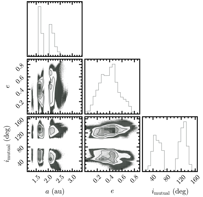
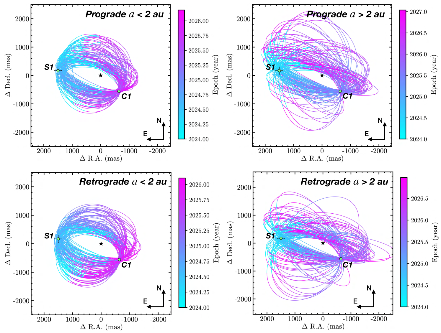
The posteriors for the three key orbital elements (semi-major axis , eccentricity , and mutual inclination with respect to the Cen AB binary orbit555The mutual inclination is calculated using Equation 19 in Xuan & Wyatt (2020) and using the orbital parameters for Cen AB in Akeson et al. (2021).) of the stable orbits consistent with the non-detections (Figure 9) show that there are four families of orbits666We do not consider the small fraction (0.2% of the total number) of au orbits in Figure 9 as they do not agree with ’s relative astrometry within 1 uncertainties.. They correspond to the number of orbital periods that have elapsed between the VLT/NEAR observations in June 2019 and the JWST detection in August 2024 (either 1.5 or 2.5 periods, for 1.6 au and 2.1 au, respectively) and orbits in either the prograde () or retrograde () direction (Figure 10). In addition to being significantly inclined, the planet candidate is in a moderately eccentric () orbit. A summary of the mean orbital parameters for each family (no RV constraint case) is provided in Table 4. Note that all orbits presented are dynamically stable as evaluated previously (§4.1).
4.3 Consistency with RV Limits
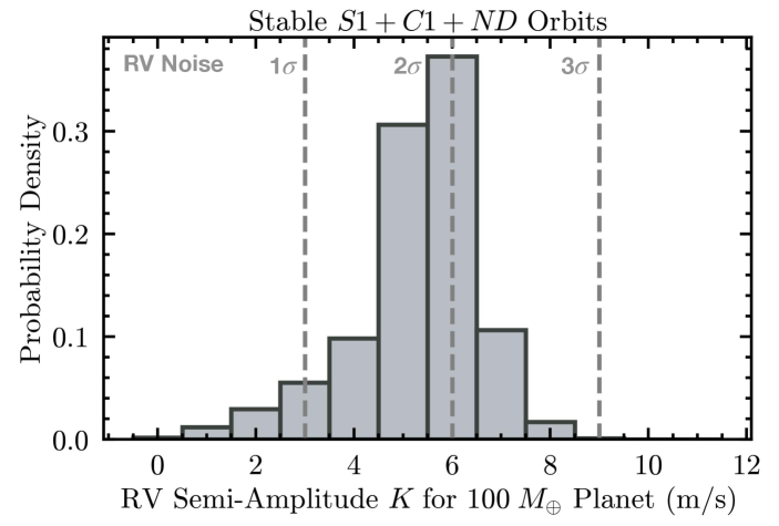
To the family of stable orbits consistent with non-detections, we can add a constraint of m s-1 (; Butler et al., 2004; Zhao et al., 2018) on the radial velocity of Cen A, which is also observed in the HARPS RV residuals (Kervella et al., in preparation). This systematic noise floor constrains the minimum mass () of any planet around Cen A to be (2) or (3) within au. Among the dynamically stable orbits consistent with the non-detections, assuming , we find that 4% of these orbits result in 3 m/s, 50% result in 6 m/s, and 99.8% of all orbits result in 9 m/s (Figure 11, the maximum is m/s). Table 4 presents orbital parameters for each case. The semi-major axis and eccentricity remain largely unchanged after applying the RV constraints; however, the mutual and sky inclinations vary as the RV constraint becomes stricter (smaller reflex motion). In summary, the astrometric positions of can be fit by dynamically stable orbits consistent with both the non-detections in follow-up observations and existing RV limits. All dynamically stable orbits consistent with non-detections can be retrieved from10.5281/zenodo.16280658 (catalog 10.5281/zenodo.16280658).
5 Photometric Modeling of +
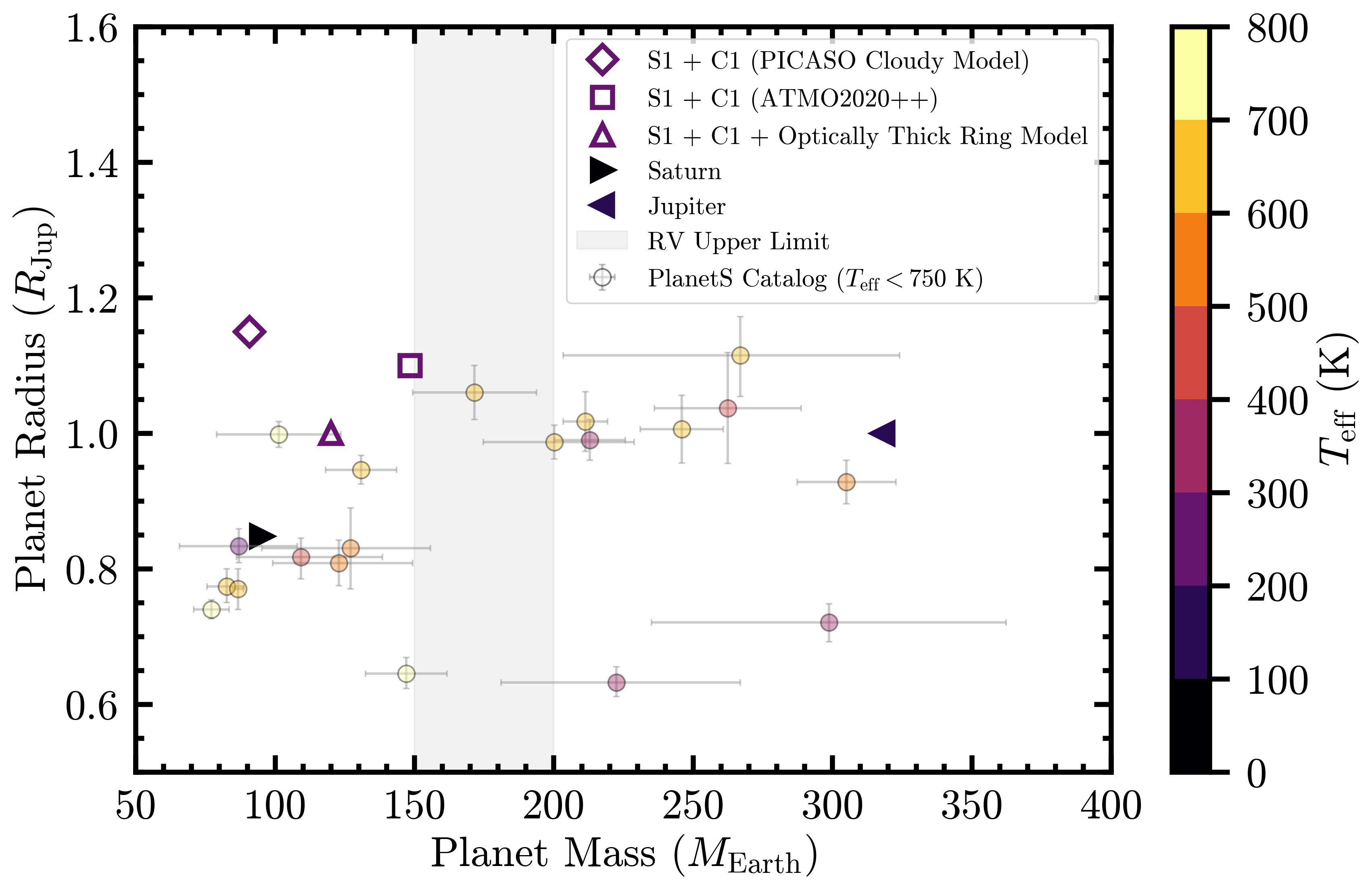
In this section, we consider the available photometric data points for the Cen A planet candidate (JWST/MIRI 15.5 m and possibly, VLT/NEAR 11.25 m) to investigate its bulk physical properties. While the photometric data are sparse at the moment, there are some physical constraints that can be applied to aid modeling efforts. First, the effective temperature of the planet candidate is expected to be set by heating from Cen A. Second, the radius of a mature (5 Gyr) gas giant planet cannot significantly exceed 1–1.2 (allowing for some variations if the planet is rapidly rotating and viewed pole-on, for example) unless it is located in a very tight “Hot Jupiter” orbit, which is not the case as seen in the previous section on orbital modeling. Finally, the mass of the planet must be consistent with the limits set by the radial velocity measurements (Zhao et al., 2018). Subject to these constraints, we examine a range of plausible atmospheric models as well as thermal emission from a Saturn-like particle ring to explain the photometric data.
5.1 Equilibrium Temperature
We use the orbital information to infer the range of plausible effective temperatures for the planet candidate, heated by Cen A. The equilibrium temperature for a planet on an eccentric orbit depends on the instantaneous stellar input, the planet’s thermal inertia, and radiative timescale. For a gas giant planet, any variations of temperature through the orbit are damped by the thermal inertia of the dense H/He atmosphere (Quirrenbach, 2022). In such a scenario, the correction to the equilibrium temperature to account for changes in the insolation averaged over an eccentric orbit are small, only a few percent, for eccentricities up to 0.5 (Johnson & McClure, 1976; Quirrenbach, 2022). The flux-averaged temperature of a body heated by and orbiting Cen A in an eccentric orbit, , at a distance is given by
| (3) |
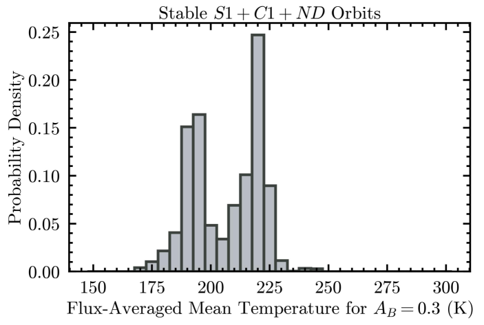
where K (Zhao et al., 2018), (Akeson et al., 2021), is the Bond albedo, and full heat re-distribution () is assumed. Adopting = 0.3 (intermediate between the values for most Hot Jupiters and those of the Solar System gas giants), we compute for all stable orbits consistent with the non-detections (§4) and find a bimodal distribution with peaks at 195 K and 220 K (Figure 12). The lower temperatures correspond to orbits in the au families and the higher temperatures correspond to orbits in the au families (Table 4).
The contributions of additional sources of heat for the planet candidate’s temperature are negligible compared to stellar insolation. (1) Residual heat of formation: Cen A is 5 Gyr old. For a similar internal radiation flux () as Jupiter or Saturn, 110 K (Li et al, 2018), the increase in temperature is negligible, due to and the planet candidate’s higher expected . (2) Radiation from Cen B: Cen B is less luminous than Cen A by a factor of 3 (Akeson et al., 2021) and at the time of JWST observations was 20 au away from Cen A. Thus, its contribution to heating is negligible. (3) Tidal heating: the candidate is in an eccentric orbit. However, (Peale & Cassen, 1978) is negligible for au. (4) Heating from radioactivity: this is negligible for Neptune, which is both much colder than and likely has a larger fraction of radioactive isotopes.
5.2 Planet Atmospheric Models
The goal in this section is to obtain first estimates of the planet candidate’s fundamental parameters (, radius, and mass) using atmospheric model grids available in literature for cold planets and brown dwarfs. Given the numerous atmospheric parameter degeneracies involved in fitting two photometric data points, particularly in the observationally unexplored low-mass ( 200 ), low temperature ( 300 K) planetary regime (see for example, Crotts et al., 2025), we aim only to provide example scenarios that can explain the observed flux measurements. Detailed atmospheric modeling is appropriate for future studies when additional photometry and/or spectroscopy is available (see §6.3).
We jointly fit the F1550C JWST/MIRI flux and the 11.25 m VLT/NEAR flux (Table 2), assuming they are related (as indicated by the orbit fits in the previous section). The fitting procedure synthesizes model photometry in the F1550C bandpass (15.15–15.85 m, using the transmission curve from the SVO filter profile service777http://svo2.cab.inta-csic.es/theory/fps/) and the VLT/NEAR bandpass (10–12.5 m, constant transmission assumed), and finds the minimum radius ( 1.2 ) that yields a model flux consistent with the measured photometry within 1. The effective temperature of the planet is set to 225 K for the atmospheric models fit below, matching that expected for au orbits (Table 4)888We were unable to fit the photometry with 200 K models for planet radii 1.2 .. We also restrict the surface gravity (log , in CGS units) of the models to 2.5–3.0 dex, chosen to yield a planet mass 150–200 to be consistent with radial velocity limits ( , 3; inclined orbits can raise the limit on the true planet mass).
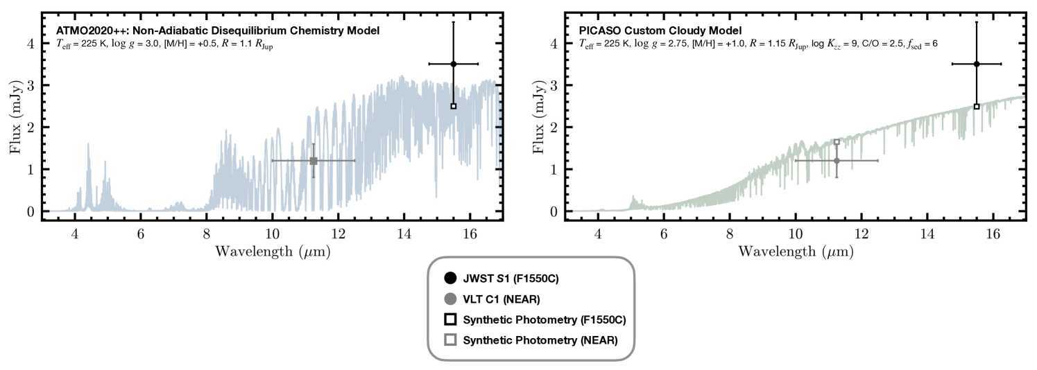
ATMO2020++ (Leggett et al., 2021; Meisner et al., 2023): Using the ATMO2020 models with strong vertical mixing as a starting point, ATMO2020++ modifies the adiabatic ideal gas index (and thus atmospheric temperature gradient) to account for the effect of processes responsible for producing a non-adiabatic cooling curve in giant planet and brown dwarf atmospheres. These processes include complex atmospheric dynamics (e.g., zones, spots, waves) due to rapid rotation, compositional changes due to condensation, upper atmosphere heating by cloud decks or breaking gravity waves, etc. Recent modeling with JWST data has shown that this grid provides an improved fit to Y dwarf spectra compared to the standard-adiabat models (Leggett & Tremblin, 2023, 2024; Luhman et al., 2024). The default ATMO2020++ grid only extends to K, so we generated custom models for K, log dex, and [M/H] . We find that the K, log dex, and [M/H] model agrees with the photometry for a radius of 1.1 (Figure 13). For the above parameters, the planet candidate would have a mass 150 .
Sonora and PICASO models: The Sonora Flame Skimmer models (Mang et al., in prep) extend the cloud-free Sonora Elf Owl grid (Mukherjee et al., 2024; Wogan et al., 2025) to colder effective temperatures, lower surface gravities, and a broader range of metallicities. These models incorporate rainout chemistry for H2O, CH4, and NH3—even in cloud-free atmospheres—similar to the treatment in Sonora Bobcat. They also address the underestimation of CO2 found in the Sonora Elf Owl models (Mukherjee et al., 2024), which has since been revised in Wogan et al. (2025). In addition, we generated a custom grid of cloudy models using PICASO (Batalha et al., 2019; Mukherjee et al., 2023). This grid spans effective temperatures of and 225 K, surface gravities of log = 2.75 and 3.0 dex (cgs), eddy diffusion coefficients and cm2 s-1, metallicities of [M/H] = +0.5 and +1.0, and a C/O ratio of 2.5 (relative to solar). Cloudy models have = [4, 6, 8], with H2O as the only condensing species. We find that the K, log dex, [M/H] , log , C/O = 2.5, model agrees with the photometry for a radius of 1.15 (Figure 13). For the above parameters, the planet would have a mass 90 .
Additional models applicable to cool giant planets: We also experimented with fitting the photometry using the Sonora Bobcat cloudless, chemical equilibrium model grid (Marley et al., 2021), the ATMO2020 solar metallicity, disequilibrium chemistry model grid (Phillips et al., 2020), the patchy water cloud models of Morley et al. (2014), and a new grid of self-consistent models by Lacy & Burrows (2023) that incorporate both the effects of water clouds and disequilibrium chemistry. However, we did not find suitable solutions with these grids, as they all required a K to fit the photometry for a radius .
5.3 Planet Ring System Models
The previous section presented example planet models which can reproduce the brightness of , but required planet radii (driven by the observed F1550C brightness), more commonly observed for hotter planets, but plausible if a rapidly rotating planet is viewed closer to pole-on (the observed surface area can be higher). Alternate explanations for the F1550C brightness include (1) a knot of exozodiacal emission; or (2) a smaller planet with a circumplanetary ring. Given the lack of exozodi detection reported in §3.4, we do not consider the exozodi knot interpretation further, except to note that this would require the knot to dominate the exozodi emission, and for the knot to orbit the star with similar constraints to those reported for the planet scenario (§4) and to have only been detected at one epoch of our observations.
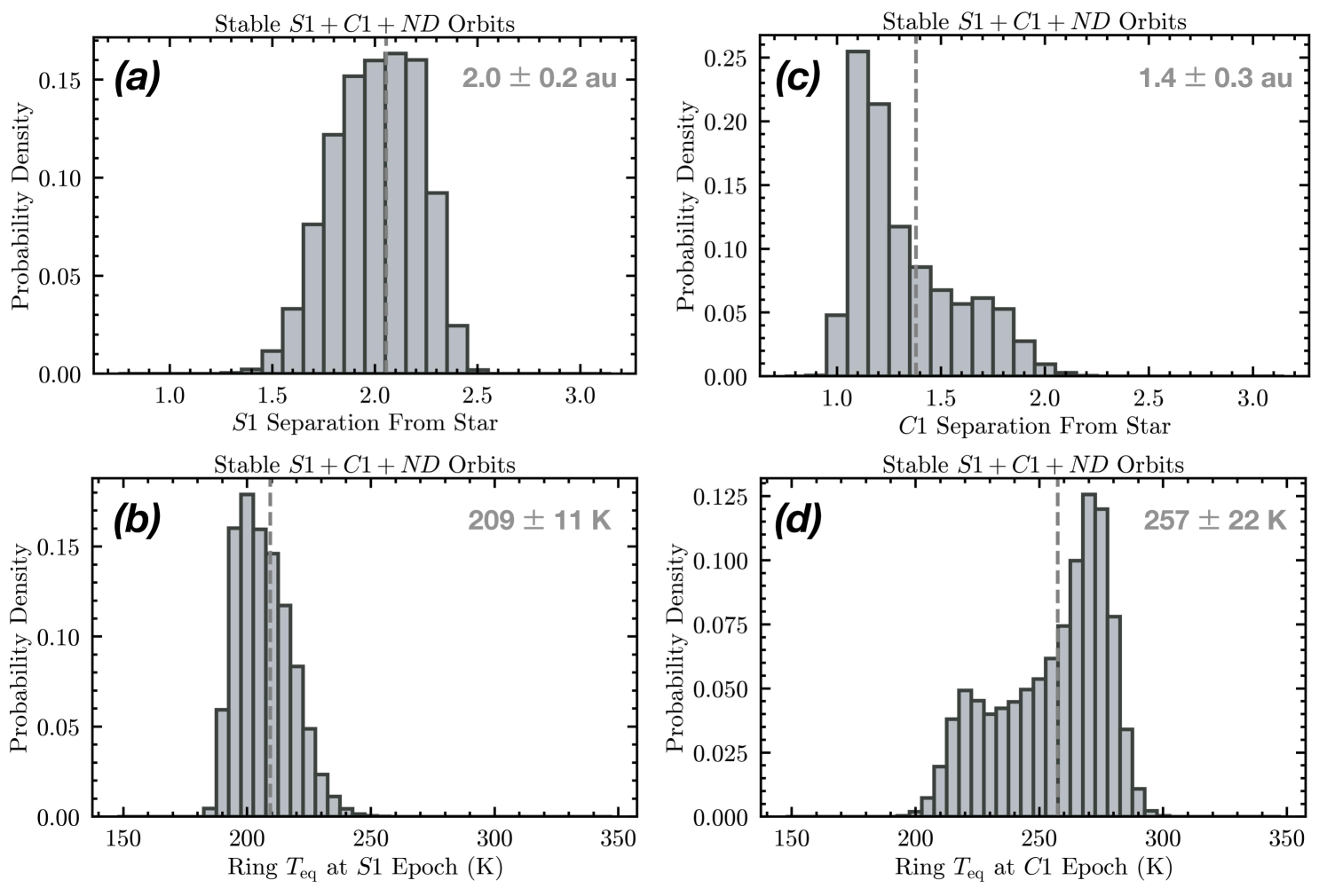
For an interpretation of the emission as circumplanetary material, a straight-forward model is to consider an optically thick ring. A ring is not expected to have significant thermal inertia (as opposed to a gas giant planet, as discussed in §5.1). Thus, the ring temperature at the and detection epochs will be the instantaneous equilibrium temperature calculated for the true planet-star separation at those epochs. For each stable orbit consistent with the non-detections in the prograde au family, we calculate the planet-star separation and the corresponding equilibrium temperature, assuming (similar to asteroids) and (Figure 14). Orbits with au are favored as they yield a higher planet , which is required to better fit the F1550C brightness (the prograde and retrograde scenarios yield similar separation distributions and mean values). We find that an optically thick circumplanetary ring would be hotter at the epoch ( K) than at the epoch ( K).
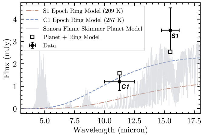
We modeled the observed photometry using various 225 K planet atmospheric models (grids discussed in §5.2) combined with a constant surface area (free parameter) blackbody ring with a temperature of 257 K for the VLT/NEAR 10–12.5 m flux and a temperature of K for the F1550C flux. The photometry agrees, within 1 uncertainties, with a Sonora Flame Skimmer clear, equilibrium, K, log = 3.0 dex, [M/H] = +1.0, and C/O = 1.5 model for a planet radius of 1 (corresponding to ), together with a ring that has a cross-sectional area equivalent to a face-on disk of radius 64,000 km or 0.9 (Figure 15). This is half the cross-sectional area of Saturn’s rings, which extend to 140,000 km (plus a more tenuous, more distant distribution). Planetary rings lie in their planet’s Roche zone from 1.4–2.5 , so this explanation seems plausible.
We stress that the ring model discussed above is highly simplified. Geometrical effects make it challenging to develop a fully comprehensive and accurate optically thick ring model. The inclination of the ring with respect to the star affects the ring’s temperature. The inclination of the ring to our line-of-sight together with shadowing of the ring by the planet affects the inferred size and visible emitting area. Additionally, a ring could both shade the planet from starlight, reducing planet temperature, and block planet light towards the observer. In the absence of strong constraints on the planet candidate’s orbit and with only two photometric points, the problem is highly unconstrained. Overall, the key takeaway of the analysis presented above is that a circumplanetary ring around the planet candidate is a plausible hypothesis to explain the higher F1550C brightness for a smaller planet than inferred just using atmospheric models. A summary of the inferred mass and radius of the candidate from both atmospheric and ring models, as compared with the cold transiting planet population, is presented in Figure 16.
For completeness, we consider an alternative model for circumplanetary material, where the cross-sectional area derived above comes from an optically thin dust distribution, such as one that might arise from the grinding down of a cloud of irregular satellites orbiting the planet (Kennedy et al., 2011). Such a cloud could extend out to roughly half the Hill radius of the planet ( au radius for a low eccentricity, 100 planet at 2 au), which would correspond to a distribution with optical depth . Small grains with realistic optical properties, in models in which the dust is optically thin, are heated above blackbody temperature. This increases the flux in the VLT/NEAR bandpass and makes it more challenging to simultaneously fit the and photometry, specifically because the ring is expected to have a higher temperature at the detection epoch than the detection epoch from planet-star separation calculations (Figure 14). This would require the dust distribution to be truncated to avoid the presence of m-sized dust. This is in addition to the challenge of retaining the irregular satellites given their expected collisional erosion.
6 Discussion
We start by investigating possible mechanisms to explain the high eccentricity and inclination orbits inferred for the candidate in a close binary system like Cen AB. We then briefly discuss the prospects for other planets or an exozodiacal disk around Cen A in the presence of the candidate, and end with a discussion of implications of a gas giant in Cen AB system in relation to theories of planet formation in binary systems.
6.1 Planetary Companions
6.1.1 Secular Dynamics of S1 + C1 Planet Candidate
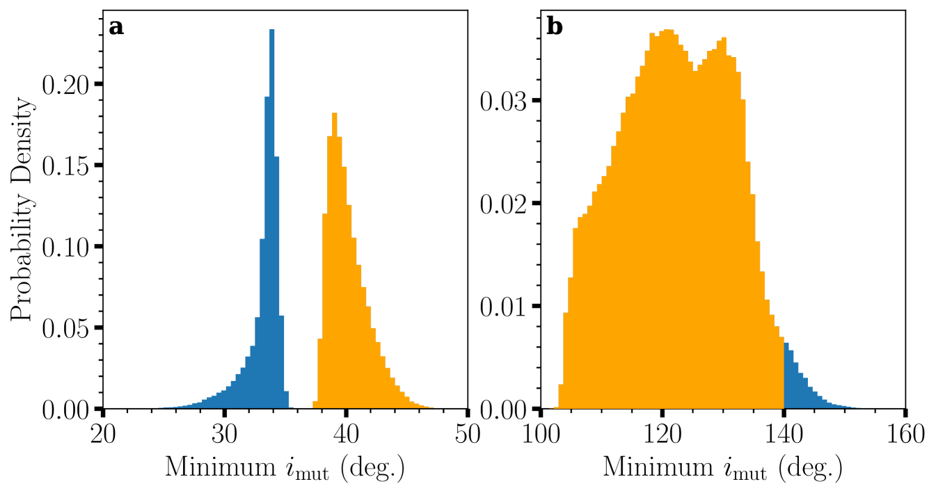
Table 4 reveals that the best fitting orbits for consistent with the non-detections are significantly inclined with respect to the Cen AB binary orbital plane and eccentric, which naturally leads one to suspect that the planet candidate might undergo von Zeipel-Kozai-Lidov (vZKL) oscillations. (von Zeipel, 1910; Kozai, 1962; Lidov, 1962; Ito & Ohtsuka, 2020). In the test particle approximation (Naoz, 2016) for vZKL oscillations, the less massive body () will have a minimum mutual inclination relative to the more massive binary, which is approximately for prograde and for retrograde orbits. Figure 17 shows the probability density of minimum inclination attained during our N-body stability simulations selecting on the stable orbits that fit and are consistent with non-detections. The minimum mutual inclination shows that a majority of orbits undergo vZKL oscillations, likely to be large amplitude, in the test particle approximation and consistent with the candidate’s present configuration.
6.1.2 Prospects For Other Planets Orbiting Cen A
The Hill Radius, , gives a measure of the relative gravitational influence of two bodies on a third and can be used to identify regions in semi-major axis for the stability of a third body. We use this to assess the possibility that another planet might exist in the Habitable Zone (HZ) of Cen A given the presence of a planet with the properties of + . The Hill Radius, is given by:
| (4) |
Given the best-fit semi-major axis, , and eccentricity, , for each of the potential orbital families (Table 4), using the host star mass M, and assuming a candidate planet mass M, the Hill Radius for semi-major axis, =1.62–2.16 au and , ranges from 0.044–0.060 au. Quarles, Lissauer & Kaib (2018) argue that for stability in a coplanar system, a buffer zone of is required to establish stable orbits in a two planet system. Thus, it is unlikely for there to be any other planets between and , i.e., . Thus, assuming the candidate is real, there are probably no other planets within or exterior to Cen A’s HZ.
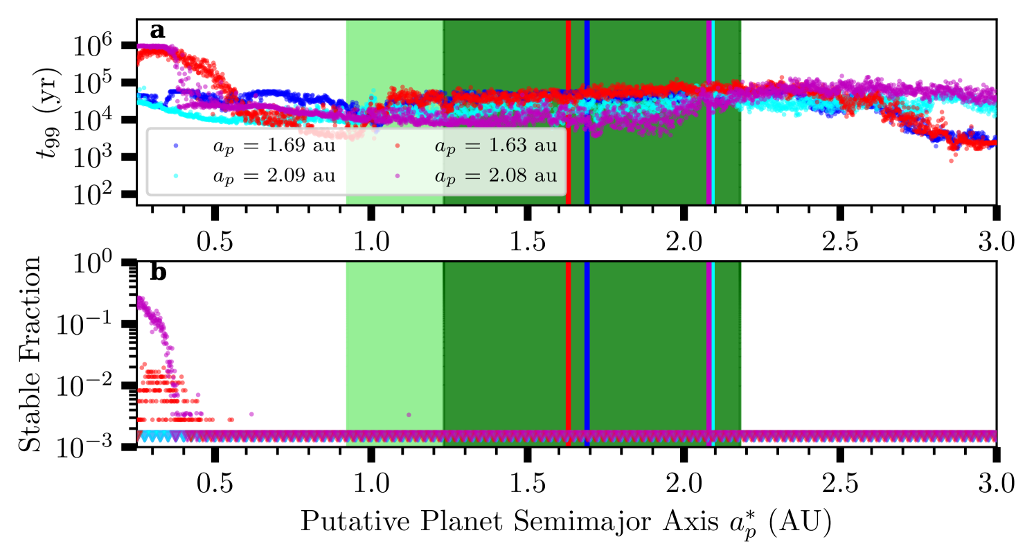
These arguments are bolstered with numerical simulations which show, with the parameters of , there are no stable orbits exterior to au (Figure 18). These simulations use the N-body simulation package Rebound with the IAS15 integrator, where the massive bodies (binary + ) begin with the mean orbital parameters from the cases in Table 4 for and stellar parameters from Akeson et al. (2021). The putative second planet begins as a test particle on a slightly eccentric orbit that is apsidally aligned and coplanar with , where we vary the putative second planet semi-major axis from with steps of and initialize the mean anomaly of the body from in steps of . The simulations are evolved for 1 Myr, where an individual simulation is stopped depending on the state of the test planet, which can either be ejected (distance of the test planet exceeding ), have high eccentricity , or collide with either or the host star.
From these simulations, we calculate the lifetime when of the test particles are unstable (in Figure 18a) and the fraction of test particles that are stable for a given semi-major axis (in Figure 18b). For , virtually all test particles are unstable within yr, while for very few remain in orbit for 1 Myr. The prospects for stability for the test particles increase for , but only when considering a retrograde-orbiting planet candidate. In summary, Figure 18b strongly suggests that the region exterior to 0.4 au will be inhospitable to any other planets in the presence of . The dynamics of the Cen AB system were already known to be inhospitable to planets outside of 3 au (Quarles & Lissauer, 2018).
6.1.3 Planets in Binary Systems
| Planetary System | References | |||||
|---|---|---|---|---|---|---|
| (au) | (au) | (∘) | ||||
| Cen AB + Candidate | 23 | 0.5 | 1.6 or 2.1 | 0.4 | 50 or 130 | 1, 2 |
| HD 196885 AB + HD 196885 Ab | 21 | 0.4 | 2.6 | 0.5 | 25 | 3 |
| Cep AB + Cep Ab | 19 | 0.4 | 2.1 | 0.1 | 114 | 4 |
Note. — The orbital parameters are generally well-constrained in all cases but are quoted without uncertainties for the purposes of an approximate, order-of-magnitude comparison.
Planets in multiple star systems are not rare. As of this writing, the NASA Exoplanet Archive (Christiansen et al., 2025) lists over 500 such systems, although their number decreases with the number of stars (only 71 in triple systems such as Cen AB + Proxima Cen, i.e., Cen ABC, but stellar companions that are as intrinsically-faint as Proxima Cen may not have been identified yet), including cases like Kepler-132 (KOI-284) where planets have been found in circumstellar orbits about both stars (Lissauer et al., 2014). There is strong observational evidence and robust physical arguments suggesting that for systems with au, the formation of planets larger than sub-Neptunes in stable configurations is suppressed in multiple systems (Kraus et al., 2016; Moe & Kratter, 2021; Dupuy et al., 2022; Sullivan et al., 2024). Moe & Kratter (2021, their Figure 3) describe a suppression factor of 0.4 for a binary system with Cen AB’s semi-major axis of 23 au. Yet although there is observational evidence for the suppression of planet formation in binary systems, there are numerous analyses of multiple star systems which show islands of stability close to either or both of the stars in multiple systems (Quarles & Lissauer, 2016, 2018). Two systems in particular, HD 196885 AB + HD 196885 Ab and Cep AB + Cep Ab, are notable for their similarity in S-type orbital architectures to the candidate Cen AB + system (Table 6.1.3). In each case, the stellar system is a close, eccentric binary and hosts a moderately eccentric planet that is inclined with respect to the stellar binary orbital plane (prograde or retrograde). Thus, the existence of an exoplanet with the properties of in the Cen AB system is not impossible.
6.2 Exozodiacal disks
6.2.1 Exozodiacal Disks in Binary Systems
While the formation of circumstellar sub-Neptunes and larger planets appears to be significantly suppressed in close binaries like Cen AB, the fate of the smaller bodies that constitute terrestrial planets and debris disks is more nuanced. On the one hand, there has so far been no clear detection of circumstellar debris disks in binaries of separations by means of infrared excess (Trilling et al., 2007; Yelverton et al., 2019). But recent observational findings suggest that the presence of circumstellar super-Earths in such binaries is relatively less suppressed than that of sub-Neptunes (Sullivan et al., 2024). This implies that the early stages of planet formation, that is, planetesimal formation and accretion, remain relatively effective.
It is thus reasonable to assume that debris disks can form and exist around these objects, with the caveat that they must lie within the stable region around either stellar component, stretching only a small fraction of their separation, e.g., in the case of Cen AB (Thebault et al., 2021; Cuello & Sucerquia, 2024). For binaries with similar separations, this suggests that only asteroid belt analogues within a few AU of each star are dynamically viable as circumstellar debris disks. Any dust produced from them would be relatively warm (–), exozodiacal dust, and would emit predominantly in the mid-infrared—where it is outshone by the star—potentially explaining the lack of photometric detections.
Finally, recent observational studies indicate that the orbits of planets orbiting one of the stars in binary (an S-type exoplanet) are roughly aligned with the binary orbit, particularly for separations below . Astrometric monitoring of Kepler planet hosts in binaries has shown that mutual inclinations are typically small, likely within 0–30° (Dupuy et al., 2022; Lester et al., 2023). These findings suggest that long-lived debris disks might exist and might be aligned with binary orbital plane.
6.2.2 Can an Exozodi Disk and an -like Planet Coexist Around Cen A?
The prospects of finding a stable debris disk orbiting a star in a binary system must also be considered in the context of the presence of planets. Figure 18 shows effect of a planet on the possibility of stable orbits either for other planets or for particles in a disk. This shows that even if a planetesimal belt was able to form in this system it would not be able to survive in the face of dynamical perturbations from both Cen B, which prevents orbits surviving beyond au (Quarles & Lissauer, 2016), and a planet like the candidate which causes an unstable region that extends to within 0.4 au of Cen A. While a planetesimal belt could survive interior to the planet, the current JWST/MIRI observations are not sensitive to any possible exozodi so close to the star.
6.3 Future Opportunities with Cen A
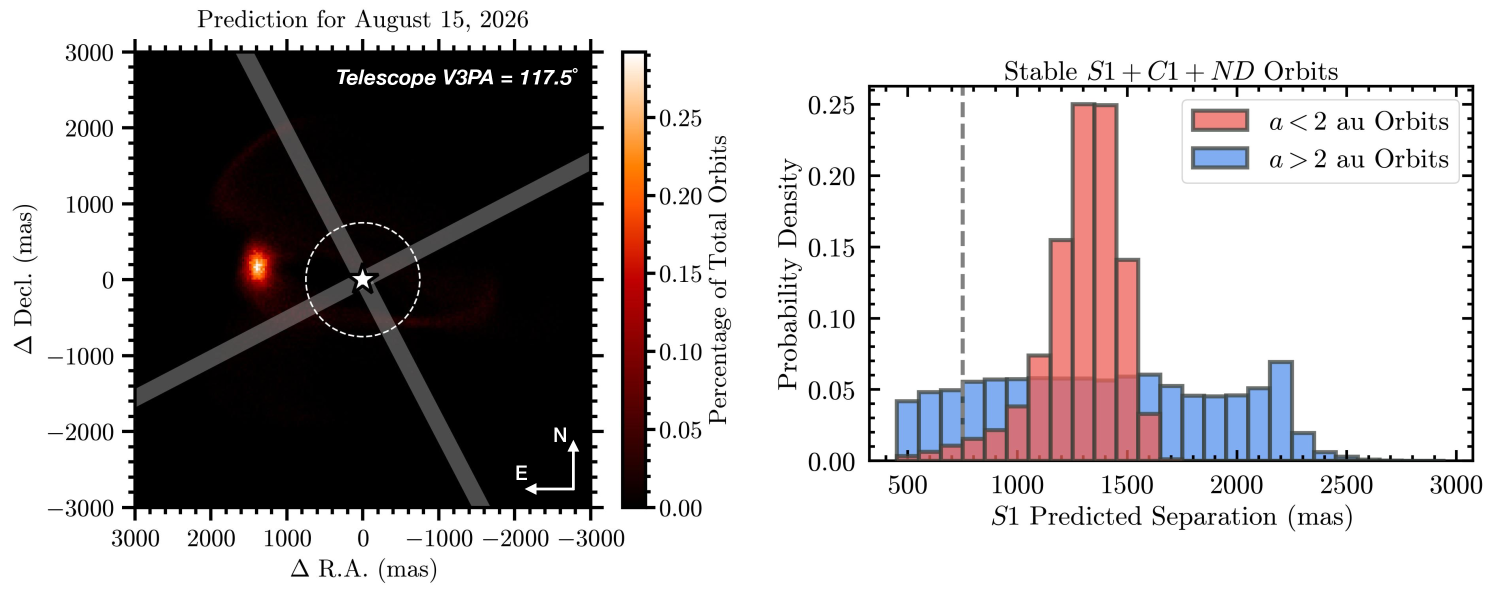
The most pressing task for further work is to capture a second sighting of with JWST. Figure 19 identifies an excellent opportunity in August 2026 to recover based on the family of stable orbits consistent with non-detections described in 4. Around this date, the separation exceeds 1″ and the predicted location is clear of the 4QPM boundaries. There is an urgency to this given the rapid approach of Cen A to the known background star denoted KS5 (Kervella et al., 2016). Between mid-2027 and mid-2028, the two will be within 3″ of one another. Additionally, there are numerous opportunities to follow-up the detection of the candidate exoplanet for further characterization with upcoming and future facilities:
- •
-
•
The coronagraphic instrument on the Nancy Roman Space Telescope has a mask specifically designed to work in the presence of a binary star system (Bendek et al., 2021) and could be used to detect reflected visible light from a gas giant around 1–2 au.
-
•
The METIS instrument on the European Extremely Large Telescope (EELT) should be capable of spectroscopic observations of the candidate (Birkby & Parker, 2024) and could even look for radial velocity shifts in the motion of the planet due to the presence of an exomoon.
-
•
Direct mass measurements should be possible with additional RV monitoring and with differential astrometry at millimeter wavelengths with ALMA (Akeson et al., 2021), or at visible wavelengths with the proposed Toliman (Tuthill et al., 2018) or SHERA (J. Christiansen, private comm.) space telescopes.
-
•
Finally, the proposed Habitable Worlds Observatory (HWO) could, if equipped with appropriate binary star rejection capabilities, search for terrestrial-sized planets which might be found within the Cen A system despite the pessimistic concerns about the stability of orbits exterior to 0.4 au (6.1.2).
7 Conclusions
We conducted JWST/MIRI F1550C coronagraphic imaging observations of the nearest solar-type star, Centauri A, over three epochs between August 2024 and April 2025 to directly resolve Cen A’s habitable zone and perform a deep search for planets and exozodiacal disk emission. The key results from our program are summarized below.
Detection of a candidate gas giant exoplanet in orbit around our nearest Sun-like star, Cen A. We detected a point source () in the August 2024 epoch of JWST/MIRI 15.5 m coronagraphic imaging. Detailed analysis, including various tests, presented in Paper II (Sanghi & Beichman et al., 2025) show that the source is unlikely to be a detector or speckle artifact. We definitively show that is neither a foreground nor a background object. However, with only a single sighting by JWST, the candidate cannot be unambiguously confirmed as a bona fide planet.
Deep upper limits on an exozodiacal disk around Cen A. These observations have set stringent upper bounds on the presence of extended “exozodiacal” dust disk in the habitable zone of Cen A. A limit of 5–8 the dust level within our own zodiacal cloud (for a disk coplanar with the Cen AB orbit) is a factor of 5–10 more sensitive than those set by either photometric or interferometric methods toward more distant stars. Simulations show that for a planet with the candidate’s properties, it is unlikely that a debris disk could remain stable and survive the planet’s dynamical influence unless located within 0.4 au of the star.
Orbital properties of the Cen A planet candidate. By linking the sighting of JWST/MIRI to another candidate, , detected by the VLT/NEAR experiment in 2019, we found a set of dynamically stable orbits. 52% of the stable orbits were consistent with a non-detection of the planet candidate in the February and April 2025 epochs, indicating that it was likely missed in both follow-up observations due to orbital motion. The candidate is in a highly inclined (50∘ or 130∘ with respect to the Cen AB binary orbital plane) and eccentric () orbit, not unlike other S-type planets in close binary systems (e.g., HD 196885 Ab and Cep Ab), and is expected to undergo large amplitude von Zeipel-Kozai-Lidov (vZKL) oscillations.
Physical properties of the Cen A planet candidate. ’s effective temperature is set by heating from Cen A and is expected to be 225 K based on the candidate’s orbital properties. We found plausible atmospheric model solutions to the photometry for a planet radius between 1.1–1.15 and mass between 90–150 (consistent with RV limits). Alternatively, we showed that a simplified optically thick ring with a cross-section equivalent to half of Saturn’s ring could increase the mid-infrared flux of a smaller ( ) planet to explain the estimated photometry.
Importance of a confirmed planet around Cen A. A confirmation of the candidate as a gas giant planet orbiting our closest solar-type star, Cen A, would present an exciting new opportunity for exoplanet research. Such an object would be the nearest (1.33 pc), coldest (225 K), oldest (5 Gyr), shortest period (2–3 years), and lowest mass ( 200 ) planet imaged in orbit around a solar-type star, to date. Its extremely cold temperature would make it more analogous to our own gas giant planets and an important target for atmospheric characterization studies. Its very existence would challenge our understanding of the formation and subsequent dynamical evolution of planets in complex hierarchical systems. Future observations will confirm or reject its existence and then refine its mass and orbital properties, while multi-filter photometric and, eventually, spectroscopic observations will probe its physical nature.
Appendix A Details of the Observation Strategy
| R.A. | R.A.aaCombined uncertainty from parallax and proper motion between 2016.0 and 2024.3. | Decl. | Decl.bbFlux density measured in June 2023 test images. | ||
|---|---|---|---|---|---|
| Date | JD | (deg) | (sec) | (deg) | (″) |
| 8/10/2024 | 2460750.363 | 219.84748601 | (23.3967) | 60.83161739 | (53.8226) |
| 2/20/2025 | 2460727.234 | 219.8472157 | (23.3318) | 60.8317325 | (54.2370) |
| 4/25/2025 | 2460790.995 | 219.8464966 | (23.1592) | 60.83177278 | (54.3820) |
| 4/25/2025 | 2460791.2344 | 219.8464935 | (23.1584) | 60.8317725 | (54.3813) |
Note. — aRelative to 39m. bRelative to 49′. Positions incorporate proper motion and parallax as seen from vantage point of JWST.
| Star | Gaia ID | R.A. | Decl. | R.A. | Decl. | Parallax | Total UncertaintyaaCombined uncertainty from parallax and proper motion between 2016.0 and 2024.3. | Fν(F1000W)bbFlux density measured in June 2023 test images. |
|---|---|---|---|---|---|---|---|---|
| (deg, 2016.0) | (deg, 2016.0) | (mas yr-1) | (mas yr-1) | (mas) | (mas) | (Jy) | ||
| Mus | 5859405805013401984 | 184.3887799 | 67.960909 | 2.68 | ||||
| Mus TAccOffset star used for target acquisition (TA) of Mus in all three epochs. (G9) | 5859405804986931200 | 184.3941452 | 67.953630 | 0.21 | 13450 | |||
| Cen TAddOffset star used for target acquisition (TA) of Cen A in August 2024 and February 2025. (G0) | 5877725249280411392 | 219.8776270 | 60.828383 | 1.28 | 1350 | |||
| Cen TAeeOffset star used for target acquisition (TA) of Cen A in April 2025. (G5) | 5877725146201190144 | 219.8800796 | 60.8445635 | 0.23 | 580 |
| PID-Obs. # | Target | # Dither | Science Time | Start Time | Observation Mid-Point | MIRI (X,Y) OffsetsaaOffsets from the Gaia star to the target star were calculated based on the epoch positions using the STScI software pysiaf. |
|---|---|---|---|---|---|---|
| (hr) | (UTC) | (UTC) | (arcsec) | |||
| 1618-11 | Cen Snapshot (F1000W)bbThe F1000W broadband image was obtained with FASTR1 using 60 groups. | 4 | 0.19 | 06/19/2023 10:00 | ||
| 1618-50 | Mus Snapshot (F1000W)bbThe F1000W broadband image was obtained with FASTR1 using 60 groups. | 4 | 0.19 | 06/19/2023 10:00 | ||
| 1618-61 | Mus Snapshot (F1550C) | 1 | 0.04 | 07/07/2024 22:31 | ||
| 1618-62 | Cen Snapshot (F1550C) | 1 | 0.04 | 07/08/2024 00:29 | ||
| 1618-63 | Mus Background (F1550C) | 1 | 0.04 | 07/08/2024 02:21 | ||
| 1618-64 | Cen Background (F1550C) | 1 | 0.04 | 07/08/2024 02:52 | ||
| 1618-52 | Mus Visit 1 (V3=135.0∘) | 9 | 7.19 | 08/11/2024 13:00 | 08/11/2024 17:04 | (, ) |
| 1618-53 | Mus Visit 1 Background | 1 | 0.80 | 08/11/2024 21:16 | ||
| 1618-56 | Alpha Cen Roll 2 (V3=112.7∘) | 1 | 2.50 | 08/12/2024 04:56 | 8/12/2024 06:32 | (, ) |
| 1618-57 | Alpha Cen Visit 2 Background | 1 | 2.50 | 08/12/2024 08:09 | ||
| 1618-65 | Mus at Cen B (V3=135∘) | 1 | 0.80 | 08/12/2024 17:11 | 08/12/2024 18:48 | (, ) |
| 6797-01 | Mus Visit 1 (V3=133.0∘) | 9 | 7.19 | 02/20/2025 01:00 | 02/20/2025 04:57 | (, ) |
| 6797-02 | Mus Visit 1 Background | 1 | 0.80 | 02/20/2025 09:04 | ||
| 6797-03 | Mus at Cen B | 1 | 0.80 | 02/20/2025 10:13 | 02/20/2025 11:42 | (, ) |
| 6797-06 | Cen Roll 2 (V3=294.5∘) | 1 | 2.50 | 02/20/2025 19:51 | 02/20/2025 21:20 | (, ) |
| 6797-07 | Cen Roll 2 Background | 1 | 2.50 | 02/20/2025 23:10 | ||
| 6797-08 | Mus Visit 2 (V3=133.0∘) | 9 | 7.19 | 02/21/2025 02:17 | 02/21/2025 06:15 | (, ) |
| 6797-09 | Mus Visit 2 Background | 1 | 0.80 | 02/21/2025 10:22 | ||
| 6797-10 | Mus at Cen B (V3=133.0∘) | 1 | 2.50 | 02/21/2025 11:30 | 02/21/2025 13:00 | (, ) |
| 9252-01 | Mus Visit 1 (V3=38.0∘) | 9 | 7.19 | 04/25/2025 01:00 | 04/25/2025 04:57 | (, ) |
| 9252-02 | Mus Visit 1 Background | 1 | 0.80 | 04/25/2025 09:04 | ||
| 9252-03 | Mus at Cen B | 1 | 0.80 | 04/25/2025 10:13 | 04/25/2025 11:42 | (, ) |
| 9252-04 | Cen Roll 1 (V3=346∘) | 1 | 2.50 | 04/25/2025 13:35 | 04/25/2025 15:04 | (, ) |
| 9252-05 | Cen Roll 1 Background | 1 | 2.50 | 04/25/2025 16:53 | ||
| 9252-06 | Cen Roll 2 (V3=356∘) | 1 | 2.50 | 04/25/2025 19:51 | 04/25/2025 21:20 | (, ) |
| 9252-07 | Cen Roll 2 Background | 1 | 2.50 | 04/25/2025 23:10 | ||
| 9252-08 | Mus Visit 2 (V3=38.0∘) | 9 | 7.19 | 04/26/2025 02:17 | 04/26/2025 06:15 | (, ) |
| 9252-09 | Mus Visit 2 Background | 1 | 0.80 | 04/26/2025 10:22 | ||
| 9252-10 | Mus at Cen B (V3=38.0∘) | 1 | 2.50 | 04/26/2025 11:30 | 04/26/2025 13:00 | (, ) |
Note. — All F1550C coronagraphic data was obtained with FASTR1 using 30 groups with 400 integrations for Mus (behind the 4QPM) and 1250 integrations for Cen A (behind the 4QPM) and Mus at the off-axis position of Cen B. Observations 1618-1 to 1618-8 were obtained on 07/26/2023 and 07/27/2023 but failed due to either a guide star issues or incorrect offsets from the Gaia stars. Observations 1618-54 and 1618-58 in August 2024 and 6797-04 in February 2025 failed due to guide star issues.
A.1 Reference Star Selection
For stars as bright as Cen A ([F1550C] 1.51 mag), the selection of reference stars is limited. The IRAS Low Resolution Spectrometer (LRS) Catalog (Olnon et al., 1986) was used to identify potential reference stars: m) 50 Jy within 20∘ of Cen A, clean Rayleigh-Jeans photospheric emission, constant ratio (10%) of LRS brightness () across the F1550C band, a low probability of variability during the 300 day IRAS mission (VAR %), and no bright companions within 100″. These criteria resulted in the selection of Mus ([F1550C] = mag), a long period variable star located 17∘ away on the sky with a band variability 0.5 mag (Murakami et al., 2007; Tabur et al., 2009). The ratio of the LRS spectra of the (unresolved) Cen AB system to these stars is constant across the F1550C bandpass to 1% which means that the effects of wavelength mismatches in the reference star subtraction will be negligible.
A.2 Target Acquisition
A.2.1 Astrometry of Cen and Mus
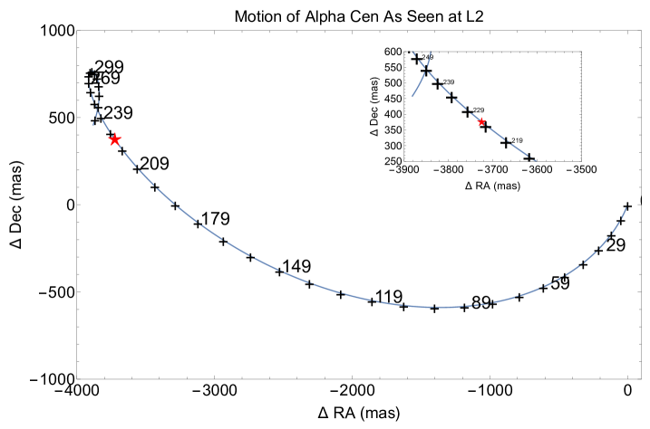
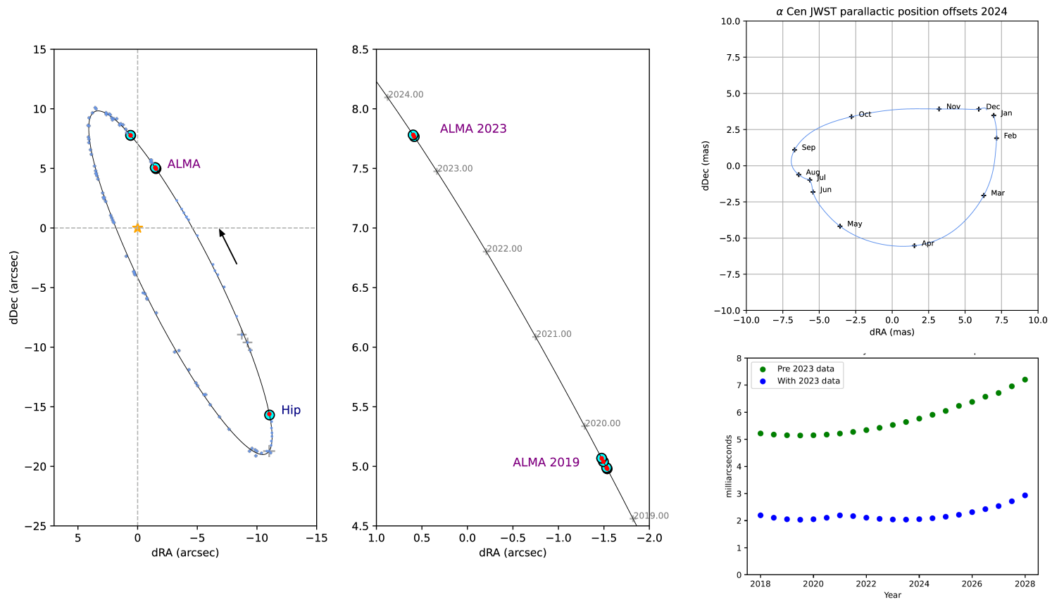
The Cen AB system has a parallax of 750 mas and an annual proper motion of (3640, 700) mas yr-1, which corresponds to a mean motion of 10 mas/day. The description of the procedures leading to the detailed ephemeris used for the observations are provided in Akeson et al. (2021). As described in Appendix B, the ephemeris is based on a combination of absolute astrometry from Hipparcos and ALMA. Radial velocity observations of both Cen A and Cen B help determine the motions of Cen AB in their 80 year orbit. The ephemeris was calculated on an hour-by-hour basis, including the effects of parallax as observed from the vantage point of JWST’s L2 orbit (Figure 20). The location of JWST at L2, an additional 1.5 million km from Earth, increases the parallactic effect by 1% or 7.5 mas, but in a non-intuitive manner due to JWST’s motion at L2 (Figure 21). This effect is not negligible compared to the mas angular diameter of Cen A (Kervella et al., 2017) and the centering accuracy requirement (10 mas) for best performance behind the MIRI coronagraphic mask (Boccaletti et al., 2022).
The precise location of JWST at the epoch of these observations was obtained from the JPL Horizons website999https://ssd.jpl.nasa.gov/horizons/app.html/. The combination of visible data and two epochs of ALMA data (2018/2019 from Akeson et al., 2021) and the 2023 ALMA DDT observations (described in Appendix B.1) for Cen AB yields a precision of 2 mas in the predicted position of Cen A (Figure 21 and Table 6). Taking into account the astrometric precision of the Gaia stars and of Cen itself, we estimate that the overall astrometric precision of the blind offset between the offset stars and the two targets, Mus and Cen A, will be 2.5 mas (), to which must be added the 5–7 mas (1, one axis) offsetting precision of JWST itself101010https://jwst-docs.stsci.edu/jwst-observatory-characteristics/jwst-pointing-performance. Astrometry for Mus, its associated Gaia offset star, and Cen A’s associated Gaia offset star was obtained from the Gaia DR3 catalog (Table 7). The effects of the proper motion and parallax values were taken into account but were relatively minor compared to those for Cen A.
In planning the observational sequences in APT, we specified the exact V3 rotation angles (with a precision of 0.001∘) for each observation and used that information to derive the shift from the Gaia offset star to either Cen A or Mus in instrument coordinates. For Cen A, these calculations used the position of Cen A (including proper motion, parallax and other smaller effects; Akeson et al., 2021) at the expected midpoint of the observation based on a detailed timeline of each observation (Table 8). The small amount of smearing during the 2.8 hr duration of each Cen A observation (2 mas) was deemed acceptable compared to the complexity of designating Cen A as a moving target. The conversion of the offset in to instrument was calculated for the exact epoch of observation and desired V3 angle using a model of the MIRI focal plane using STScI’s pysiaf routine111111https://github.com/spacetelescope/pysiaf.
A.2.2 Offset Star Selection and Validation
The offset stars used for Target Acquisition were drawn from the Gaia DR3 catalog and had to have a mid-IR brightness suitable for easy measurement in a short TA observation. A preliminary search of DR3 revealed 92 targets within 60″ of Cen A and 24 within 30″ of Mus. Cuts in magnitude ( 16 mag) and the requirement that each star have a quoted parallax and proper motion measurement reduced the number to a handful for each source. However, the proximity of both Cen and Mus to the Galactic Plane ( and , respectively) means that the effects of extinction can make predictions of mid-IR brightness highly uncertain. For this reason, we scheduled test observations of both Cen and Mus in the MIRI TA filter (F1000W) without any associated coronagraphic observations. These were executed in June 2023. Figure 1 shows images of Cen and Mus. Simulations using STPSF were developed to assess the influence of the bright target stars ( Cen A, Cen B, and Mus) to ensure that diffraction effects would not affect the detectability of the much fainter Gaia stars in the TA procedure. The star denoted G0 was suitable for both of the V3 roll angles selected for August 2024 and February 2025 (Table 7). The star denoted G5 was used for April 2025. A single star (G9) was suitable for use with Mus at its V3 angle of observation in all three epochs.
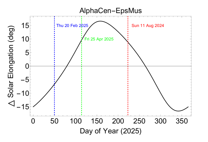
A.3 Minimizing Effects of Telescope Slews
The ability to detect faint companions is dominated by the stability of the wavefront of the JWST telescope and the accurate placement of the star behind the coronagraphic mask. Pre-launch expectations were that there would be slow-varying wavefront error (WFE) drifts 10 nm depending on changes in solar elongation (and thus in the telescope’s thermal balance) and due to stresses from internal structures such as the “frill” surrounding the primary mirror (Perrin et al., 2018). On-orbit performance proved to be significantly better than pre-launch estimates, particularly as the telescope assembly continued to stabilize thermally, with drifts as low as 2–5 nm as measured using semi-daily WFE monitoring observations (Rigby et al., 2023; Lajoie et al., 2023). One factor in selecting the requested observing window was minimizing the change in solar elongation angle between Cen and Mus. The final scheduled dates in August 2024, February 2025, and April 2025 resulted in changes in the absolute value of solar angle (Figure 22). To mitigate further the effects of wavefront drift, we bracketed observations of Cen with observations of Mus. This choice provided redundancy against any failure during guide star and target acquisition by the telescope and thus would still leave one valid PSF reference star observation. Indeed, this proved to be important for the August 2024 observations where one Mus reference observation failed.
A.4 Mitigating the Effects of Cen B
We initially considered strategies either using Cen B as a reference star for Cen A or placing Cen B along the quadrant boundaries of the 4QPM to suppress its starlight. Both strategies had significant disadvantages. In the former case, the brighter star Cen A would be unocculted on the detector in the reference images. In the latter case, very few opportunities were available to schedule observations in the desired configuration. Furthermore, small errors in the position of Cen B along the boundaries would lead to substantial stellar leakage and changes in the PSF. Our pre-launch simulations and current data analysis demonstrated that the influence of Cen B at 7″–9″ separation is sufficiently large in the 1″–2″ region around Cen A that it is necessary to subtract the image obtained by placing Mus, unocculted but through the F1550C mask, at the same offset of Cen B relative to Cen A to provide an off-axis PSF reference. Analysis with the test observations obtained in July 2024 showed that the use of STPSF models was inadequate to remove speckles from Cen B at the required level.
A.5 Mitigation of MIRI Background: The “Glow Sticks”
Following practice recommended by STScI to mitigate the effects of the “Glow Stick” phenomenon (excess telescope background scattered off of telescope structure; Boccaletti et al., 2022; Carter et al., 2023), we included MIRI background observations in exactly the same detector and instrument setup as the on-target observations for both Mus and Cen. These background observations were placed in positions which appeared relatively blank in Spitzer or WISE images. Each background field was observed twice for each object (Table 8) with 5″ shifts in the center position to help mitigate the effects of sources in the fields.
Appendix B Astrometry of the Cen System
Determining the astrometric properties of the Cen system is complex due to the proximity of Cen to Earth and the orbits of the two stars around their common center of mass. High precision visible light observations are scarce due to the brightness of the two stars relative to much fainter reference stars. Akeson et al. (2021) made millimeter-wavelength observations of Cen AB using the ALMA array. At these wavelengths, the two stars are bright enough to yield high SNR data with milli-arcsec precision in an hour of observing time with absolute positions on the ICRF reference frame. The ALMA observations are described in B.1 and the astrometric information used for the JWST observations in B.2.
| Date | Start Time | Star | R.A. | Decl. |
|---|---|---|---|---|
| (UT hours) | ||||
| 01 June 2023 | 02:35 | A | 219.864944115∘ (3 mas) | 60.848591790∘ (3 mas) |
| B | 219.865261605∘ (4 mas) | 60.846446520∘ (4 mas) | ||
| AB | 05935 00004 | 76756 00005 | ||
| 17 June 2023 | 01:55 | A | 219.850279410∘ (1 mas) | 60.831926083∘ (1 mas) |
| B | 219.850610280∘ (1 mas) | 60.829773243∘ (1 mas) | ||
| AB | 05806 00005 | 77502 00005 | ||
| 26 June 2023 | 00:59 | A | 219.850180635∘ (0.8 mas) | 60.831902697∘ (1.1 mas) |
| B | 219.850518885∘ (1.2 mas) | 60.829745590∘ (1.2 mas) | ||
| AB | 05715 00020 | 77234 00020 |
B.1 New ALMA Astrometry of Cen AB
The positions of Cen A and Cen B were observed with ALMA between 2018 Oct 14 and 2019 Aug 26 using about 40 25-m antennas as described in detail in Akeson et al. (2021) and summarized here. The average observing frequency was 343.5 GHz, but the ALMA configurations varied and produced a resolution of 140, 33, 28, 62, and 62 mas for the five observing blocks. Each block was about 80 min long and consisted of about 120 scans of which 15% included calibration sources. The pointing center of each experiment was located near the expected barycenter of the A and B stars to minimize errors caused by small antenna pointing offsets. The Cen AB positions were determined using the phase referencing technique with the nearby quasar, J1452-6502, with an ICRF position accuracy 0.5 mas. This uncertainty produced the main limit to the absolute radio position of the AB system. However, the separation of the A and B stars do not depend on the quasar position accuracy and some of the atmospheric position jitter between the A and B stars also canceled. Further details of the reduction, imaging and multi-calibrator checks to the astrometric accuracy are given in Akeson et al. (2021).
| Julian Year | Time | R.A. ( Cen A) | Decl. ( Cen A) | R.A. ( Cen B) | Decl. ( Cen B) | (AB) | (AB) |
|---|---|---|---|---|---|---|---|
| (J2000, deg) | (J2000, deg) | (J2000, deg) | (J2000, deg) | (arcsec) | (deg, North ) | ||
| 2024.0000000 | 2024-01-01T12:00:00.000 | 219.84969992 | 60.83174299 | 219.85019709 | 60.82949888 | 8.1258 | 6.1630 |
| 2024.0027379 | 2024-01-02T12:00:00.000 | 219.84969758 | 60.83174528 | 219.85019558 | 60.82950072 | 8.1275 | 6.1721 |
| 2024.0054757 | 2024-01-03T12:00:00.000 | 219.84969512 | 60.83174758 | 219.85019396 | 60.82950258 | 8.1293 | 6.1812 |
| 2024.0082136 | 2024-01-04T12:00:00.000 | 219.84969256 | 60.83174989 | 219.85019224 | 60.82950444 | 8.1310 | 6.1903 |
| 2024.0109514 | 2024-01-05T12:00:00.000 | 219.84968989 | 60.83175221 | 219.85019041 | 60.82950632 | 8.1328 | 6.1994 |
Note. — The coordinates are apparent coordinates from the location of JWST. The astrometry is available at10.5281/zenodo.16280658 (catalog 10.5281/zenodo.16280658).
New observations were obtained through an accepted ALMA DDT proposal on 2023 June 1, 17 and 26 (DDT proposal 2022.A.00017.S). The data were taken in Band 7 (343.5 GHz) with the correlator configured for maximum broadband sensitivity. The 2023 positions are listed in Table 1 and were derived from pipeline-processed data using additional analysis to determine the internal position uncertainties. Due to the large proper motion of Cen, roughly 10 mas/day on average, the phase center tracking has a significant impact on the measured positions. For the 2023 June 1 observations, the Cen A position was tracked with time, while for the 2023 June 17 and 26 observations, the phase center was located near Cen A, but was not tracked with time.
The main improvement from the previous ALMA observations (Akeson et al., 2021) is the measurement of internal position errors. These were estimated by splitting each 50-min experiment into three independent parts and then determining the mean stellar position and the error from the scatter among the three parts. The slight stellar motion during an hour observation (0.4 mas) is much less than that caused by the typical temporal “atmospheric” variations. For the 2023 June 17 and 26 observations, where the phase center was located near Cen A, but was not tracked with time, the Cen A and Cen B 1-sigma position errors are about 1.5 mas. For the 2023 June 1 observation, during which the Cen A position was phased tracked, the location of the absolute frame of the images is uncertain, resulting in a larger absolute position error estimate (Table 1).
The absolute star positions in the DDT observations are tied to the phase calibrator (J1408-5712) whose absolute position is measured by global VLBI observations. Its absolute position has an uncertainty of about 1.5 mas which is, unfortunately, relatively large for an ICRF source since it has not been observed very often. The calibrator is located only 5.4∘ away from Cen and is the closest of the brighter available calibrators. If the J1408-5712 position error and the Cen A internal position errors are combined, then the ICRF absolute position errors should be no larger than 2 mas in R.A. and in Decl.
The separation of Cen A and Cen B was also obtained for these observations, again by splitting up each 50-min experiment into three parts. The estimated separation error is less than 1 mas for the 2023 June 17 and 26 observations because much of the error that affect the absolute position of A and B cancels when calculating the stellar position difference. The accuracy is mostly signal-to-noise limited. Since the A–B separation for the 2023 June 1 observation does not depend on the somewhat uncertain definition of the absolute coordinate grid, its accuracy is only a bit larger than the two later observations.
B.2 Astrometry of Cen A, Cen B and Cen AB
The analysis method for determining the astrometric properties of the Cen AB system using the combined visible and ALMA data is described in Akeson et al. (2021). The updated orbit is visualized in Figure 21. Accurate knowledge of the position of Cen A depends on accounting for the location of JWST at L2. The differences in the parallactic motion between the two observing sites, Earth and L2 is 5 mas (Figure 21). Finally, we note that the addition of the ALMA DDT observations reduced the uncertainty in the positions of Cen A from 5–6 mas to 2 mas through 2028 (Figure 21). A detailed analysis of the orbit of Cen AB, including all ALMA epochs and new HARPS radial velocity data will be presented in a forthcoming paper (Kervella et al., in prep).
Table 2 lists the position of Cen A and Cen B as seen from JWST’s location (which is obtained from the HORIZONS database121212https://ssd.jpl.nasa.gov/horizons/app.html/) and lists the relative positions of Cen A and Cen B, which were used in positioning the reference star Mus at the position of Cen B to mitigate the speckles from the unocculted star. The first few entries of the full ephemeris are displayed and the complete table is available in electronic form at10.5281/zenodo.16280658 (catalog 10.5281/zenodo.16280658).
References
- Akeson et al. (2021) Akeson, R., Beichman, C., Kervella, P., et al. 2021, AJ, 162, 14. doi:10.3847/1538-3881/abfaff
- Astropy Collaboration et al. (2022) Astropy Collaboration, Price-Whelan, A. M., Lim, P. L., et al. 2022, ApJ, 935, 167
- Batalha et al. (2019) Batalha, N. E., Marley, M. S., Lewis, N. K., and Fortney, J. J. 2019 ApJ, 878, 1, 70. doi:10.3847/1538-4357/ab1b51
- Bayo et al. (2008) Bayo, A., Rodrigo, C., Barrado Y Navascués, D., et al. 2008, A&A, 492, 277. doi:10.1051/0004-6361:200810395
- Beichman et al. (2005) Beichman, C. A., Bryden, G., Rieke, G. H., et al. 2005, ApJ, 622, 2, 1160. doi:10.1086/428115
- Beichman et al. (2020) Beichman, C., Ygouf, M., Llop Sayson, J., et al. 2020, PASP, 132, 015002
- Beiler et al. (2024) Beiler, S. A., Mukherjee, S., Cushing, M. C., et al. 2024, ApJ, 973, 1, 60. doi:10.3847/1538-4357/ad6759
- Bendek et al. (2021) Bendek, E. A., Belikov, R., Sirbu, D., et al. 2021, Proc. SPIE, 11823, 1182311. doi:10.1117/12.2594992
- Birkby & Parker (2024) Birkby, J. & Parker, L. 2024, AAS/Division for Extreme Solar Systems Abstracts, 56, 503.01
- Blunt et al. (2017) Blunt, S., Nielsen, E. L., De Rosa, R. J., et al. 2017, AJ, 153, 229. doi:10.3847/1538-3881/aa6930
- Blunt et al. (2020) Blunt, S., Wang, J. J., Angelo, I., et al. 2020, AJ, 159, 89. doi:10.3847/1538-3881/ab6663
- Boccaletti et al. (2015) Boccaletti, A., Lagage, P.-O., Baudoz, P., et al. 2015, PASP, 127, 633
- Boccaletti et al. (2022) Boccaletti, A., Cossou, C., Baudoz, P., et al. 2022, A&A, 667, A165. doi:10.1051/0004-6361/202244578
-
Brooke (2003)
Brooke, T. Y. “Main Belt Asteroids in Spitzer Observations”, 2003, https://irsa.ipac.caltech.edu/
data/SPITZER/docs/files/spitzer/asteroid_memo.pdf - Buser & Kurucz (1992) Buser, R. & Kurucz, R. L. 1992, A&A, 264, 557
- Bushouse et al. (2022) Bushouse, H., Eisenhamer, J., Dencheva, N., et al. 2022, JWST Calibration Pipeline, Zenodo, doi:10.5281/ZENODO.7038885. https://zenodo.org/record/7038885
- Brandt (2024) Brandt, T. D. 2024, PASP, Optimal Fitting and Debiasing for Detectors Read Out Up-the-Ramp, 136, 4, 045004. doi:10.1088/1538-3873/ad38d9
- Butler et al. (2004) Butler R. P., Bedding T. R., Kjeldsen H., McCarthy C., O’Toole S. J., Tinney C. G., Marcy G. W., et al., 2004, ApJL, 600, L75. doi:10.1086/381434
- Carter et al. (2023) Carter, A. L., Hinkley, S., Kammerer, J., et al. 2023, ApJ, 951, L20. doi:10.3847/2041-8213/acd93e
- Carter et al. (2025) Carter, A., Kammerer, J., Leisenring, J., et al. 2025, Astrophysics Source Code Library, spaceKLIP: JWST coronagraphy data data reduction and analysis pipeline. ascl:2502.014
- Castelli & Kurucz (2003) Castelli, F. & Kurucz, R. L. 2003, Modelling of Stellar Atmospheres, 210, A20. doi:10.48550/arXiv.astro-ph/0405087
- Chauvin et al. (2023) Chauvin, G., Videla, M., Beust, H., et al. 2023, A&A, 675, A114. doi:10.1051/0004-6361/202244502
- Christiansen et al. (2025) Christiansen, J. L., McElroy, D. L., Harbut, M., et al. 2025, , arXiv:2506.03299. doi:10.48550/arXiv.2506.03299
- Clarke (1986) Clarke, Arthur. C. 1986 The Songs of Distant Earth, Del Rey Books (US), 1986, ISBN:0-345-33219-9
- Coulter et al. (2022) Coulter, D. J., Barnes, J. W., & Fortney, J. J. 2022, ApJS, Jupiter and Saturn as Spectral Analogs for Extrasolar Gas Giants and Brown Dwarfs, 263, 1, 15. doi:10.3847/1538-4365/ac886a
- Cuello & Sucerquia (2024) Cuello, N. & Sucerquia, M. 2024, Universe, 10, 2, 64. doi:10.3390/universe10020064
- Crotts et al. (2025) Crotts, K. A., Carter, A. L., Lawson, K., et al. 2025, , arXiv:2506.19932. doi:10.48550/arXiv.2506.19932
- Dohnanyi (1969) Dohnanyi, J. S. 1969, J. Geophys. Res., 74, 2531. doi:10.1029/JB074i010p02531
- Ducati (2002) Ducati, J. R. 2002, VizieR Online Data Catalog
- Dupuy et al. (2022) Dupuy, T. J., Kraus, A. L., Kratter, K. M., et al. 2022, MNRAS, 512, 648. doi:10.1093/mnras/stac306
- Dupuy et al. (2016) Dupuy, T. J., Kratter, K. M., Kraus, A. L., et al. 2016, ApJ, 817, 80. doi:10.3847/0004-637X/817/1/80
- Lester et al. (2023) Lester, K. V., Dupuy, T. J., Kraus, A. L., et al. 2023, AJ, 166, 166. doi:10.3847/1538-3881/acf167
- Engels et al. (1981) Engels, D., Sherwood, W. A., Wamsteker, W., et al. 1981, A&AS, 45, 5
- Ertel et al. (2018) Ertel, S., Defrère, D., Hinz, P., et al. 2018, AJ, 155, 194
- Ertel et al. (2020) Ertel, S., Defrère, D., Hinz, P., et al. 2020, AJ, 159, 177
- Evans et al. (2024) Evans, E. L., Dupuy, T. J., Sullivan, K., et al. 2024, MNRAS, 534, 575. doi:10.1093/mnras/stae2095
- Farihi et al. (2025) Farihi, J., Su, K. Y. L., Melis, C., et al. 2025, ApJ, Subtle and Spectacular: Diverse White Dwarf Debris Disks Revealed by JWST, 981, 1, L5. doi:10.3847/2041-8213/adae88
- Fegley & Prinn (1985) Fegley, B. & Prinn, R. G. 1985, ApJ, Equilibrium and nonequilibrium chemistry of Saturn’s atmosphere - Implications for the observability of PH3, N2, CO, and GeH4., 299, 1067. doi:10.1086/163775
- Feng (2024) Feng, T. 2024, arXiv:2406.19177. doi:10.48550/arXiv.2406.19177
- Feroz et al. (2009) Feroz, F., Hobson, M. P., & Bridges, M. 2009, MNRAS, 398, 4, 1601. doi:10.1111/j.1365-2966.2009.14548.x
- Foreman-Mackey et al. (2013) Foreman-Mackey, D., Hogg, D. W., Lang, D., et al. 2013, PASP, 125, 925, 306. doi:10.1086/670067
- Gaia Collaboration et al. (2016) Gaia Collaboration, Prusti, T., de Bruijne, J. H. J., et al. 2016, A&A, 595, A1. doi:10.1051/0004-6361/201629272
- Harris et al. (2020) Harris, C. R., Millman, K. J., van der Walt, S. J., et al. 2020, Nature, 585, 7825, 357. doi:10.1038/s41586-020-2649-2
- Heppenheimer (1978) Heppenheimer, T. A. 1978, A&A, 65, 421
- Huang & Ji (2022) Huang, X. & Ji, J. 2022, AJ, 164, 5, 177. doi:10.3847/1538-3881/ac8f4c
- Hunter (2007) Hunter, J. D. 2007, Computing in Science and Engineering, 9, 3, 90. doi:10.1109/MCSE.2007.55
- Innanen et al. (1997) Innanen, K. A., Zheng, J. Q., Mikkola, S., et al. 1997, AJ, 113, 1915. doi:10.1086/118405
- Ito & Ohtsuka (2020) Ito, T. & Ohtsuka, K. 2020, European Planetary Science Congress, EPSC2020-269. doi:10.5194/epsc2020-269
- Johnson & McClure (1976) Johnson, R. G. & McClure, B. T. 1976, Quaternary Research, A model for Northern Hemisphere continental ice sheet variation, 6, 3, 325. doi:10.1016/0033-5894(67)90001-4
- Kammerer et al. (2022) Kammerer, J., Girard, J., Carter, A. L., et al. 2022, Proc. SPIE, 12180, 121803N. doi:10.1117/12.2628865
- Kelsall et al. (1998) Kelsall, T., Weiland, J. L., Franz, B. A., et al. 1998, ApJ, The COBE Diffuse Infrared Background Experiment Search for the Cosmic Infrared Background. II. Model of the Interplanetary Dust Cloud, 508, 1, 44. doi:10.1086/306380
- Kennedy et al. (2011) Kennedy, G. M., Wyatt, M. C., Su, K. Y. L., et al. 2011, MNRAS, 417, 2281.
- Kennedy & Wyatt (2013) Kennedy, G. M., & Wyatt, M. C. 2013, MNRAS, 433, 2334
- Kennedy et al. (2015) Kennedy, G. M., Matrà, L., Marmier, M., et al. 2015, MNRAS, Kuiper belt structure around nearby super-Earth host stars, 449, 3, 3121. doi:10.1093/mnras/stv511
- Kervella et al. (2016) Kervella, P., Mignard, F., Mérand, A., & Thévenin, F. 2016, A&A, 594, A107
- Kervella et al. (2017) Kervella, P., Bigot, L., Gallenne, A., et al. 2017, A&A, 597, A137
- Kozai (1962) Kozai, Y. 1962, AJ, 67, 591. doi:10.1086/108790
- Kraus et al. (2016) Kraus, A. L., Ireland, M. J., Huber, D., Mann, A. W., & Dupuy, T. J. 2016, AJ, 152, 8
- Kuchner (2012) Kuchner, M. 2012, Astrophysics Source Code Library,“ZODIPIC: Zodiacal Cloud Image Synthesis”, ascl:1202.002
- Lacy & Burrows (2023) Lacy, B. & Burrows, A. 2023, ApJ, Self-consistent Models of Y Dwarf Atmospheres with Water Clouds and Disequilibrium Chemistry, 950, 1, 8. doi:10.3847/1538-4357/acc8cb
- Lajoie et al. (2023) Lajoie, C.-P., Lallo, M., Meléndez, M., et al. 2023, Technical Report JWST-STScI-008497. doi:10.48550/arXiv.2307.11179
- Leggett et al. (2007) Leggett, S. K., Saumon, D., Marley, M. S., et al. 2007, ApJ, 3.6-7.9 m Photometry of L and T Dwarfs and the Prevalence of Vertical Mixing in their Atmospheres, 655, 2, 1079. doi:10.1086/510014
- Leggett et al. (2021) Leggett, S. K., Tremblin, P., Phillips, M. W., et al. 2021, ApJ, Measuring and Replicating the 1-20 m Energy Distributions of the Coldest Brown Dwarfs: Rotating, Turbulent, and Nonadiabatic Atmospheres, 918, 1, 11. doi:10.3847/1538-4357/ac0cfe
- Leggett & Tremblin (2023) Leggett, S. K. & Tremblin, P. 2023, ApJ, The First Y Dwarf Data from JWST Show that Dynamic and Diabatic Processes Regulate Cold Brown Dwarf Atmospheres, 959, 2, 86. doi:10.3847/1538-4357/acfdad
- Leggett & Tremblin (2024) Leggett, S. K. & Tremblin, P. 2024, Research Notes of the American Astronomical Society, James Webb Space Telescope Spectra of Cold Brown Dwarfs are Well-reproduced by Phosphine-free, Diabatic, ATMO2020++ Models, 8, 1, 13. doi:10.3847/2515-5172/ad1b61
- Leisenring (2024) Leisenring, J. 2024, ApJ, in prep
- Li et al (2018) Li,L., Jiang, X., West, R. A. it Nature Comm., 3709, https://doi.org/10.1038/s41467-018-06107-2
- Lidov (1962) Lidov, M. L. 1962, Planet. Space Sci., 9, 10, 719. doi:10.1016/0032-0633(62)90129-0
- Lightsey et al. (2018) Lightsey, P. A., Knight, J. S., Barto, A., et al. 2018, Proceedings Volume 10698, Space Telescopes and Instrumentation 2018: Optical, Infrared, and Millimeter Wave; 1069804 (2018) https://doi.org/10.1117/12.2312276
- Lissauer et al. (2014) Lissauer, J. J., Marcy, G. W., Bryson, S. T., et al. 2014, ApJ, 784, 44
- Luhman et al. (2024) Luhman, K. L., Tremblin, P., Alves de Oliveira, C., et al. 2024, AJ, JWST/NIRSpec Observations of the Coldest Known Brown Dwarf, 167, 1, 5. doi:10.3847/1538-3881/ad0b72
- Marley et al. (2021) Marley, M. S., Saumon, D., Visscher, C., et al. 2021, ApJ, The Sonora Brown Dwarf Atmosphere and Evolution Models. I. Model Description and Application to Cloudless Atmospheres in Rainout Chemical Equilibrium, 920, 2, 85. doi:10.3847/1538-4357/ac141d
- Mawet et al. (2014) Mawet, D., Milli, J., Wahhaj, Z., et al. 2014, ApJ, 792, 2, 97. doi:10.1088/0004-637X/792/2/97
- Meisner et al. (2023) Meisner, A. M., Leggett, S. K., Logsdon, S. E., et al. 2023, AJ, Exploring the Extremes: Characterizing a New Population of Old and Cold Brown Dwarfs, 166, 2, 57. doi:10.3847/1538-3881/acdb68
- Moe & Kratter (2021) Moe, M. & Kratter, K. M. 2021, MNRAS, 507, 3593. doi:10.1093/mnras/stab2328
- Morley et al. (2014) Morley, C. V., Marley, M. S., Fortney, J. J., et al. 2014, ApJ, Water Clouds in Y Dwarfs and Exoplanets, 787, 1, 78. doi:10.1088/0004-637X/787/1/78
- Mukherjee et al. (2023) Mukherjee, S., Batalha, N. E., Fortney, J. J., and Marley, M. S., 2023 ApJ, 942, 2, 71 doi:10.3847/1538-4357/ac9f48
- Mukherjee et al. (2024) Mukherjee, S., Fortney, J. J., Morley, C. V., et al. 2024, ApJ, 963, 1, 73. doi:10.3847/1538-4357/ad18c2
- Müller et al. (2024) Müller, S., Baron, J., Helled, R., et al. 2024, A&A, 686, A296. doi:10.1051/0004-6361/202348690
- Murakami et al. (2007) Murakami, H., Baba, H., Barthel, P., et al. 2007, PASJ, 59, S369. doi:10.1093/pasj/59.sp2.S369
- Naoz (2016) Naoz, S. 2016, ARA&A, 54, 441. doi:10.1146/annurev-astro-081915-023315
- Noll et al. (1997) Noll, K. S., Geballe, T. R., & Marley, M. S. 1997, ApJ, Detection of Abundant Carbon Monoxide in the Brown Dwarf Gliese 229B, 489, 1, L87. doi:10.1086/310954
- Olnon et al. (1986) Olnon, F. M., Raimond, E., Neugebauer, G., et al. 1986, A&A(S), 65, 607
- Peale & Cassen (1978) Peale, S. J. & Cassen, P. 1978, Icarus, Contribution of tidal dissipation to lunar thermal history, 36, 2, 245. doi:10.1016/0019-1035(78)90109-4
- Perrin et al. (2014) Perrin, M. D., Sivaramakrishnan, A., Lajoie, C.-P., et al. 2014, in Society of Photo-Optical Instrumentation Engineers (SPIE) Conference Series, Vol. 9143, Space Telescopes and Instrumentation 2014: Optical, Infrared, and Millimeter Wave, ed. J. Oschmann, Jacobus M., M. Clampin, G. G. Fazio, & H. A. MacEwen, 91433X
- Perrin et al. (2018) Perrin, M. D., Pueyo, L., Van Gorkom, K., et al. 2018, Proceedings Volume 10698, Space Telescopes and Instrumentation 2018: Optical, Infrared, and Millimeter Wave; 1069809 (2018) https://doi.org/10.1117/12.2313552
- Phillips et al. (2020) Phillips, M. W., Tremblin, P., Baraffe, I., et al. 2020, A&A, A new set of atmosphere and evolution models for cool T-Y brown dwarfs and giant exoplanets, 637, A38. doi:10.1051/0004-6361/201937381
- Planck Collaboration et al. (2016) Planck Collaboration, Ade, P. A. R., Aghanim, N., et al. 2016, A&A, 586, A132. doi:10.1051/0004-6361/201424945
- Polletta et al. (2007) Polletta, M., Tajer, M., Maraschi, L., et al. 2007, ApJ, 663, 81. doi:10.1086/518113
- Quarles & Lissauer (2016) Quarles, B. & Lissauer, J. J. 2016, AJ, 151, 111
- Quarles & Lissauer (2018) Quarles, B., & Lissauer, J. J. 2018, AJ, 155, 130
- Quarles, Lissauer & Kaib (2018) Quarles, B., Lissauer, J. J., & Kaib, N. 2018, AJ, 155, 64
- Quintana et al. (2002) Quintana, E. V., Lissauer, J. J., Chambers, J. E., & Duncan, M. 2002, ApJ, 576, 2. doi:10.1086/341808
- Quirrenbach (2022) Quirrenbach, A. 2022, Research Notes AAS, 6, 3, 56. doi:10.3847/2515-5172/ac5f0d
- Rafikov & Silsbee (2014) Rafikov, R. R., & Silsbee, K. 2014, ApJ, 798, 70. doi:10.1088/0004-637X/798/2/70
- Rieke & Gautier (2004) Rieke, G. & Gautier, N. 2004, Spitzer Proposal, 52
- Rigby et al. (2023) Rigby, J., Perrin, M., McElwain, M., et al. 2023, PASP, 135, 048001. doi:10.1088/1538-3873/acb293
- Rein and Liu (2012) Rein, H. and S.-F. Liu 2012, A&A537 A128.
- Rein et al. (2019) Rein, H., D. Tamayo, and G. Brown 2019, MNRAS489 4632.
- Rieke et al. (2015) Rieke, G. H., Ressler, M. E., Morrison, J. E., et al. 2015, PASP, 127, 665.doi:10.1086/682252
- Sanghi et al. (2025) Sanghi, A., Beichman, C., Mawet, D., et al. 2025, Research Notes of the American Astronomical Society, 9, 5, 119. doi:10.3847/2515-5172/add880
- Sanghi & Beichman et al. (2025) Sanghi, A, Beichman, C.A, et al. 2025, in press.
- Silsbee & Rafikov (2021) Silsbee, K., & Rafikov, R. R. 2021, A&A, 652, A104. doi:10.1051/0004-6361/202141139
- Soummer et al. (2012) Soummer, R., Pueyo, L., & Larkin, J. 2012, ApJ, 755, 2, L28. doi:10.1088/2041-8205/755/2/L28
- STScI Development Team (2013) STScI Development Team 2013, Astrophysics Source Code Library. ascl:1303.023
- Rigley & Wyatt (2020) Rigley, J. K. & Wyatt, M. C. 2020, MNRAS, 497, 1143
- Saumon et al. (2006) Saumon, D., Marley, M. S., Cushing, M. C., et al. 2006, ApJ, Ammonia as a Tracer of Chemical Equilibrium in the T7.5 Dwarf Gliese 570D, 647, 1, 552. doi:10.1086/505419
- Sommer et al. (2025) Sommer, M., Wyatt, M., & Han, Y. 2025, MNRAS, 539, 439. doi:10.1093/mnras/staf494
- Stone et al. (2024) Stone, M. A., Alberts, S., Rieke, G. H., et al. 2024, ApJ, 5–25 m Galaxy Number Counts from Deep JWST Data, 972, 1, 62. doi:10.3847/1538-4357/ad6308
- Su et al. (2013) Su, K. Y. L., Rieke, G. H., Malhotra, R., et al. 2013, ApJ, 763, 118
- Sullivan et al. (2024) Sullivan, K., Kraus, A. L., Berger, T. A., et al. 2024, AJ, 168, 129. doi:10.3847/1538-3881/ad6310
- Tabur et al. (2009) Tabur, V., Bedding, T. R., Kiss, L. L., et al. 2009, MNRAS, 400, 1945. doi:10.1111/j.1365-2966.2009.15588.x
- Teplitz et al. (1999) Teplitz, V. L., Stern, S. A., Anderson, J. D., et al. 1999, ApJ, 516, 425
- Thebault et al. (2021) Thebault, P., Kral, Q., & Olofsson, J. 2021, A&A, 646, A173. doi:10.1051/0004-6361/202039582
- Thebault et al. (2008) Thebault, P., Marzari, F., & Scholl, H. 2008, MNRAS, 388, 1528. doi:10.1111/j.1365-2966.2008.13524.x
- Trilling et al. (2007) Trilling, D. E., Stansberry, J. A., Stapelfeldt, K. R., et al. 2007, ApJ, 658, 1289. doi:10.1086/511668
- Tuthill et al. (2018) Tuthill, P., Bendek, E., Guyon, O., et al. 2018, Proc. SPIE, 10701, 107011J. doi:10.1117/12.2313269
- Valenti & Fischer (2005) Valenti, J. A. & Fischer, D. A. 2005, ApJS, 159, 141. doi:10.1086/430500
- Virtanen et al. (2020) Virtanen, P., Gommers, R., Oliphant, T. E., et al. 2020, Nature Methods, 17, 261. doi:10.1038/s41592-019-0686-2
- von Zeipel (1910) von Zeipel, H. 1910, Astronomische Nachrichten, 183, 22, 345. doi:10.1002/asna.19091832202
- Wang et al. (2015) Wang, J. J., Ruffio, J.-B., De Rosa, R. J., et al. 2015, pyKLIP: PSF Subtraction for Exoplanets and Disks, Astrophysics Source Code Library, record ascl:1506.001.
- Wiegert et al. (2014) Wiegert, J., Liseau, R., Thébault, P., et al. 2014, A&A, 563, A102. doi:10.1051/0004-6361/201321887
- Wagner et al. (2021) Wagner, K., Boehle, A., Pathak, P., et al. 2021, Nature Communications, 12, 922. doi:10.1038/s41467-021-21176-6
- Wogan et al. (2025) Wogan, N. F., Mang, J., Batalha, N. E., et al. 2025, Research Notes of the American Astronomical Society, 9, 5, 108. doi:10.3847/2515-5172/add407
- Wittenmyer et al. (2016) Wittenmyer, R. A., Butler, R. P., Tinney, C. G., et al. 2016, ApJ, 819, 28. doi:10.3847/0004-637X/819/1/28
- Wright et al. (2015) Wright, G. S., Wright, D., Goodson, G. B., et al. 2015, PASP, 127, 595. doi:10.1086/682253
- Wyatt (2005) Wyatt, M. C. 2005, A&A, The insignificance of P-R drag in detectable extrasolar planetesimal belts, 433, 3, 1007. doi:10.1051/0004-6361:20042073
- Wyatt et al. (2007) Wyatt, M. C., Smith, R., Su, K. Y. L., et al. 2007, ApJ, 663, 365. doi:10.1086/518404
- Wyatt et al. (2011) Wyatt, M. C., Clarke, C. J., & Booth, M. 2011, Celestial Mechanics and Dynamical Astronomy, Debris disk size distributions: steady state collisional evolution with Poynting-Robertson drag and other loss processes, 111, 1-2, 1. doi:10.1007/s10569-011-9345-3
- Xuan & Wyatt (2020) Xuan, J. W. & Wyatt, M. C. 2020, MNRAS, 497, 2, 2096. doi:10.1093/mnras/staa2033
- Yelverton et al. (2019) Yelverton, B., Kennedy, G. M., Su, K. Y. L., & Wyatt, M. C. 2019, MNRAS, 488, 3588. doi:10.1093/mnras/stz1927
- Zahnle & Marley (2014) Zahnle, K. J. & Marley, M. S. 2014, ApJ, 797, 1, 41. doi:10.1088/0004-637X/797/1/41
- Zhang & Kainulainen (2022) Zhang, M. & Kainulainen, J. 2022, MNRAS, 517, 5180. doi:10.1093/mnras/stac3012
- Zhang et al. (2024) Zhang, J., Wang, J., Howell, S. B., et al. 2024, AJ, 167, 89. doi:10.3847/1538-3881/ad2152
- Zhao et al. (2018) Zhao, L., Fischer, D. A., Brewer, J., et al. 2018, AJ, 155, 24