Worst-Case Analysis is Maximum-A-Posteriori Estimation
Abstract.
The worst-case resource usage of a program can provide useful information for many software-engineering tasks, such as performance optimization and algorithmic-complexity-vulnerability discovery. This paper presents a generic, adaptive, and sound fuzzing framework, called DSE-SMC, for estimating worst-case resource usage. DSE-SMC is generic because it is black-box as long as the user provides an interface for retrieving resource-usage information on a given input; adaptive because it automatically balances between exploration and exploitation of candidate inputs; and sound because it is guaranteed to converge to the true resource-usage distribution of the analyzed program.
DSE-SMC is built upon a key observation: resource accumulation in a program is isomorphic to the soft-conditioning mechanism in Bayesian probabilistic programming; thus, worst-case resource analysis is isomorphic to the maximum-a-posteriori-estimation problem of Bayesian statistics. DSE-SMC incorporates sequential Monte Carlo (SMC)—a generic framework for Bayesian inference—with adaptive evolutionary fuzzing algorithms, in a sound manner, i.e., DSE-SMC asymptotically converges to the posterior distribution induced by resource-usage behavior of the analyzed program. Experimental evaluation on Java applications demonstrates that DSE-SMC is significantly more effective than existing black-box fuzzing methods for worst-case analysis.
1. Introduction
Software performance testing has always been a significant concern for software developers and testers. With the development of software science, the increase in software complexity drives people to seek for automatic methods. From an industrial point of view, it is routinely requested that units of an algorithms performance should be tested for evaluation and reconstruction. Yet, the process has been from bottom to top for so long that engineers failed to transform it into an automated process. On the other hand, theoretically, it is crucial to notice that, effective as methods based on machine learning now seen, the outcome may be unstable and unreliable in quality.
In common sense, a stable algorithm is one that manages to control its worst-case resource consumption. Generally, developers and testers now utilize fuzzing methods for detecting software vulnerabilities. To achieve better performances, the algorithm should be reliable, stable, and risk-resilient, bringing us to the need for testing. Therefore, it is essential to provide a theory and an applicable approach for generating the worst-case inputs of an algorithm that reveals its potential resource-usage profile objectively, rigorously, and meaningfully.
So far, the number of frameworks in generating the worst-case inputs is relatively limited, compared to fuzzing frameworks. On the one hand, there have been black-box fuzzing-based worst-case-analysis tools such as SlowFuzz (Petsios et al., 2017). Those approaches are generic in the sense that they do not require domain knowledge, but they might be ineffective when the structure of the analyzed program becomes complex. On the other hand, there have been white- and grey-box worst-case-analysis tools, many of which rely on symbolic execution (Burnim et al., 2009; Luckow et al., 2017; Wang and Hoffmann, 2019) or a combination of fuzzing and symbolic execution (Noller et al., 2018). Those approaches turn out to be more effective because they can use information of the concrete implementation of the analyzed program to guide their exploration in the space of candidate worst-case inputs, but they also demand more computational resources to do program analysis, execution-path search, etc.
In this paper, we consider the problem of black-box worst-case analysis. The analysis should be generic, in the sense that it does not require domain- or application-specific knowledge; adaptive, in the sense that it automatically balances between exploration and exploitation of the space of candidate inputs; and sound, in the sense that it correctly accounts for the resource-usage distribution of the analyzed program. The analysis takes a resource-accumulating program (i.e., the program responds with its resource usage under a given metric) and a specification for candidate inputs, generates candidate inputs sequentially and learns from the information revealed in each generation to reach the worst-case resource behavior, and finally outputs an input with as large resource usage as possible.
The major challenge is to actually learn something from the candidate inputs during the generation process, given that the analysis is black-box. Our key observation to solve the challenge is that as our title indicates, there is a correspondence between worst-case analysis (WCA) on resource-accumulating programs and maximum-a-posteriori (MAP) estimation on probabilistic programs. MAP estimation is a well-studied problem in Bayesian inference: it aims to find optimal parameters that maximize the posterior distribution of a probabilistic model, conditioned on observations for the model. Probabilistic programming (Barthe et al., 2020) provides a systematic way of specifying probabilistic models as probabilistic programs, where special soft-conditioning statements account for observations and likelihood accumulation. We thus develop an isomorphism between resource accumulation in an ordinary program and likelihood accumulation in a probabilistic program. Such a correspondence allows us to adapt advances in the field of Bayesian inference, especially MAP estimation, to carry out worst-case analysis.
In this paper, we consider sequential Monte Carlo (SMC), a versatile framework for approximating and optimizing posterior distributions (Del Moral et al., 2006). SMC works by maintaining a set of weighted samples and iteratively evolving them based on observations for the probabilistic model. The workflow of SMC is very similar to evolutionary fuzzing techniques, which maintain a population of candidates and iteratively evolving them via genetic operations such as crossover and mutation. Therefore, we develop Dual-Strategy Evolutionary Sequential Monte-Carlo, abbreviated by DSE-SMC, which incorporates SMC with evolutionary fuzzing. The innovation of DSE-SMC lies in two main aspects. Firstly, we integrate resample-move SMC (Gilks and Berzuini, 2001), which allows using arbitrary Markov-Chain Monte Carlo (MCMC) kernels to evolve the set of samples, with evolutionary MCMC (Drugan and Thierens, 2003), which recasts genetic operations such as crossover and mutation as Monte Carlo methods, and obtain a generic, adaptive, and sound evolutionary SMC framework. Secondly, we introduce a nature-inspired structure of simulating reproduction strategies of organisms (Andrews and Harris, 1986) to strike a balance between exploration and exploitation. The high-level idea is that organisms take different growth strategies in crowded and uncrowded environments: in the former case, they prefer generating a few offspring but with high quality, whereas in the latter case, they prefer generating a lot of offspring mainly for increasing diversity. We implement this idea as a dual-strategy approach, in the sense that DSE-SMC maintains two groups of population, allows them to migrate from each other, and evolves inside each group using a group-specific strategy.
Contributions
The paper’s contributions include the following:
-
•
We establish a correspondence between worst-case analysis (WCA) and maximum-a-posteriori (MAP) by showing how to reduce the WCA problem on a resource-accumulating program to the MAP problem on a probabilistic program, and vice versa (section 2.2).
-
•
We devise DSE-SMC, an SMC-based fuzzing framework for WCA (sections 2.3 and 3).
-
•
We implemented a prototype of DSE-SMC and evaluated it on eight subjects. Our evaluation shows that DSE-SMC is significantly more effective than prior black-box methods (section 4).
section 5 discusses related work. section 6 concludes. LABEL:Se:DataAvailability gives a statement of data availability.
2. Overview
2.1. Problem Statement
In this paper, we analyze the worst-case resource usage of a given application by automatically generating inputs—of some given size—that trigger as large resource usage as possible. We assume that the user of our tool provides an interface to collect resource-usage information from multiple executions of the application, with possibly different inputs. In this way, the user can specify a custom resource metric of interest, e.g., the number of executed program statements, jumps (branches), or method calls. Apart from the input specification and the resource-usage information, we require that our tool be black-box, i.e., it does not have any application-specific knowledge for worst-case analysis. Note that in this paper, our goal is not to estimate asymptotic complexities; instead, we focus on maximizing a user-specified concrete metric over inputs of a given size.
2.2. Worst-Case Analysis is Maximum-A-Posteriori Estimation
To demonstrate our framework, we consider insertion sort as a running example.
For an ordinary implementation of insertion sort, it is well known that its
worst-case time complexity is and its best-case complexity
is , where is the length of the array-to-be-sorted.
Fig. 1(a) presents an implementation of insertion sort
in Java.
To make the resource metric explicit, we interface resource accumulation
with method calls of the form Resource.tick(int).
For the program in Fig. 1(a), the resource metric accounts for
the total number of loop iterations.
For example, if we want to analyze the worst-case resource usage when
the length of the input array is , a worst-case input could be
with a resource usage of loop iterations.
To show how the worst-case analysis (WCA) problem is isomorphic to the maximum-a-posteriori (MAP) estimation, we first review Bayesian inference and probabilistic programming.
-
•
Bayesian inference is a method for inferring the posterior distribution of a probabilistic model conditioned on observed data, with applications in artificial intelligence (Ghahramani, 2015), cognitive science (Griffiths et al., 2008), applied statistics (Gelman et al., 2013), etc. At the core of Bayesian inference is Bayes’ law:
(1) where and are random variables standing for parameters and observations, respectively; is the conditional probability of parameters being given that observations are , i.e., the posterior; is the conditional probability of observations being given that parameters are , i.e., the likelihood; and is the probability of parameters being , i.e., the prior. Because Bayesian inference usually fixes the observations , the denominator of the right-hand side of Eqn. 1 is usually considered as a constant, and thus we can write Eqn. 1 as
(2) Bayesian inference usually accounts for the posterior distribution as a function of given some . People have developed many algorithms to sample from the posterior distribution, e.g., Markov-Chain Monte Carlo (MCMC). In some other scenarios, people have also considered the maximum-a-posteriori (MAP) estimation, i.e., finding an that maximizes the posterior probability .
-
•
Probabilistic programming provides a flexible way of specifying probabilistic models and performing Bayesian inference (Barthe et al., 2020). One way to understand the semantics of a probabilistic program is that it describes the measure that is induced by the product of the likelihood and the prior, i.e., the right-hand side of Eqn. 2. Note that because we ignore the denominator , the product is usually not a probability measure. Consequently, probabilistic programming languages (PPLs)—such as Stan (Carpenter et al., 2017), Pyro (Bingham et al., 2018), Church (Goodman et al., 2008; Goodman and Stuhlmüller, 2014), and Gen (Cusumano-Towner et al., 2019)—have devised many techniques to sample from or approximate unnormalized measures defined by probabilistic programs. A PPL is usually an ordinary programming language with two special extra constructs:
-
–
sampling, which draws a random value from a prior distribution; and
-
–
soft conditioning, which records the likelihood of some observation.
Below gives a simple probabilistic program written as Java pseudocode. The program models a Bayesian-inference task: (i) there is an imprecise scale that responds with a noisy measurement from the Normal distribution when the actual weight is ; (ii) we use the scale to weigh an object and read as the measurement; (iii) we have a prior guess that the object’s weight is around , modeled with the prior distribution ; and (iv) we want to know the posterior distribution of the object’s weight.
1float = Probability.sample(Distribution.Normal(, ));2Probability.observe(, Distribution.Normal(, ));The statement is usally a wrapper around the more primitive statement , where is the likelihood of being sample from ; in this example, we can compute the likelihood using the probability density function of Normal distributions:
A probabilistic program can contain multiple soft-conditioning/scoring statements; intuitively, the likelihood of an execution path is the product of scores along the path.
-
–
Readers might already notice the resemblance between resource
accumulation (via Resource.tick) and likelihood accumulation
(via Probability.score).
The major difference here is that the resource usage of an execution path
is the sum of ticks along the path, whereas the likelihood of an
execution path is the product of scores along the path.
Observing that likelihoods from probabilistic programming are always positive,111Some PPLs use zero likelihoods to enforce hard constraints. In this paper, we only consider soft constraints and thus we can assume that all likelihoods are non-zero.
we derive a correspondence between WCA and MAP as follows.
-
•
From WCA to MAP. Given a program and a resource metric that assigns resource usages to program instructions in , the WCA problem aims to find an input for such that is maximized, where gives the execution path of with as its input. Define a likelihood assignment as for any . The map then defines a probabilistic semantics with no prior, where the MAP problem aims to find an input for such that is maximized. Because for any , a solution to the MAP problem is also a solution to the WCA problem.
-
•
From MAP to WCA. Given a program and a likelihood assignment where is the set of program instructions. Conceptually, we can model probabilistic sampling with a pre-specified trace, in the sense that each sampling statement reads a value from the trace and records the prior probability accordingly (Borgström et al., 2016; Kozen, 1981). Thus, we can treat the trace as an input and the prior as a map such that gives the prior probability of the trace . The MAP problem then aims to find a trace such that is maximized, where—similarly to the former case— gives the execution path of with as its trace. As discussed above, the probabilities are positive, so we can define a resource metric as for any . The map then defines the resource accumulation of under the metric , with the understanding that a resource usage of is triggered at the beginning of a program execution. In this case, the WCA problem aims to find a trace for such that is maximized. Because for any , a solution to the WCA problem is also a solution to the MAP problem.
Fig. 1 shows a direct demonstration of the correspondence.
In Fig. 1(a), we use Resource.tick(1) to accumulate resource usages,
and in Fig. 1(b), we use Probability.score(Math.exp(1)) to accumulate likelihoods.
An MAP estimation for the probabilistic program in Fig. 1(b) when the length
of the input array is could be , which is indeed a worst-case input for the
program in Fig. 1(a)—as we discussed at the beginning of section 2.2.
2.3. Sequential-Monte-Carlo-Based Fuzzing for WCA
Because worst-case analysis (WCA) is maximum-a-posteriori (MAP) estimation, our goal is then to adapt MAP algorithms from Bayesian inference to carrying out WCA. In this paper, we incorporate sequential Monte Carlo (SMC), evolutionary algorithms, and fuzzing techniques to develop our DSE-SMC framework. We start with a review of SMC and gradually extend it to present DSE-SMC.
Sequential Monte Carlo (SMC) methods form a powerful family of Bayesian-inference algorithms for sampling from a sequence of target distributions (Del Moral et al., 2006). Particle filters are a prominent SMC method for online inference in state-space models, widely applied in tasks such as robot localization (Thrun et al., 2005). An SMC method usually maintains a set of weighted samples as an empirical approximation of the target distribution. During each iteration of the sequential model, SMC uses a proposal distribution to generate new samples from previous ones and reweights the new samples according to their likelihoods on the observed data. When some samples have relatively negligible weights, SMC uses a resampling process in which more promising samples are selected as the basis for future inference. Well-designed proposal distributions can bring significant performance improvements (Gu et al., 2015; Wigren et al., 2018).
Besides sequential modeling, when there is just a single target distribution (e.g., the posterior distribution in the standard setting of Bayesian inference), SMC has been shown to be a promising approach for sampling from distributions with multiple modes (Del Moral et al., 2007; Chopin, 2002; Saad et al., 2023; Zhu et al., 2018). This property renders SMC desirable in our setting of worst-case analysis, because worst-case inputs can usually be fairly separated among the input space and long-tailed in the resource-usage distribution. For example, any decreasing sequence of integers is a worst-case input for the insertion-sort implementation in Fig. 1(a).
In this paper, we adapt a variant of SMC algorithms that is usually called resample-move SMC (Gilks and Berzuini, 2001). Consider a probabilistic semantics for some probabilistic program , where is its input space. The SMC algorithm is overall iterative: at the th epoch, it maintains a set of weighted samples, where the weight reflects the likelihood of the sample , i.e., , relative to other samples. Below outlines how the SMC algorithm proceeds. The step (S0) initializes a set of samples randomly. The th epoch of the algorithm then involves three steps: (S1) reweights each sample by its likelihood with respect to the probabilistic semantics, (S2) resamples the samples based on their weights, and (S3) rejuvenates the samples by running iterations of GenerateNewSample that implements a MCMC transition kernel.
The reweighting step (S1), when considered in a WCA setting, computes as the weight for , i.e., this step intuitively prioritizes inputs with large resource usages. In the resampling step (S2), people have been using an adaptive resampling strategy, where resampling is triggered at epoch if the effective sample size—a commonly used metric for sample diversity—drops under a threshold: . The rejuvenating step (S3) makes use of arbitrary MCMC kernels to update the samples and thus renders the SMC algorithm generic because the implementation of GenerateNewSample can be application-specific. The soundness of the SMC algorithm arises from its convergence properties, i.e., when the number of samples approaches infinity, the empirical approximation asymptotically converges to the target distribution given by . For example, if the normalizing constant for the measure given by is , the SMC algorithm guarantees that almost surely, for any that satisfies a few conditions (Gilks and Berzuini, 2001; Del Moral et al., 2006).
So far we have reviewed SMC for approximating posterior distributions, but our goal is to use SMC for MAP estimation, which is an optimization problem. We now consider integrating SMC with Evolutionary Algorithms (EA), a popular family of optimization algorithms that take inspiration from the biological evolution process. A powerful class of EA is genetic algorithms (GA) (Goldberg, 1989), which resemble the natural selection process, and proceed by maintaining a population of candidate solutions and evolving them via genetic operations, such as (i) selection, which selects candidates from the population based on their fitness, i.e., how well they optimize the objective, (ii) crossover, which simulates reproduction by taking two selected candidates and mixing them to create offspring, and (iii) mutation, which allows random changes in the candidate solutions to maintain the diversity of the population.
It is worth noting that SMC algorithms and genetic algorithms have many similarities (Del Moral et al., 2001). Recall the resample-move SMC algorithm we just reviewed: it maintains a set of weighted samples, as GA maintains a population of candidates; its reweighting step computes the likelihoods for samples, as GA computes the fitness scores for candidates; its resampling step randomly picks samples with higher likelihoods, as GA’s selection prioritizes candidates with higher fitness scores; and its rejuvenating step randomly generate new samples from existing ones, as GA’s crossover and mutation evolve the population. There have been studies on the integration of SMC and GA (or EA) (Kwok et al., 2005; Zhu et al., 2018; Dufays, 2016), which show that such integration is a promising approach for both posterior approximation and MAP estimation.
In this paper, we develop DSE-SMC upon the generic resample-move SMC algorithm and integrate techniques from EA in the resampling and rejuvenating steps. DSE-SMC incorporates two ideas:
-
•
Dual Strategy. Optimization algorithms usually need to take care of the balance between exploration and exploitation of the solution space. DSE-SMC uses a dual-strategy approach inspired from -strategy and -strategy (Andrews and Harris, 1986), which are usually referred to two poles that describe the growth and reproduction strategies of organisms. Intuitively, -strategy and -strategy correspond to crowded and uncrowded environments, respectively. In terms of optimization, -strategy tries to produce a few offspring with high fitness scores, whereas -strategy tries to produce a lot of offspring to increase diversity. DSE-SMC splits the weighted samples into multiple groups, each of which uses -strategy or -strategy for rejuvenation. In each epoch, DSE-SMC allows migration among the groups.
-
•
Evolutionary MCMC. DSE-SMC adapts evolutionary MCMC (Drugan and Thierens, 2003) as an adaptive and generic approach for implementing rejuvenation, i.e., the GenerateNewSample routine. MCMC is a general framework to sample from unnormalized measures such as the one induced by . The overall idea is to construct a Markov chain with the target distribution as the chain’s stationary distribution; thus, simulating the chain generates correctly-distributed samples. We consider the Metropolis-Hastings (MH) algorithms for MCMC: let be a proposal distribution that generates a candidate new sample from an old one, then the new sample is accepted with probability . It has been shown that both mutation and crossover can be recasted in terms of MH (Drugan and Thierens, 2003; Liang and Wong, 2000; Jasra et al., 2007). For mutation, the proposal distribution simply implements how the random changes are applied to existing candidates. For crossover, one can have a crossover proposal distribution and then the acceptance ratio is computed as . It is also possible for the population size to change along epochs (Drugan and Thierens, 2003); thus, DSE-SMC allows the set of weighted samples to have a dynamic size.
We have shown the key components of DSE-SMC, a generic, adaptive, and sound framework for MAP estimation. The final step of our development is then instantiating the framework to carry out worst-case analysis (WCA) of resource usage. As discussed above, the implementation of the rejuvenation step can be application-specific; thus, in the WCA setting, we apply fuzzing techniques (Zhu et al., 2022) to implement the GenerateNewSample routine. In particular, we adapt crossover and mutation operations from evolutionary fuzzers such as AFL (Zalewski, 2023) and LibFuzzer (LLVM Project, 2023) to manipulate program inputs of different types, e.g., strings, integers, and arrays. In our implementation, we recast those genetic operations as MCMC kernels.
3. Technical Details
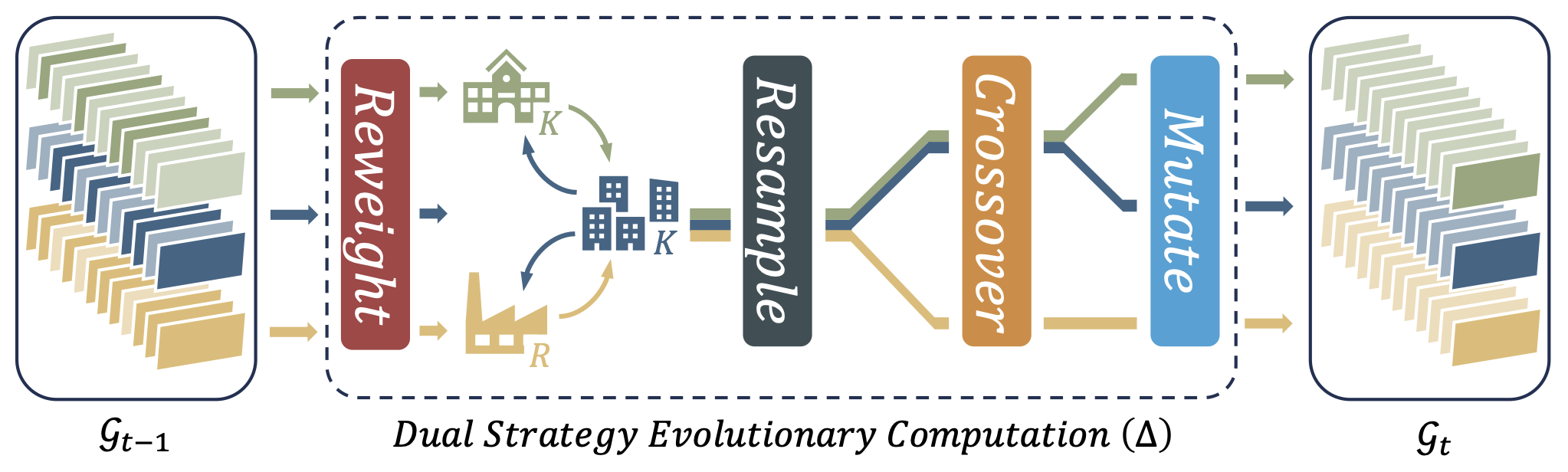
Fig. 2 illustrates the workflow of an epoch in DSE-SMC. As discussed in section 2.3, DSE-SMC is an iterative framework: at epoch , it maintains a set of weighted samples; and for , it runs five steps to evolve from to , namely reweight, migrate, resample, crossover, and migrate. Algorithm 1 shows the pseudocode of our DSE-SMC framework with more algorithmic details. The algorithm takes a black-box probabilistic semantics as its input, where stands for a probabilistic program and is its input space. In the setting of worst-case analysis, is usually an ordinary program with a resource-accumulation semantics and we simply define . Our approach is dual-strategy, meaning that we segregate candidate samples into two groups, one for applying -strategy, the other for -strategy. Different strategies mean that we apply different crossover and mutation operations, as we will discuss later in this section. Notationally, we write for the th sample during the th epoch, as well as and for its group assignment and weight (or fitness score), respectively. We then write , , and to be , , and , respectively, where is the number of samples during the th epoch.
We then discuss the five steps in an epoch of DSE-SMC one-by-one.
Reweight
This step is trivial: we simply use to compute the weight of each sample.
Migrate
This step is introduced by the dual-strategy approach. As discussed in section 2.3, we take inspiration from reproduction strategies of organisms (Andrews and Harris, 1986): the -strategy works in crowded environments and centers all the resources on a limited number of offspring, hoping to generate high-quality offspring, whereas the -strategy works in uncrowded environments and produces a considerable number of offspring, hoping to increase diversity. In terms of optimization and computational resources, we realize the -strategy as exploitation, generating a few new samples and trying to reach local optima around the current samples; whereas we realize the -strategy as exploration, generating a lots of diverse new samples and trying to reach a high variance in terms of their fitness scores. In our implementation, we further split the group into an extreme- group and a mild- group. The purpose of setting a-mild group is just for controlling the total number of population; it uses essentially the same strategy as that of the extreme- group, and is only treated differently during migration.
DSE-SMC allows a random migration routine Migrate to update group assignments based on the current assignments and weights of the samples. In our implementation, the migration takes place freely between the extreme- group and the mild- group, but in a restricted manner between the extreme- group and the group. The main idea is to build a nature-inspired routine of attracting candidates from the group to the group, as well as eliminating those candidates with relatively small weights from the group. Note that the motivation that drives candidates from the group to the group is greatly influenced by the difference in average weights. In our implementation, we use to determine the migration rate from to . After we determine the migration rate, the fitness scores of the candidates are view as criteria in deciding their weights in a Roulette wheel selection process, which means that candidates with higher scores have higher chances to migrate. The migration rate from to is simply a fixed rate, just for discarding candidates with relatively small weights from the group.
Resample
This step is basically the same as the adaptive resampling step of resample-move SMC. The difference is that DSE-SMC does not guarantee that the population size is a constant; instead, the population size at the th epoch is denoted as . This is because crossover and mutation operations can generate a different number of new samples. Therefore, we also perform a resampling step when the current sample size is greater than a pre-specified threshold .
After the resampling step, our algorithm again separates the current population into two, denoted by and , for the group and the group, respectively. For each group, the algorithm then proceeds with the rejuvenating step, which first performs crossover-based MCMC transitions and then repeatedly performs mutation-based MCMC transitions until some stop criterion is met. Note that crossover, mutation, and stop criterion are all group-specific.
To recast genetic operations in our DSE-SMC framework, we follow the idea of population-based MCMC (Jasra et al., 2007) and evolutionary MCMC (Drugan and Thierens, 2003) to integrate Metropolis-Hastings algorithms with genetic proposal distributions. The idea has been reviewed in section 2.3; thus, in the rest of this section, we present the genetic operations used in our implementation.
Crossover
This step is basically to carry out random uniform crossover within groups. Parent pairs are selected from the same group randomly, and for each pair, we sample a string, where the proportion of ones corresponds to crossover rate, deciding whether a part of the new offspring should be taken from one of the parents.
Mutate
This step is mainly achieved utilizing bit flip, one of the standard mutation techniques. Mutation is performed on every candidate as a bounded exploration mechanism within a small neighborhood of that candidate. Every bit of the candidate is considered separately: with some probability, the bit gets flipped. After all bits have been decided, one mutated candidate is produced.
The setup of stopping criteria for and groups are slightly more sophisticated. To implement the dual strategy, we set different stopping criteria for different groups. For the group, the computational resource is sufficient enough for carrying out kilos of attempts and severe competition. Therefore, the criterion is set to be achieving better fitness scores than surrounding candidates that are slightly different from the one being mutated. On the other hand, for the group, the computational resource is scarce, and only capable of carrying out dozens of attempts. Thus, the criterion is set to be having higher mutation potential, which, in our implementation, means that the standard deviation of the fitness scores of surrounding candidates should be as high as possible.
Implementation
We implemented a prototype of DSE-SMC in Java, which consists of about 3,100 lines of code. We have not yet implemented a instrumentation routine, so currently we assume the program-to-be-analyzed is implemented as a Java class with an entry method and the program includes explicit tick statements to indicate resource usages (like the example in Fig. 1(a)). In some of the evaluation subjects, we actually utilized AFL (Zalewski, 2023) to carry out instrumentation. The source code of our prototype and the programs used in our evaluation are included in the submitted replication package.
4. Experimental Evaluation
In this section, we present an experimental evaluation of our implementation of DSE-SMC, in the hope of answering the following research questions.
-
•
RQ1: How well does DSE-SMC perform in comparison with existing black-box worst-case-analysis tools?
-
•
RQ2: Does the DSE-SMC’s MCMC-based rejuvenation outperform a locally-optimal variant of DSE-SMC?
4.1. Experimental Setup
To present a versatile evaluation of how DSE-SMC may have an impact on both the basic algorithms and complex industrial applications, we select eight evaluation subjects, summarized in Tab. 1. Some of the subjects are adapted from recent work on WCA, e.g., SlowFuzz (Petsios et al., 2017) and Mayhem (Cha et al., 2012). The subjects on the left column of Tab. 1 are basic algorithms that may serve to create a general sense of how DSE-SMC works in terms of input mutation and worst-case navigating. On the other hand, the subjects on the right column of Tab. 1 are believed to be of great importance to the software industry. Note that we use different resource metrics for different subjects. The subjects on the left column are to be evaluated by observing the steps that the algorithm takes to halt, whereas those on the right column via counting the jumps that the application takes to complete the task.
| ID | Subject | ID | Subject |
|---|---|---|---|
| 1 | Generate ordered pairs | 5 | RegExa |
| 2 | Insertion sort | 6 | Hash table |
| 3 | Quicksort | 7 | Compression |
| 4 | Tree sort | 8 | Smart contract |
| awith fixed regex expression. | |||
For all evaluation subjects, we ran four WCA tools: (1) Kelinci, (2) KelinciWCA, (3) Locally-optimal DSE-SMC, and (4) DSE-SMC. Kelinci provides an interface for running AFL (Zalewski, 2023) on Java programs (Kersten et al., 2017) and KelinciWCA extends Kelinci to prioritize execution paths with high resource consumption (Noller et al., 2018). We include in the comparison a locally-optimal variant of DSE-SMC, which replaces the MCMC-based rejuvenation step with a local search that only keeps a locally optimal new candidate. It is of vital importance to control the basic setup and the initial value as they can greatly affect the performance of each tool. Therefore, we use the same meaningless inputs and default parameters to setup our evaluation. We ran each tool on each subject for at most 100 epochs or 100 minutes, which we will elaborate in the setup of each evaluation subject.
Note that there are also recently proposed WCA tools, such as SlowFuzz (Petsios et al., 2017), that execute evolutionary WCA on binary codes. Because we setup our experiments on Java programs, we cannot compare DSE-SMC with them directly. Nevertheless, we find that Badger (Noller et al., 2018), a WCA tool that integrates fuzzing and symbolic execution, can serve as an indirect indicator for comparison. The authors of Badger claim that black-box fuzzing-based WCA tools like SlowFuzz are in spirit similar to KelinciWCA. Thus, our comparison with KelinciWCA should reflect how our DSE-SMC framework performs against SlowFuzz, etc. A more systematic comparison (e.g., reimplement SlowFuzz and Mayhem’s algorithms for analyzing Java programs) is left for future work.
All of our experiments were conducted on an x86-64 architecture, Intel Core i7-1365UE 4.9GHz Linux machine with 32 GB of memory. We used OpenJDK 1.9.0_132 and configured the Java VM to use at most 10 GB of memory.
4.2. Ordering
We embark on the very basic algorithm in computer science: comparing and ordering. The first experiment we conducted is on pairing procedures to collect pairs that satisfy specific conditions, or in the case of our setup, ordered adjacent pairs. Because the structure of the experiment is relatively less sophisticated, the result shows that our approach behaves significantly better than Kelinci and KelinciWCA.
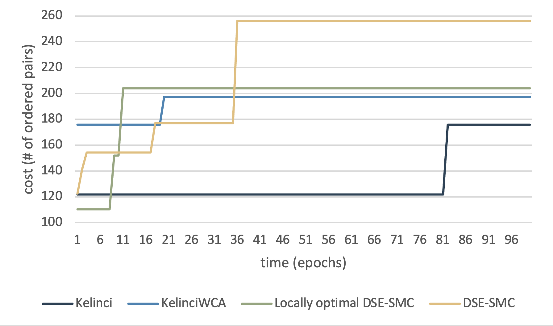
Fig. 3 displays the result of generating ordered pairs on a given array, where is the length of the array. The exact maximum score in this task is , and DSE-SMC reaches worst-case performance in less than minutes. All of the evaluated tools reach scores no less than of the maximum score in epochs, and converge no greater than epochs.
4.3. Sorting
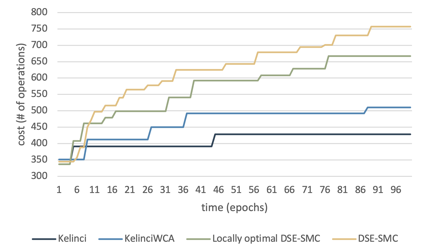
We then evaluate how our framework reacts to textbook algorithms, which are also evaluated in other WCA tools. In this section, we consider three sorting algorithms. Insertion sort and quicksort vary in terms of time complexity and the number of jumps. Both of them are easy to implement and execute, yet the worst-case behavior may be significantly influenced by the size of the input. In line with the execution time limit, we conducted our experiment on an implementation of insertion sort under input size of and present our results in Fig. 4, where is the input size.
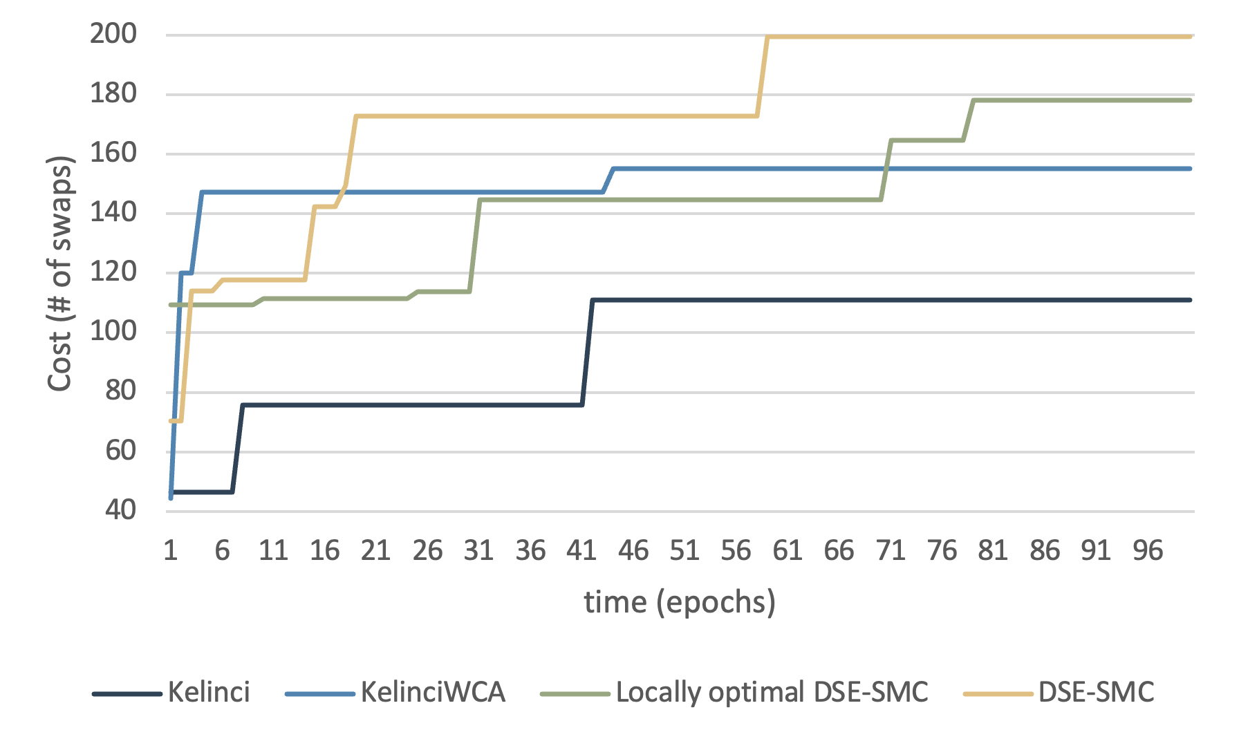
The exact maximum score (i.e., the number of swaps) possible for insertion sort is . From the result shown in Fig. 4, we observe that the score increases continuously when running DSE-SMC. The use of genetic mutation and crossover generally reduce the running time consumed to converge by epochs. Last but not least, KelinciWCA utilizes the customized cost function and indeed performed better at first epochs, yet failed to mutate towards larger scores in a restricted time frame.
The results for quicksort are shown in Fig. 5. After executing for 100 epochs, DSE-SMC behaves better than Kelinci by . On the other hand, we also notice that DSE-SMC behaves quite unsteady on the quicksort task. The minor drawback may be explained by the probabilistic mutation process and its inherited randomness. Overall, or in a slightly longer period, DSE-SMC converges 8 times quicker than KelinciWCA.
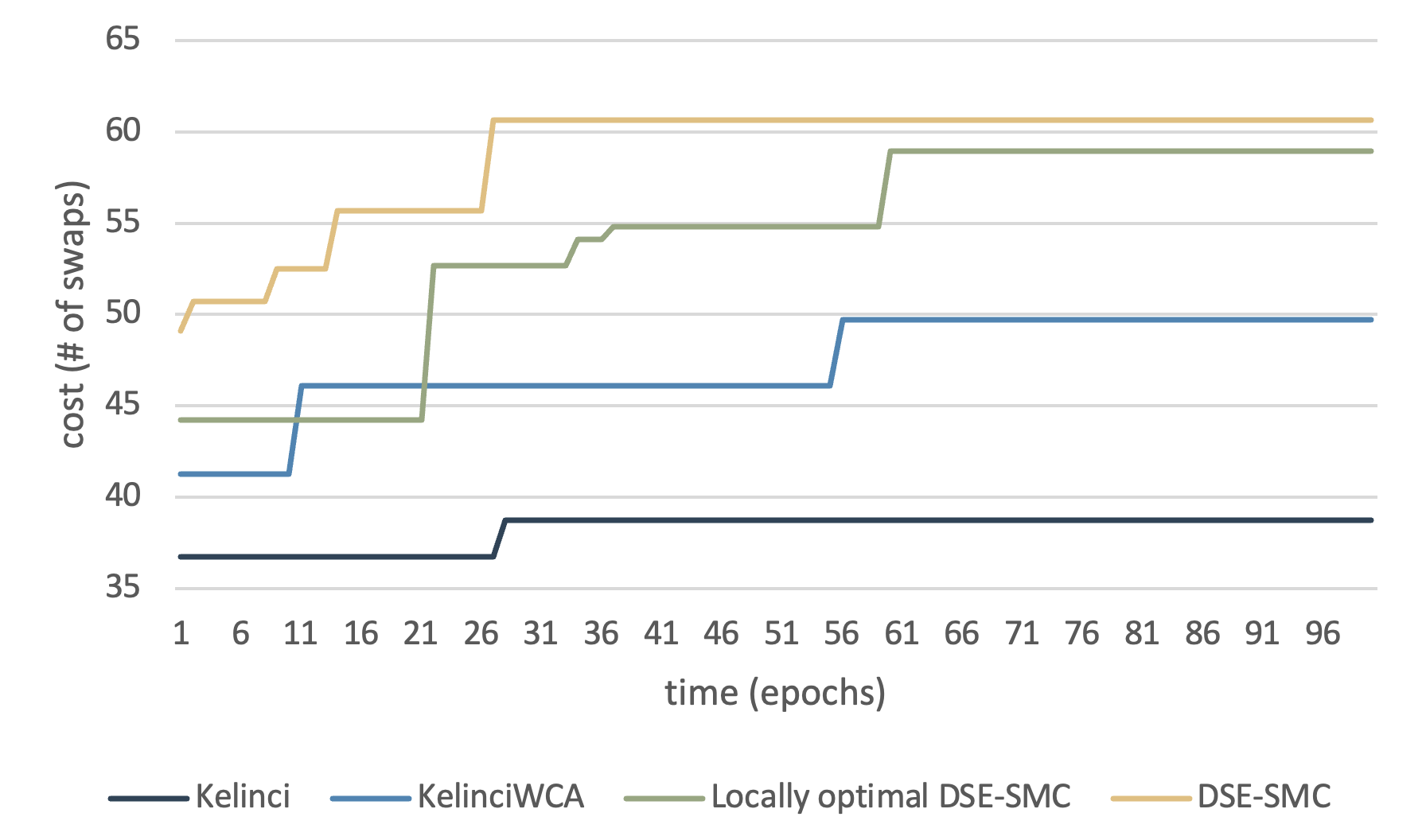
The last sorting task we investigated is the process we called tree sort. It is used to demonstrate the performance of DSE-SMC on subjects that use complex data structures. In this subject, we implemented a red-black tree for inserting integers and set the resource metric to be the number of red-black tree operations. The tendency and convergence rate of DSE-SMC in comparison with other tools are obvious, as shown in Fig. 6: our tool achieved a significantly faster speed to discover worst-case inputs.
4.4. RegEx
To secure an idea of what our approach behaves in extreme cases which are generally considered important in detecting vulnerabilities, we conduct the experiment on regular expression Denial-of-Service (ReDos) vulnerabilities.
In accordance with prior work (e.g., (Noller et al., 2018)), we used the java.util.regex JDK package.
It is generally used for vulnerability revelation and not exactly suitable to test worst-case generating.
Yet the results may be of help to understand the cons of applying black-box techniques to those type of problems.
In this experiment, we fixed the regular expression and attempted to mutate the text for worst-case inputs.
The ultimate goal for this example is that the WCA tools generate a password that matches the regular expression ((?=.*\d)(?=.*[a - z])(?=.*[A - Z])(?=.*[@#$%]).{6, 20}).
Fig. 7 shows the experimental result. DSE-SMC behaved slightly worse than the locally-optimal variant of DSE-SMC, and got caught up by Kelinci at approximately minutes. The results can be interpreted as lack of detailed domain knowledge with regard to the program structure. White- or grey-box tools in general have components for condition analysis and dynamic instrumentation. While black-box tools (like ours) execute faster in a single epoch, there is a choice between sacrificing computational speed and extracted information in one epoch when it comes to structural information within the program. Interestingly, the performance of DSE-SMC varies greatly across different runs. Inherited from probabilistic computation, DSE-SMC displays specific characters of randomness.
4.5. Hash Table
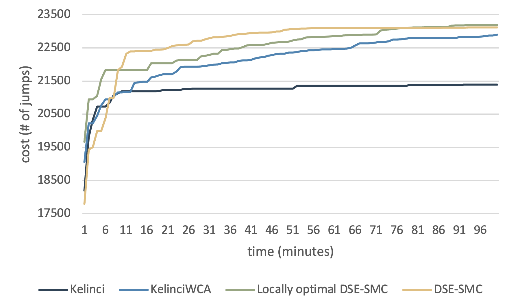
The hash-table subject is also implemented with considerations similar to RegEx. We modified the input part of the hash-table algorithm in accordance with prior work. Based on the outcome, we observe that there are several noises that seem to show that our tool generates worst-case inputs significantly better. By the one-hour time limit, our full version of DSE-SMC has already generated input cases that can trigger more than jumps, while KelinciWCA and locally-optimal DSE-SMC got stuck at near jumps. That displays a significant advancement, as shown in Fig. 8.
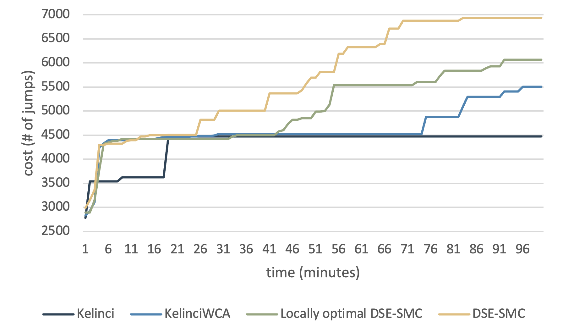
Another observation is that our tool continues to make progress at the end of the evaluation process. This indicates that probabilistic implementation of the genetic operations possess higher potential of exploration and the dual-strategy approach does make sense with regard to biological investigation. In addition, unlike the previous subjects of experiments, the performance of our tool on this subject is relatively stable in comparison, indicating the particular posterior distribution is a relatively smooth territory.
4.6. Compression
A normal application of WCA is to analyze the performance of compression algorithms.
Compression algorithms are a hot topic in both the industry and the academia.
We used the org.apache.commons.compress JDK package to conduct our experiment.
The subject to be tested is the performance of compression algorithms on bytes of input data.
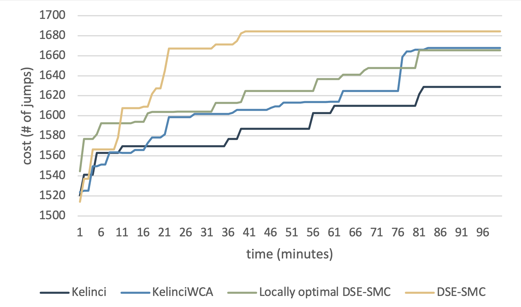
Fig. 9 shows the experimental result. Despite the difference in initial performances, DSE-SMC reaches 1680 jumps at least 3 times faster than KelinciWCA, and the locally optimal DSE-SMC makes steady progress and performs slightly better than KelinciWCA. The locally-optimal variant of DSE-SMC generated initial inputs that already lead to relatively high resource costs, yet slowed down quickly and got caught up by KelinciWCA at 23 minutes. DSE-SMC, on the other hand, reveals great potential in exploration that it boosts quickly, for example, in the th and th minutes. This can be explained by the fact that we use genetic mutation loops, which adds more steps relevant to exploration. It is also worth mentioning that we observe a slowdown after the boosts, indicating that our framework probably reaches a local optimum and bit-level mutation does no longer lead to better exploration. Although DSE-SMC continues to make progress after 100 minutes, at that point, one should decrease the rate of annealing the population and the migration rate of candidates applying the -strategy to address the issue and look for stabler balance between exploration and exploitation.
4.7. Smart Contract
One of the most interesting potentials for worst-case estimation is the potential of gas fuzzing in modern blockchains. Generally, the gas is a deterministic indicator that determines the cost of a smart contract and the resource consumption in executing it. We setup the environment in a simple smart contract in a Java-based form. Details can be found in the replication package.
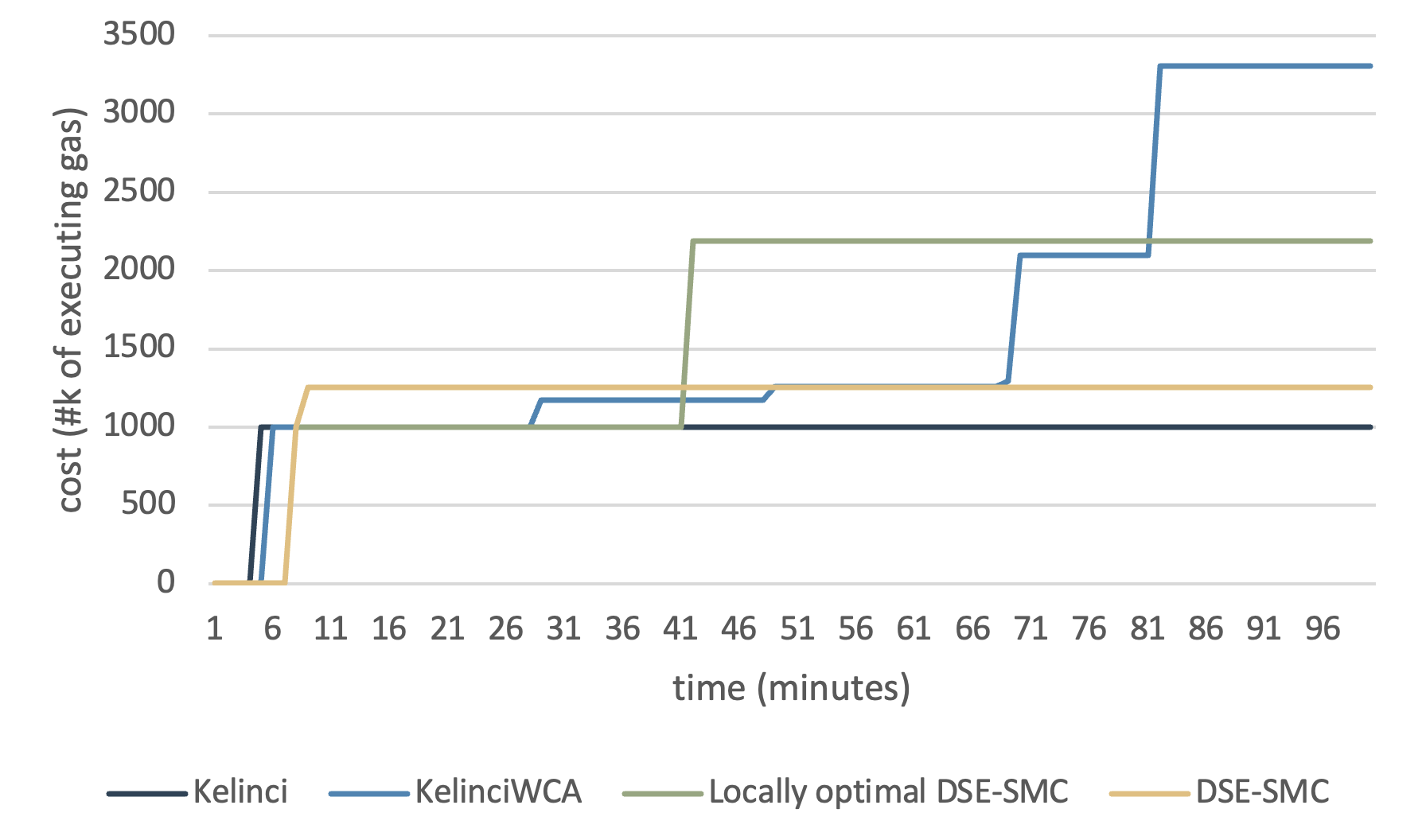
Results for this subject are displayed in Fig. 10. As the cost is user-defined, we have to manually set the cost in order to feed Kelinci and KelinciWCA. We conducted the experiment for multiple times and got results with huge variation. Our DSE-SMC tool does not perform as good as one would expect. An observation from the smart-contract experiment is that DSE-SMC generally got stuck at 10 minutes and behaved worse than KelinciWCA. In addition, time consumed in one epoch is relatively greater than other tools due to the implementation of different strategies and relatively complex rejuvenation routines. Note that the smart-contract experiment we conduct is based on its gas consumption, whose calculation mainly replies on memory allocation and pointers’ inner relationships. Without inner relationship or fine-grained program analysis, black-box based tools are easy to miss target branches which consume a lot of gas, and therefore, fail to observe overall worse-case gas-usage behavior. It would be interesting future research to integrate our black-box technique with white- or grey-box approaches that can provide more application-specific information.
4.8. Threats to Validity
Internal Validity
The main threat to internal validity is the theoretical structure of DSE-SMC. We have cross validate the revise the theoretical process to ensure the solidity as best as we can. Another threat worth mentioning is the choice of parameters that are integrated in our framework. As it is computational costly, and therefore, impractical for testers to manually set those parameters to suit each subjects, we did pre-experiments beforehand on subject 2 to mitigate the effects. Yet the choice can still be customized, and consequently display results significantly different from each other to concernable extent. Also, experiments are conducted on server that are not often reliable in terms of execution speed and resource consumption. In future practice, we will look into methods of parallelizing the dual strategy implementation. Theoretical speaking, we could expect a speedup of 1.5x, which is an outstanding improvement in efficiency.
External Validity
The main threat to external validity is the direction in which we pick the subjects and conduct the experiments. These subjects are not generalized or regulated, and therefore may not be suitable for tool comparing to some related work. To mitigate this concern, we select many of our benchmarks that are in line with the existing work similar to ours. In addition, the pile insertion part for basic performance monitoring of our framework is implemented using external tools, which can potentially be incorrect and threaten our validity.
5. Related Work
Worst-Case Analysis
Most related to our work are techniques for conducting worst-case analysis by generating worst-case inputs. In this paper, we focus on black-box approaches, which are agnostic of application-specific or implementation-specific domain knowledge. Most recent work along this line includes KelinciWCA (Noller et al., 2018) and SlowFuzz (Petsios et al., 2017). We have presented an empirical comparison of our DSE-SMC framework to those techniques in section 4. The major difference is that DSE-SMC is based on an WCA-is-MAP observation and a novel dual-strategy evolutionary sequential-Monte-Carlo algorithm.
Another popular line of work for worst-case analysis is based on symbolic execution. Those techniques need to look into the concrete structures of analyzed programs, so they are fundamentally different from our focus in this paper. WISE (Burnim et al., 2009) explores all program paths to find worst-case ones on small inputs, and then uses those paths to derive a heuristic to generate larger worst-case inputs. SPF-WCA (Luckow et al., 2017) introduces path policies to guide the search of symbolic execution. Wang and Hoffmann (2019) proposes a type-guided worst-case input generation that utilizes resource-aware type derivation (Hoffmann et al., 2017) to prune the search space of symbolic execution. Badger (Noller et al., 2018) combines symbolic execution with fuzzing techniques to generate high-resource-usage inputs to avoid exhaustive exploration of program paths. Our future research may investigate how to incorporate symbolic execution in DSE-SMC.
Fuzzing
Fuzzing receives more and more attraction now that the scale of codes increases significantly (McNally et al., 2012). It has the following advantages over other testing techniques: (1) no requirements for source code of the analyzed program, (2) more faster in comparison to human testers, (3) relatively less expensive, and (4) more generic and portable. In our work, DSE-SMC can be seen as a fuzzer that targets the generation of worst-case inputs for Java programs. The tool is conceptually similar to general black-box fuzzers including AFL (Zalewski, 2023) and LibFuzzer (LLVM Project, 2023). Our innovation is the integration of evolutionary fuzzing into the sequential-Monte-Carlo framework and the development of the dual-strategy approach.
Similar to WCA, recent fuzzers also possesses great potential especially with the help of symbolic-execution engines. To name a few, Mayhem (Cha et al., 2012), a symbolic execution engine, combined with the Murphy fuzzer, won the 2016 DARPA Cyber Grand Challenge. EvoSuite (Galeotti et al., 2013) is a test-case generation tool with dynamic symbolic execution for Java.
Sequential Monte Carlo
The key sequencial structure of DSE-SMC is based on sequential Monte Carlo (SMC). There are many developed algorithms that can be integrated in DSE-SMC as a sequence building techniques, including SMC samplers (Del Moral et al., 2006), bootstrap SMC filters (Candy, 2007), resample-move SMC (Gilks and Berzuini, 2001; Chopin, 2002), etc. Chen et al. (2000) summarizes some commonly used cases of SMC. Despite some concerns on degeneracy (Candy, 2007) and introducing non-independent data, bridge sampling (Bennett, 1976) alleviates the concerns of cases with high-dimensional posterior (e.g. (Frühwirth-Schnatter, 2004)). Generally, SMC serves as a crucial part in dynamic bayesian models, for example, MCMC rejuvenation (Gilks and Berzuini, 2001). SMCP3 (Lew et al., 2023) has broaden the scope of SMC to incorporate probabilistic auxiliary variables during inference. Besides, if the prior and posterior distributions have a similar shape or strong overlap, a naive Monte Carlo estimator could also be a satisfactory choice. Starting from this work, we hope to systematically investigate SMC-based fuzzing for software testing.
Nature-Inspired Algorithms
The population-based meta-heuristics approach we adapt in this paper is to address the concern that single-solution-based meta-heuristics may get stuck in local optima (Kumar and Kumar, 2017). The process connecting the sequential structure within DSE-SMC is the originated from genetic algorithms (Goldberg, 1989), and inspired by swarm intelligence algorithms like particle swarm optimization (PSO) (Kennedy and Eberhart, 1995) ant colony optimization (ACO) (Dorigo et al., 2008). Intuitively and naturally, nature-inspired algorithms have been put forward to imitate, simulate and better approximate the natural process of evolution in complicated environment than classic algorithms. It would be interesting future research to incorporate more nature-inspired algorithms into sequential Monte Carlo.
6. Conclusion
We have presented Dual-Strategy Evolutionary Sequential Monte-Carlo (DSE-SMC) framework for black-box worst-case-analysis fuzzing. The framework is built upon a key observation discussed in this paper: worst-case analysis (WCA) is isomorphic to maximum-a-posteriori (MAP) estimation in the context of Bayesian inference. DSE-SMC incorporates resample-move SMC, evolutionary MCMC, nature-inspired - and -strategies, and fuzz testing to provide a generic, adaptive, and sound framework for worst-case analysis. We implemented a prototype of DSE-SMC and evaluated its effectiveness on several subject programs.
In the future, we plan to dig further into the correspondence between WCA and MAP. So far we have not used the prior distributions that are common in probabilistic models. In the context of Bayesian inference, prior distributions are usually used to encode domain information, and thus to guide inference algorithms. Is it possible to cast white-box analysis results (e.g., program analysis, type derivation, and symbolic execution) as prior distributions to provide insights for WCA? Another research direction is to transfer other Bayesian-inference algorithms to carry out WCA. For example, recent advances in variational inference render it as a promising technique for approximating posterior distributions. It would be interesting to see if it is applicable to WCA.
References
- (1)
- Andrews and Harris (1986) John H. Andrews and Robin F. Harris. 1986. - and -Selection and Microbial Ecology. In Advances in Microbial Ecology. Springer, Boston, MA. https://doi.org/10.1007/978-1-4757-0611-6_3
- Barthe et al. (2020) Gilles Barthe, Joost-Pieter Katoen, and Alexandra Silva (Eds.). 2020. Foundations of Probabilistic Programming. Cambridge University Press. https://doi.org/10.1017/9781108770750
- Bennett (1976) Charles H Bennett. 1976. Efficient estimation of free energy differences from Monte Carlo data. J. Comput. Phys. 22 (October 1976), 245–268. Issue 2. https://doi.org/10.1016/0021-9991(76)90078-4
- Bingham et al. (2018) Eli Bingham, Jonathan P. Chen, Martin Jankowiak, Fritz Obermeyer, Neeraj Pradhan, Theofanis Karaletsos, Rishabh Singh, Paul Szerlip, Paul Horsfall, and Noah D. Goodman. 2018. Pyro: Deep Universal Probabilistic Programming. J. Machine Learning Research 20 (January 2018). Issue 1. https://dl.acm.org/doi/10.5555/3322706.3322734
- Borgström et al. (2016) Johannes Borgström, Ugo Dal Lago, Andrew D. Gordon, and Marcin Szymczak. 2016. A Lambda-Calculus Foundation for Universal Probabilistic Programming. In Int. Conf. on Functional Programming (ICFP’16). https://doi.org/10.1145/2951913.2951942
- Burnim et al. (2009) Jacob Burnim, Sudeep Juvekar, and Koushik Sen. 2009. WISE: Automated Test Generation for Worst-Case Complexity. In Int. Conf. on Softw. Eng. (ICSE’09). 463–473. https://doi.org/10.1109/ICSE.2009.5070545
- Candy (2007) James V. Candy. 2007. Bootstrap Particle Filtering. Signal Processing Magazine 24 (July 2007), 73–85. Issue 4. https://doi.org/10.1109/MSP.2007.4286566
- Carpenter et al. (2017) Bob Carpenter, Andrew Gelman, Matthew D. Hoffman, Daniel Lee, Ben Goodrich, Michael Betancourt, Marcus Brubaker, Jiqiang Guo, Peter Li, and Allen Riddell. 2017. Stan: A Probabilistic Programming Language. J. Statistical Softw. 76 (January 2017). Issue 1. https://doi.org/10.18637/jss.v076.i01
- Cha et al. (2012) Sang Kil Cha, Thanassis Avgerinos, Alexandre Rebert, and David Brumley. 2012. Unleashing Mayhem on Binary Code. In Symposium on Security and Privacy (SP’12). 380–394. https://doi.org/10.1109/SP.2012.31
- Chen et al. (2000) Ming-Hui Chen, Qi-Man Shao, and Joseph G. Ibrahim. 2000. Monte Carlo Methods in Bayesian Computation. Springer New York, NY. https://doi.org/10.1007/978-1-4612-1276-8
- Chopin (2002) Nicolas Chopin. 2002. A sequential particle filter method for static models. Biometrika 89 (August 2002), 539–552. Issue 3. https://doi.org/10.1093/biomet/89.3.539
- Cusumano-Towner et al. (2019) Marco F. Cusumano-Towner, Feras A. Saad, Alexander K. Lew, and Vikash K. Mansinghka. 2019. Gen: A General-Purpose Probabilistic Programming System with Programmable Inference. In Prog. Lang. Design and Impl. (PLDI’19). https://doi.org/10.1145/3314221.3314642
- Del Moral et al. (2006) Pierre Del Moral, Arnaud Doucet, and Ajay Jasra. 2006. Sequential Monte Carlo Samplers. J. Royal Statistical Society 68 (January 2006). Issue 3. https://www.jstor.org/stable/3879283
- Del Moral et al. (2007) Pierre Del Moral, Arnaud Doucet, and Ajay Jasra. 2007. Sequential Monte Carlo for Bayesian Computation. Bayesian Statistics 8 (2007).
- Del Moral et al. (2001) Pierre Del Moral, L. Kallel, and J. Rowe. 2001. Modeling genetic algorithms with interacting particle systems. Revista De Matemática: Teoría Y Aplicaciones 8 (2001), 19–77. Issue 2. https://doi.org/10.15517/rmta.v8i2.201
- Dorigo et al. (2008) Marco Dorigo, Mauro Birattari, Christian Blum, Maurice Clerc, Thomas Stützle, and Alan F. T. Winfield (Eds.). 2008. Ant Colony Optimization and Swarm Intelligence. Springer Berlin, Heidelberg. https://doi.org/10.1007/978-3-540-87527-7
- Drugan and Thierens (2003) Mădălina M. Drugan and Dirk Thierens. 2003. Evolutionary Markov Chain Monte Carlo. In International Conference on Artificial Evolution (EA’03). 63–76. https://doi.org/10.1007/978-3-540-24621-3_6
- Dufays (2016) Arnaud Dufays. 2016. Evolutionary Sequential Monte Carlo Samplers for Change-Point Models. Econometrics 4 (March 2016). Issue 1. https://doi.org/10.3390/econometrics4010012
- Frühwirth-Schnatter (2004) Sylvia Frühwirth-Schnatter. 2004. Estimating marginal likelihoods for mixture and Markov switching models using bridge sampling techniques. The Econometrics Journal 7 (June 2004), 143–167. Issue 1. https://doi.org/10.1111/j.1368-423X.2004.00125.x
- Galeotti et al. (2013) Juan Pablo Galeotti, Gordon Fraser, and Andrea Arcuri. 2013. Improving search-based test suite generation with dynamic symbolic execution. In International Symposium on Software Reliability Engineering (ISSRE’13). 360–369. https://doi.org/10.1109/ISSRE.2013.6698889
- Gelman et al. (2013) Andrew Gelman, John B. Carlin, Hal S. Stern, David B. Dunson, Aki Vehtari, and Donald B. Rubin. 2013. Bayesian Data Analysis. Chapman and Hall/CRC. https://doi.org/10.1201/b16018
- Ghahramani (2015) Zoubin Ghahramani. 2015. Probabilistic machine learning and artificial intelligence. Nature 521 (May 2015), 452–459. https://doi.org/10.1038/nature14541
- Gilks and Berzuini (2001) Walter R. Gilks and Carlo Berzuini. 2001. Following a Moving Target-Monte Carlo Inference for Dynamic Bayesian Models. Journal of the Royal Statistical Society 63 (2001), 127–146. Issue 1.
- Goldberg (1989) David E. Goldberg. 1989. Genetic Algorithms in Search, Optimization and Machine Learning. Addison-Wesley Longman Publishing Co., Inc.
- Goodman et al. (2008) Noah D. Goodman, Vikash K. Mansinghka, Daniel Roy, Keith A. Bonawitz, and Joshua B. Tenenbaum. 2008. Church: A language for generative models. In Uncertainty in Artificial Intelligence (UAI’08). https://dl.acm.org/doi/10.5555/3023476.3023503
- Goodman and Stuhlmüller (2014) Noah D. Goodman and Andreas Stuhlmüller. 2014. The Design and Implementation of Probabilistic Programming Languages. Available on http://dippl.org.
- Griffiths et al. (2008) Thomas L. Griffiths, Charles Kemp, and Joshua B. Tenenbaum. 2008. Bayesian Models of Cognition. In The Cambridge Handbook of Computational Psychology. Cambridge University Press. https://doi.org/10.1017/CBO9780511816772.006
- Gu et al. (2015) Shixiang Gu, Zoubin Ghahramani, and Richard E. Turner. 2015. Neural Adaptive Sequential Monte Carlo. In Neural Info. Processing Syst. (NIPS’15). https://dl.acm.org/doi/10.5555/2969442.2969533
- Hoffmann et al. (2017) Jan Hoffmann, Ankush Das, and Shu-Chun Weng. 2017. Towards Automatic Resource Bound Analysis for OCaml. In Princ. of Prog. Lang. (POPL’17). 359–373. https://doi.org/10.1145/3009837.3009842
- Jasra et al. (2007) Ajay Jasra, David A. Stephens, and Christopher C. Holmes. 2007. Population-Based Reversible Jump Markov Chain Monte Carlo. Biometrika 94 (December 2007), 787–807. Issue 4.
- Kennedy and Eberhart (1995) James Kennedy and Russell C. Eberhart. 1995. Particle swarm optimization. In International Conference on Neural Networks (ICNN’95). 1942–1948. https://doi.org/10.1109/ICNN.1995.488968
- Kersten et al. (2017) Rody Kersten, Kasper Luckow, and Corina S. Păsăreanu. 2017. POSTER: AFL-based Fuzzing for Java with Kelinci. In Computer and Communications Security (CCS’17). 2511–2513. https://doi.org/10.1145/3133956.3138820
- Kozen (1981) Dexter Kozen. 1981. Semantics of Probabilistic Programs. J. Comput. Syst. Sci. 22 (June 1981). Issue 3. https://doi.org/10.1016/0022-0000(81)90036-2
- Kumar and Kumar (2017) Vijay Kumar and Dinesh Kumar. 2017. An astrophysics-inspired Grey wolf algorithm for numerical optimization and its application to engineering design problems. Advances in Engineering Software 112 (October 2017), 231–254. https://doi.org/10.1016/j.advengsoft.2017.05.008
- Kwok et al. (2005) Ngaiming Kwok, Gu Fang, and Weizhen Zhou. 2005. Evolutionary particle filter: re-sampling from the genetic algorithm perspective. In International Conference on Intelligent Robots and Systems (IROS’05). 2935–2940. https://doi.org/10.1109/IROS.2005.1545119
- Lew et al. (2023) Alexander K. Lew, George Matheos, Tan Zhi-Xuan, Matin Ghavamizadeh, Nishad Gothoskar, Stuart Russell, and Vikash K. Mansinghka. 2023. SMCP3: Sequential Monte Carlo with Probabilistic Program Proposals. In Artificial Intelligence and Statistics (AISTATS’23). 7061–7088.
- Liang and Wong (2000) Faming Liang and Wing Hung Wong. 2000. Evolutionary Monte Carlo: Applications to Model Sampling and Change Point Problem. Statistica Sinica 10 (April 2000), 317–342. Issue 2.
- LLVM Project (2023) LLVM Project. 2023. libFuzzer – a library for coverage-guided fuzz testing. Available on https://llvm.org/docs/LibFuzzer.html.
- Luckow et al. (2017) Kasper Luckow, Rody Kersten, and Corina S. Păsăreanu. 2017. Symbolic Complexity Analysis Using Context-Preserving Histories. In Int. Conf. on Softw. Testing, Verif. and Validation (ICST’17). 58–68. https://doi.org/10.1109/ICST.2017.13
- McNally et al. (2012) Richard McNally, Ken Yiu, Duncan Grove, and Damien Gerhardy. 2012. Fuzzing: The State of the Art. Available on https://apps.dtic.mil/sti/citations/ADA558209.
- Noller et al. (2018) Yannic Noller, Rody Kersten, and Corina S. Păsăreanu. 2018. Badger: Complexity Analysis with Fuzzing and Symbolic Execution. In Int. Symp. on Softw. Testing and Analysis (ISSTA’18). 322–332. https://doi.org/10.1145/3213846.3213868
- Petsios et al. (2017) Theofilos Petsios, Jason Zhao, Angelos D. Keromytis, and Suman Jana. 2017. SlowFuzz: Automated Domain-Independent Detection of Algorithmic Complexity Vulnerabilities. In Computer and Communications Security (CCS’17). 2155–2168. https://doi.org/10.1145/3133956.3134073
- Saad et al. (2023) Feras A. Saad, Brian Patton, Matthew D. Hoffman, Rif A. Saurous, and Vikash K. Mansinghka. 2023. Sequential Monte Carlo Learning for Time Series Structure Discovery. In International Conference on Machine Learning (ICML’23). 29473–29489.
- Thrun et al. (2005) Sebastian Thrun, Wolfram Burgard, and Dieter Fox. 2005. Probabilistic Robotics. MIT Press. https://dl.acm.org/doi/10.5555/1121596
- Wang and Hoffmann (2019) Di Wang and Jan Hoffmann. 2019. Type-guided worst-case input generation. Proceedings of the ACM on Programming Languages 3, 13 (January 2019), 13:1–13:30. Issue POPL. https://doi.org/10.1145/3290326
- Wigren et al. (2018) Anna Wigren, Lawrence M. Murray, and Fredrik Lindsten. 2018. Improving the particle filter in high dimensions using conjugate artificial process noise. In IFAC Symp. on System Identification (SYSID’18). https://doi.org/10.1016/j.ifacol.2018.09.207
- Zalewski (2023) Michal Zalewski. 2023. america fuzzy lop. Available on https://lcamtuf.coredump.cx/afl/.
- Zhu et al. (2018) Gaofeng Zhu, Xin Li, Jinzhu Ma, Yunquan Wang, Shaomin Liu, Chunlin Huang, Kun Zhang, and Xiaoli Hu. 2018. A new moving strategy for the sequential Monte Carlo approach in optimizing the hydrological model parameters. Advances in Water Resources 114 (April 2018), 164–179. https://doi.org/10.1016/j.advwatres.2018.02.007
- Zhu et al. (2022) Xiaogang Zhu, Sheng Wen, Seyit Camtepe, and Yang Xiang. 2022. Fuzzing: A Survey for Roadmap. Comput. Surveys 54, 230 (September 2022), 230:1–230:36. Issue 11s. https://doi.org/10.1145/3512345