Worst-Case Optimal Investment
in Incomplete Markets

Sascha Desmettre S. Desmettre, Institute of Financial Mathematics and Applied Number Theory, Johannes Kepler University (JKU) Linz, A-4040 Linz, Austria. sascha.desmettre@jku.at , Sebastian Merkel S. Merkel, School of Economics, University of Bristol, Priory Road Complex, Priory Road, Bristol BS8 1TU, United Kingdom. s.merkel@bristol.ac.uk , Annalena Mickel A. Mickel, Mathematical Institute and DFG Research Training Group 1953, University of Mannheim, B6, 26, D-68131 Mannheim, Germany and Alexander Steinicke A. Steinicke, Department of Mathematics and Information Technology, Montanuniversitaet Leoben, A-8700 Leoben, Austria. alexander.steinicke@unileoben.ac.at

(Date: December 16, 2024)

Abstract.

We study and solve the worst-case optimal portfolio problem as pioneered by Korn and Wilmott in [41] of an investor with logarithmic preferences facing the possibility of a market crash with stochastic market coefficients by enhancing the martingale approach developed by Seifried in [51]. With the help of backward stochastic differential equations (BSDEs), we are able to characterize the resulting indifference optimal strategies in a fairly general setting. We also deal with the question of existence of those indifference strategies for market models with an unbounded market price of risk. We therefore solve the corresponding BSDEs via solving their associated PDEs using a utility crash-exposure transformation. Our approach is subsequently demonstrated for Heston’s stochastic volatility model, Bates’ stochastic volatility model including jumps, and Kim-Omberg’s model for a stochastic excess return.
MSC (2010) codes: 49J55; 93E20; 91A15; 91B70
Key words: stochastic control, backward stochastic differential equations, worst-case approach, portfolio optimization, indifference strategies, incomplete markets

1. Introduction

An important aspect that is neglected in the pure Merton type portfolio optimization setting is the presence of so-called crash scenarios as first introduced by Hua and Wilmott [27] in discrete time. In this setting, parameters are subject to Knightian uncertainty in the sense of Knight [34], which consequently does not impose any distributional assumptions. In particular, in these worst-case optimization models, a financial crash is identified with an instantaneous jump in asset prices.

The literature strand on worst-case portfolio optimization possess by now a long history. In their seminal work [41], Korn and Wilmott have solved the worst-case scenario portfolio problem under the threat of a crash for logarithmic utility in continuous time. Their results have been extended in [36] by using the so-called indifference principle. Korn and Steffensen [40] then derive (classical) HJB systems for the worst-case portfolio problem. What all these works have in common from a conceptual point of view, is that the resulting worst-case optimal strategies are characterized by the requirement that the investor is indifferent between the worst crash happening immediately and no crash happening at all.

Based on a controller-vs-stopper game, Seifried introduced fundamental concepts for the worst-case portfolio optimization in [51], namely the indifference frontier, the indifference optimality principle and the change-of-measure device (see also [39]), in order to generalize the results to multi-asset frameworks and in particular discontinuous price dynamics. During the course of this paper, we will heavily rely on these methods and enhance them by allowing the market coefficients - in particular the volatility and the excess return - to be stochastic.

Further generalizations of the worst-case approach comprise, among others, proportional transaction costs, cf. [7], a random number of crashes, cf. [6], lifetime-consumption, cf. [17], a second layer of robustness, cf. [16], explicit solutions for the multi-asset framework, cf. [35], and more recently stress scenarios, cf. [38] and dynamic reinsurance, cf. [37].

From an abstract point of view, the worst-case approach shares common features with classical robust portfolio optimization, which typically focus on the financial markets’ parameters. For instance in [52], the market acts against the trader and chooses the worst possible market coefficients. Among others, another example is Schied, cf. [50], who considers a set of probability measures to maximize the robust utility of the terminal wealth. We refer to [22] for an overview on this literature. We however wish to stress that in the worst-case portfolio optimization problem, the jump times and the jump intensity are unknown, which renders the problem more delicate than standard portfolio optimization problems.

Another strand of literature, to which our work is related, is portfolio optimization with unhedegable risks, which typically comes along with incomplete markets. The seminal paper of Zariphopoulou [53] introduces the so-called martingale distortion, which is able to deal with stochastic volatility models in a very general factor model setting. Concerning Heston’s model, Kraft [42] finds explicit solutions for power utility using stochastic control methods. Martingale methods are then employed in [31] in an affine setting. Related works in that context include as well [47, 12, 46]. In a setting with stochastic excess return, Kim and Omberg [33] find optimal trading strategies for HARA utility functions. For a concise overview of asset allocation in the presence of jumps, both in the asset price and the volatility, we refer to [8] and the references therein. In the context of worst-case portfolio optimization, so far market coefficients are assumed to be constant - with the exception of Engler and Korn [21], who solve the worst-case optimization problem for a Vasicek short rate process.

In this work, we combine the strands of worst-case portfolio optimization and optimal investment with unhedgeable risks as follows:

•

We solve the worst-case optimal investment problem of an investor with logarithmic utility, facing both structural crashes and jump risk, in a setting that allows as well for stochastic market coefficients.
•

We enhance the concepts indifference frontier, the indifference optimality principle and the change-of-measure device to the case of stochastic market coefficients for logarithmic utility.
•

We characterize the resulting indifference strategies via the unique solutions of BSDEs, using the so-called utility crash exposure.
•

We exemplify and analyze the resulting indifference strategies for the Heston model, the Bates model and the Kim-Omberg model.

We also contribute to the general theory of backward stochastic differential equations, since the equation that emerges when describing indifference strategies, leads to a BSDE coefficient that does not satisfy a Lipschitz condition with deterministic constants. Rather, we are confronted with a stochastic Lipschitz constant that satisfies an exponential integrability condition. Additionally, the generator is exponentially integrable itself. In the setting without jumps, similar conditions, sufficient for existence and uniqueness, have e.g. been treated in [9], [19] and [45]. In the case including jumps, BSDEs with stochastic Lipschitz condition have been treated in [49, Chapter II]. However, the spaces for solutions used there are different than those in the standard theory with deterministic Lipschitz constants. Our results in this article still allow the use of the standard spaces. The approach we follow is based on an approximation argument building on the Lévy settings used e.g. in [44] and [43]. We obtain existence, uniqueness of a solution and a comparison theorem, necessary to guarantee the one-to-one relation between BSDEs and PDEs (see [3]). This relation between the deterministic and stochastic world needs several requirements, e.g. a local Lipschitz continuity in the initial value of the stochastic process that models the volatility of the asset price. To be applicable to the popular model choice of the CIR process, we extend the existing result from [13] to a wider parameter range.

The remainder of the paper is organized as follows: In Section 2 we define the financial market and and the worst-case optimization problem in incomplete markets. In Section 3 and and Section 4, we solve the worst-case portfolio optimization problem by disentangling the problem in the post-crash and pre-crash problem. Section 5 then develops the BSDE machinery which is needed for the characterization of indifference strategies when market coefficients are stochastic. Section 6 and Section 7 deal with the concrete examples, i.e. the Heston model, the Bates model and the Kim-Omberg model. Appendices A, B and C contain several proofs and auxiliary results.

2. Financial Market Model and Worst-Case Optimization Problem

Let $(\Omega,\mathcal{F},\mathbb{P})$ be a probability space carrying two independent Brownian motions $\hat{W},\tilde{W}$ and a Poisson random measure $\nu$ independent from $(\hat{W},\tilde{W})$ . $(\mathcal{F}_{t})_{t\in[0,T]}$ is the natural, augmented filtration for $\hat{W},\tilde{W}$ and $\nu$ satisfying the usual conditions. Note that for some $\rho\in[-1,1],W:=\rho\hat{W}+\sqrt{1-\rho^{2}}\tilde{W}$ is again a Brownian motion.

The financial market consists of a riskless money market account $B$ and a risky asset $S$ . In the absence of a crash, the dynamics of $B$ and $S$ are given by

	$\displaystyle dB_{t}$	$\displaystyle=B_{t}r_{t}dt\,,\quad$	$\displaystyle B_{0}=1\,,$
	$\displaystyle dS_{t}$	$\displaystyle=S_{t-}\left[(r_{t}+\lambda_{t})dt+\sigma_{t}\,dW_{t}-\int_{[0,l^{L}_{\max}]}l\nu(dt,dl)\right]\,,\quad$	$\displaystyle S_{0}=s\,,$

where $r$ , $\lambda$ and $\sigma>0$ are progressively measurable processes (w.r.t. the filtration $(\mathcal{F}_{t})_{t\in[0,T]}$ ) describing the dynamics of the market coefficients. Moreover, we denote the intensity measure of the Poisson random measure $\nu$ by $\vartheta$ and by $\tilde{\nu}$ we denote the according compensated Poisson random measure; we assume that $\vartheta$ is a Lévy measure with support in $[0,l^{L}_{\max}]$ and $\int_{[0,l^{L}_{\max}]}l\vartheta(dl)<\infty$ . In addition, we assume $l^{L}_{\max}<l^{WOC}$ , where $l^{WOC}\in(0,1)$ is the given size of the model’s worst-case substantial crash. If the model does not permit jumps (i.e. $\nu$ and $\vartheta$ do not appear), we call this setting purely Brownian model or model without jumps.

A particularly important choice of those parameters leads to the following version of the Bates model [5] and Heston model [26], respectively:

(1)	$\displaystyle dB_{t}$	$\displaystyle=B_{t}r_{t}dt\,,\quad$	$\displaystyle B_{0}=1\,,$
	$\displaystyle dS_{t}$	$\displaystyle=S_{t-}\left[(r_{t}+\lambda_{t})dt+\sqrt{z_{t}}\,dW_{t}-\int_{[0,l^{L}_{\max}]}l\nu(dt,dl)\right]\,,\quad$	$\displaystyle S_{0}=s\,,$
	$\displaystyle dz_{t}$	$\displaystyle=\kappa(\theta-z_{t})dt+\tilde{\varsigma}\sqrt{z_{t}}d\hat{W}_{t}\,,\quad$	$\displaystyle z_{0}=z\,,$

where $r$ is a progressively measurable interest rate process, $\lambda$ is a progressively measurable excess return process, $\theta>0$ the mean reversion level of the volatility, $\kappa>0$ the mean reversion speed of the volatility, $\tilde{\varsigma}>0$ the volatility of volatility and $\hat{W}$ is another Brownian motion with $\left<W,\hat{W}\right>_{t}=\rho t$ .

Alternatively, the Kim-Omberg model, cf. [33], is constituted by an analogous set of equations, where now $\lambda_{t}=z_{t}$ with constant $\sigma_{t}=\tilde{\sigma}\in(0,\infty)$ . We elaborate on the details in Section 6.

We face two types of crashes in our model. The number $l^{WOC}\in(0,1)$ describes the structural worst-case crash associated with a catastrophe. By $l$ we denote continuously occurring crashes of moderate size with $l\in(0,l^{L}_{\max}]$ , where $l^{L}_{\max}<l^{WOC}$ ; this is line with the reasoning of [51].

Definition 1.

For a fixed crash height $l^{WOC}$ , a worst-case crash scenario $(\tau,l^{WOC})$ is given by a $[0,T]\cup\{\infty\}$ -valued $(\mathcal{F}_{t})_{t\in[0,\infty)}$ -stopping time $\tau$ . The stock index dynamics in the crash scenario $(\tau,l^{WOC})$ is given by

(2)

\displaystyle S_{\tau}

\displaystyle=(1-l^{WOC})S_{\tau-}.

The no-crash scenario corresponds to $\tau=\infty$ . We denote by $\Theta$ the collection of all stopping times $\tau$ .

Remark 2.

In this paper we restrict attention to the case of a single market crash. This is in line with e.g. the analysis in [17]. The model can be generalized to an arbitrary finite number of crashes. In that case the optimal strategies can be determined recursively. Moreover, it is also possible to treat the crash height $l^{WOC}$ as a bounded random variable; however this is mainly notational, since the worst case is anyway attained by its upper bound.

Throughout the paper we make the following general standing assumption on the market coefficients $r$ , $\lambda$ and $\sigma$ :

(A)			$\displaystyle\sigma^{2}>0,\lambda,\mbox{ and }\sigma\,\mbox{ are continuous and progressively measurable w.r.t.\leavevmode\nobreak\ }$
			$\displaystyle(\mathcal{F}^{\hat{W},\tilde{W}}_{t})_{t\in[0,\infty)}(\mbox{the augmented filtration generated by }\hat{W}\mbox{ and }\tilde{W}),$
			$\displaystyle r\text{ is }(\mathcal{F}_{t})_{t\geq 0}\text{-progressively measurable, }\mathbb{E}\left[\int_{0}^{T}\|r_{t}\|dt\right]<\infty.$

Remark 3.

The second line of A means that the source of jumps is not involved in the excess return $\lambda$ and the volatility $\sigma$ . However, the jumps do enter the model in the equation for the wealth process below.

In addition, we need the following integrability assumptions on the market coefficients $\lambda$ and $\sigma$ :

(B1)

\displaystyle\mathbb{E}\left[\int_{0}^{T}{\left(|\lambda_{t}|+|\sigma_{t}|^{2}\right)dt}\right]<\infty\,.

For future reference we define the function

\Phi_{t}:\Omega\times[0,\infty)\rightarrow\mathbb{R}\,,\quad(\omega,y)\mapsto r_{t}(\omega)+\lambda_{t}(\omega)y-\frac{1}{2}\sigma^{2}_{t}(\omega)y^{2}+\int_{[0,l^{L}_{\max}]}\log(1-yl)\vartheta(dl).

Admissible portfolio processes

We restrict our attention to admissible portfolio processes with continuous paths.

Definition 4.

A portfolio process is an $(\mathcal{F}_{t})$ -predictable process $\pi:[0,T]\times\Omega\rightarrow\mathbb{R}$ .

(i)

$\pi$ is called post-crash-admissible, if it is non-negative¹¹1This means we rule out short sales of the risky asset., continuous and, if we do not have a purely Brownian model, $l^{L}_{\max}\pi\leq 1$ and

$\mathbb{E}\left[\int_{0}^{T}\int_{[0,l^{L}_{\max}]}|\log(1-\pi_{t}l)|\vartheta(dl)dt\right]<\infty.$
(ii)

$\pi$ is called pre-crash-admissible, if it is post-crash-admissible and satisfies in addition $l^{WOC}\pi\leq 1$ everywhere.

Denote by $\mathcal{A}$ the set of all pre-crash-admissible and by $\bar{\mathcal{A}}$ the set of all post-crash-admissible portfolio processes

Remark 5.

Note that condition (ii) implies that $\pi$ is always bounded. Condition (i) implies boundedness in the model including jumps.

We consider the problem of an investor to choose a pair $(\pi,\bar{\pi})\in\mathcal{A}\times\bar{\mathcal{A}}$ consisting of a pre-crash and a post-crash strategy in order to maximize the utility of terminal wealth in the worst-case crash scenario, namely to maximize

(P)

\displaystyle\inf_{\tau\in\Theta}{\mathbb{E}\left[\log{X_{T}^{(\pi,\bar{\pi}),\tau}}\right]}.

Here, $X^{(\pi,\bar{\pi}),\tau}$ denotes the wealth process of the investor, if he follows $\pi$ prior and up to the crash, $\bar{\pi}$ after the crash and the crash happens at time $\tau$ , that is $X^{(\pi,\bar{\pi}),\tau}$ is the solution $X$ to

$\displaystyle\frac{dX_{t}}{X_{t-}}$	$\displaystyle=(r_{t}+\pi_{t}\lambda_{t})dt+\pi_{t}\sigma_{t}dW_{t}-\int_{[0,l^{L}_{\max}]}\pi_{t}l\nu(dt,dl)$	$\displaystyle\text{on }[0,\tau\wedge T)\,,$
$\displaystyle X_{\tau\wedge T}$	$\displaystyle=(1-l^{WOC}\pi_{\tau\wedge T})X_{\tau\wedge T-}\,,$
$\displaystyle\frac{dX_{t}}{X_{t-}}$	$\displaystyle=(r_{t}+\bar{\pi}_{t}\lambda_{t})dt+\bar{\pi}_{t}\sigma_{t}dW_{t}-\int_{[0,l^{L}_{\max}]}\bar{\pi}_{t}l\nu(dt,dl)$	$\displaystyle\text{on }(\tau\wedge T,T]\,,$

for some initial wealth $X_{0}=x>0$ .

Note that the SDEs above are driven by the Brownian motion $W$ with coefficients that are measurable w.r.t. a larger filtration than the one generated by $W$ only. However, the usual Itô’s formula (and its various extensions) can still be applied as the integrals w.r.t. $dW$ can always be written as e.g.

\pi_{t}\sigma_{t}dW_{t}=\pi_{t}\sigma_{t}\begin{pmatrix}\rho&\sqrt{1-\rho^{2}}\end{pmatrix}\begin{pmatrix}d\hat{W}_{t}\\ d\tilde{W}_{t}\end{pmatrix}.

The solution to the above SDE can then be given explicitly:

Lemma 6.

Let $(\pi,\bar{\pi})\in\mathcal{A}\times\bar{\mathcal{A}}$ be an admissible choice and $\tau\in\Theta$ . Then a unique solution $X^{(\pi,\bar{\pi}),\tau}$ to the above forward SDE exists. This solution is strictly positive and $\log{X^{(\pi,\bar{\pi}),\tau}_{t}}$ is quasi-integrable for each $t$ . Furthermore,

	$\displaystyle\mathbb{E}\left[\log{X_{T}^{(\pi,\bar{\pi}),\tau}}\right]=$	$\displaystyle\log{x}+\mathbb{E}\left[\log\left(1-1_{\{\tau\leq T\}}\pi_{\tau}l^{WOC}\right)+\int_{0}^{\tau\wedge T}{\Phi_{t}(\pi_{t})dt}\right]$
		$\displaystyle+\mathbb{E}\left[\int_{\tau\wedge T}^{T}{\Phi_{t}(\bar{\pi}_{t})dt}\right].$

Proof.

Define first the auxiliary portfolio process $\tilde{\pi}$ as follows

\tilde{\pi}_{t}(\omega)=\begin{cases}\pi_{t}(\omega),&t<\tau(\omega)\\ \bar{\pi}_{t}(\omega),&t\geq\tau(\omega)\end{cases}

and consider the crash-free SDE

\frac{d\tilde{X}_{t}}{\tilde{X}_{t-}}=(r_{t}+\tilde{\pi}_{t}\lambda_{t})dt+\tilde{\pi}_{t}\sigma_{t}dW_{t}-\int_{[0,l^{L}_{\max}]}\tilde{\pi}_{t}l\nu(dt,dl),\qquad\tilde{X}_{0}=x.

Obviously, for any solution $\tilde{X}$ to this SDE, $X_{t}:=\left(1-1_{\{\tau\leq t\}}\pi_{\tau}l^{WOC}\right)\tilde{X}_{t}$ solves the above SDE containing a crash and vice versa (meaning for any solution $X$ to the SDE with crash we can construct exactly one solution $\tilde{X}$ to the crash-free SDE). Now, the crash-free SDE is a linear SDE with integrable drift and square-integrable diffusion coefficient and integrable Lévy measure with a unique (strong) solution $\tilde{X}$ , given by

	$\displaystyle\tilde{X}_{t}$	$\displaystyle=x\exp\bigg{(}\int_{0}^{t}{\left(r_{s}+\tilde{\pi}_{s}\lambda_{s}-\frac{1}{2}\tilde{\pi}_{s}^{2}\sigma^{2}_{s}+\int_{[0,l^{L}_{\max}]}\log(1-\tilde{\pi}_{s}l)\vartheta(dl)\right)ds}$
		$\displaystyle\quad+\int_{0}^{t}{\tilde{\pi}_{s}\sigma_{s}dW_{s}}+\int_{(0,t]\times[0,l^{L}_{\max}]}\log(1-\tilde{\pi}_{s}l)\tilde{\nu}(ds,dl)\bigg{)}$
		$\displaystyle=x\exp\bigg{(}\int_{0}^{\tau\wedge t}{\Phi_{s}(\pi_{s})ds}+\int_{\tau\wedge t}^{t}{\Phi_{s}(\bar{\pi}_{s})ds}+\int_{0}^{\tau\wedge t}{\pi_{s}\sigma_{s}dW_{s}}+\int_{\tau\wedge t}^{t}{\bar{\pi}_{s}\sigma_{s}dW_{s}}$
		$\displaystyle\quad+\int_{(0,\tau\wedge t]\times[0,l^{L}_{\max}]}\log(1-{\pi}_{s}l)\tilde{\nu}(ds,dl)+\int_{(\tau\wedge t,t]\times[0,l^{L}_{\max}]}\log(1-\bar{\pi}_{s}l)\tilde{\nu}(ds,dl)\bigg{)}.$

Here, the second line immediately follows from definitions of $\Phi$ and $\tilde{\pi}$ .

Clearly $\tilde{X}$ is strictly positive and, as $\pi_{\tau\wedge T}\leq\frac{1}{l^{WOC}}$ by pre-crash admissibility, so is

X_{t}=\left(1-1_{\{\tau\leq t\}}\pi_{\tau}l^{WOC}\right)\tilde{X}_{t}.

It remains to show quasi-integrability of $\log{X_{t}}$ and the asserted representation of $\mathbb{E}\left[\log{X_{T}}\right]$ . We have

	$\displaystyle\log{X_{t}}$	$\displaystyle=\log{x}+\log{\left(1-1_{\{\tau\leq t\}}\pi_{\tau}l^{WOC}\right)}+\int_{0}^{\tau\wedge t}{\Phi_{s}(\pi_{s})ds}+\int_{\tau\wedge t}^{t}{\Phi_{s}(\bar{\pi}_{s})ds}$
		$\displaystyle\qquad+\int_{0}^{\tau\wedge t}{\pi_{s}\sigma_{s}dW_{s}}+\int_{\tau\wedge t}^{t}{\bar{\pi}_{s}\sigma_{s}dW_{s}}$
		$\displaystyle\quad+\int_{(0,\tau\wedge t]\times[0,l^{L}_{\max}]}\log(1-{\pi}_{s}l)\tilde{\nu}(ds,dl)+\int_{(\tau\wedge t,t]\times[0,l^{L}_{\max}]}\log(1-\bar{\pi}_{s}l)\tilde{\nu}(ds,dl)$

By assumptions (A), (B1) and boundedness of $\pi$ and $\bar{\pi}$ , the stochastic integrals are martingales and have expectation $0$ . For the same reason, $\int_{0}^{\tau\wedge t}{\Phi_{s}(\pi_{s})ds}$ and $\int_{\tau\wedge t}^{t}{\Phi_{s}(\bar{\pi}_{s})ds}$ are integrable random variables. Finally, $\log{\left(1-1_{\{\tau\leq t\}}\pi_{\tau}l^{WOC}\right)}$ might not be an integrable random variable, but due to $\pi\geq 0$ this term is non-positive and thus trivially quasi-integrable. Hence, also $\log{X_{t}}$ is quasi-integrable. The asserted representation of $\mathbb{E}\left[\log{X_{T}}\right]$ is now a trivial conclusion. ∎

3. Solution to the Post-Crash Problem

As is common in the worst-case optimal investment literature, the above problem can be solved by first considering for each crash scenario $\tau$ the post-crash problem starting at time $\tau$ , which is a classical portfolio optimization problem, compare e.g. Korn and Wilmott [41], Seifried [51]. Using the explicit representation of the objective from Lemma 6, the following result is immediate here.

Proposition 7 (Solution of the post-crash problem).

With (B1), in the Lévy model the optimal post-crash portfolio process is given by $\pi_{t}^{M}:=\mathrm{argmax}_{\left[0,\frac{1}{l^{L}_{\max}}\right]}\Phi_{t}$ .

Proof.

We consider two possible cases:
Case 1:

(3)

\displaystyle\lim_{y\to\frac{1}{l^{L}_{\max}}}\int_{[0,l^{L}_{\max}]}\log(1-yl)\vartheta(dl)=\int_{[0,l^{L}_{\max}]}\log\left(1-\frac{l}{l^{L}_{\max}}\right)\vartheta(dl)=-\infty.

By assumptions (A) and since for all $t\geq 0$ , $\Phi_{t}(y)\leq r_{t}+\lambda_{t}^{+}y$ , and by (3), possible maxima of $\Phi_{t}$ are attained in $\left[0,\frac{1}{l^{L}_{\max}}\right)$ .

Hence on an interval, $[0,y^{\prime}_{t}]$ , $y^{\prime}_{t}<\frac{1}{l^{L}_{\max}}$ , where the maxima of $\Phi_{t}$ are contained, we may differentiate $\Phi_{t}(y)$ twice in direction $y$ to see that $\Phi_{t}$ is strictly concave, thus $\bar{\pi}:=\mathrm{argmax}_{\left[0,\frac{1}{l^{L}_{\max}}\right)}\Phi_{t}$ is well defined and constitutes a continuous³³3See Stokey et.al., Recursive Methods in Economic Dynamics, Thm. 3.6, bounded and adapted process. To show $\bar{\pi}\in\bar{\mathcal{A}}$ , note that $|\log(1-yl)|\leq\frac{ly}{1-yl}$ for $y\in[0,y^{\prime}_{t}]$ . On the same interval, we know that

\partial_{y}\Phi_{t}(y)=\lambda_{t}-\sigma^{2}_{t}y-\int_{[0,l^{L}_{\max}]}\frac{l}{1-yl}\vartheta(dl).

As this derivative is smaller or equal to zero for $y=\bar{\pi}_{t}$ (it equals zero whenever $\bar{\pi}_{t}>0$ ), we infer

\displaystyle\int_{[0,l^{L}_{\max}]}|\log(1-\bar{\pi}_{t}l)|\vartheta(dl)\leq\int_{[0,l^{L}_{\max}]}\frac{l\bar{\pi}_{t}}{1-\bar{\pi}_{t}l}\vartheta(dl)=\bar{\pi}_{t}\left(\lambda_{t}-\sigma^{2}_{t}\bar{\pi}_{t}\right).

Thus, (B1) and the boundedness of $\bar{\pi}$ implies

\mathbb{E}\left[\int_{0}^{T}\int_{[0,l^{L}_{\max}]}|\log(1-\bar{\pi}_{t}l)|\vartheta(dl)dt\right]<\infty

and herewith $\bar{\pi}\in\bar{\mathcal{A}}$ .
Case 2:

(4)

\displaystyle\lim_{y\to\frac{1}{l^{L}_{\max}}}\int_{[0,l^{L}_{\max}]}\log(1-yl)\vartheta(dl)=\int_{[0,l^{L}_{\max}]}\log\left(1-\frac{l}{l^{L}_{\max}}\right)\vartheta(dl)>-\infty.

This case is simpler to treat since the monotone limit (4) is finite, which yields that $\int_{[0,l^{L}_{\max}]}\log(1-yl)\vartheta(dl)>-\infty$ for all $y\in\left[0,\frac{1}{l^{L}_{\max}}\right]$ . Again we get that $\Phi_{t}$ is a differentiable, strictly convex function, but now $\bar{\pi_{t}}=\mathrm{argmax}_{\left[0,\frac{1}{l^{L}_{\max}}\right]}\Phi_{t}$ may attain the value $\frac{1}{l^{L}_{\max}}$ . The finiteness of (4) now shows that $\bar{\pi}\in\bar{\mathcal{A}}$ .

In any of the two cases, for each $(t,\omega)$ , $\bar{\pi}_{t}(\omega)$ is the unique global maximizer in $\left[0,\frac{1}{l^{L}_{\max}}\right]$ of the function $\Phi_{t}(\cdot)(\omega)$ , so for any stopping time $\tau$ and any second $\bar{\pi}^{\prime}\in\bar{\mathcal{A}}$ we have

\int_{\tau\wedge T}^{T}{\Phi_{t}(\bar{\pi}_{t})dt}\geq\int_{\tau\wedge T}^{T}{\Phi_{t}(\bar{\pi}_{t}^{\prime})dt}.

As the first and second term in the objective representation of Lemma 6 do not depend on the choice of the post-crash portfolio process, this proves optimality of $\bar{\pi}$ . ∎

Corollary 8.

In the model without jumps, $\pi^{M}_{t}$ is given by the classical Merton strategy $\frac{\lambda_{t}}{\sigma_{t}^{2}}\vee 0$ .

We moreover need the following useful property of the post-crash optimal strategy later when proving optimality results; the proof can be found in Appendix A.

Proposition 9.

The post-crash optimal strategy $\mathrm{argmax}_{\left[0,\frac{1}{l^{L}_{\max}}\right]}\Phi_{t}$ can be expressed by a two-variable function $\psi$ , $\pi^{M}=\psi(\lambda,\sigma)$ , where $\psi$ is a continuous function. Additionally, when $\tilde{\sigma}:=\inf\{|\sigma_{t}(\omega)|:(t,\omega)\in[0,T]\times\Omega\}>0$ , we get Lipschitz continuity together with the following relations:

\displaystyle|\psi(\lambda,\sigma)-\psi(\lambda^{\prime},\sigma)|\leq\frac{1}{\tilde{\sigma}^{2}}|\lambda-\lambda^{\prime}|,

and

\displaystyle|\psi(\lambda,\sigma)-\psi(\lambda,\sigma^{\prime})|\leq\frac{2}{l^{L}_{\max}\cdot|\tilde{\sigma}|}|\sigma-\sigma^{\prime}|.

Definition 10.

We say that such a market price of risk $\lambda$ is $\psi$ -appropriate, if $\psi$ is the function representing $\pi^{M}$ by $\pi^{M}=\psi(\lambda,\sigma)$ .

For example, in the model without jumps, $r$ , $\lambda$ and $\sigma$ are said to constitute a linear market price of risk model, if for some $\alpha\geq 0$ , $\psi(\lambda,\sigma)=\frac{\lambda}{\sigma^{2}}=\alpha$ .

Such $\psi$ -appropriate market prices of risk are computed e.g. in Subsection 6.3.

Remark 11 (Power utility with stochastic coefficients).

In the case of stochastic coefficients $\lambda,\sigma$ we can not directly apply the change of measure device procedure in order to solve the Merton problem if we replace the logarithm by the power function $u=x\mapsto\frac{x^{\rho}}{\rho}$ for $\rho<1,\rho\neq 0$ , as it was done in [51] having deterministic market coefficients. In particular:

u(X_{T}^{\bar{\pi}})=u(X_{\tau}^{\bar{\pi}})\exp\left(\rho\int_{\tau}^{T}\bar{\Phi}(\bar{\pi}_{t})dt\right)M_{T}(\bar{\pi})

and

	$\displaystyle\mathbb{E}\left[u(X_{T}^{\bar{\pi}})\right]\leq\mathbb{E}\left[u(X_{\tau}^{\bar{\pi}^{M}})\exp\left(\rho\int_{\tau}^{T}\bar{\Phi}(\bar{\pi}^{M}_{t})dt\right)M_{\tau}(\bar{\pi})\right]$
	$\displaystyle\stackrel{{\scriptstyle\text{not clear}}}{{=}}\mathbb{E}\left[u(X_{\tau}^{\bar{\pi}^{M}})\exp\left(\rho\int_{\tau}^{T}\bar{\Phi}(\bar{\pi}^{M}_{t})dt\right)M_{T}(\bar{\pi}^{M})\right],$

where the equality does not have to hold as $\int_{\tau}^{T}\bar{\Phi}(\bar{\pi}^{M}_{t})dt$ is not $\mathcal{F}_{\tau}$ -measurable.

The following assumption (C1) for the Merton strategy $\frac{\lambda}{\sigma^{2}}\vee 0$ is necessary for the model without jumps, as we need our strategies to be admissible. The second assumption is used later on in examples.

(C1)		$\displaystyle\frac{\lambda}{\sigma^{2}}\mbox{ is bounded},$
(C2)		$\displaystyle\pi^{M}\mbox{ is constant}\,.$

4. Solution to the Pre-Crash Problem

It is now left to find the optimal pre-crash strategy $\pi$ . This is the main concern of the present paper.

Given the known solution to the post-crash problem, we simplify the worst-case problem as follows. First, ignore the constant term $\log{x}$ in the objective. As long as $x>0$ its value does not matter for the optimal choice. Second, rewrite the remaining objective as

\mathbb{E}\left[\log\left(1-\pi_{\tau}l^{WOC}\right)+\int_{0}^{\tau\wedge T}{\left(\Phi_{t}(\pi_{t})-\Phi_{t}(\pi_{t}^{M})\right)dt}\right]+\mathbb{E}\left[\int_{0}^{T}{\Phi_{t}(\pi_{t}^{M})dt}\right],

which has the advantage, that the third summand does neither depend on $\tau$ , nor on $\pi$ and can therefore be ignored, while the argument of the expectation in the second summand is $\mathcal{F}_{\tau}$ -measurable

We arrive at the following problem:

Problem 12 (Pre-Crash Problem).

Choose a portfolio strategy $\pi\in\mathcal{A}$ to maximize

(

P_{Pre}

)

\displaystyle\inf_{\tau\in\Theta}{\mathbb{E}\left[\log{(1-\pi_{\tau}l^{WOC})}+\int_{0}^{\tau\wedge T}{\left(\Phi_{s}(\pi_{s})-\Phi_{s}(\pi_{s}^{M})\right)ds}\right]}

In the following we define the process

	$\displaystyle Z_{t}^{\pi}$	$\displaystyle:=\log{(1-\pi_{t}l^{WOC})}+\int_{0}^{t\wedge T}{\left(\Phi_{s}(\pi_{s})-\Phi_{s}(\bar{\pi}_{s}^{M})\right)ds},\quad t\in[0,T],$
	$\displaystyle Z_{\infty}^{\pi}$	$\displaystyle:=\int_{0}^{T}{\left(\Phi_{s}(\pi_{s})-\Phi_{s}(\bar{\pi}_{s}^{M})\right)ds}.$

Furthermore, define the utility crash exposure $\Upsilon^{\pi}$ of strategy $\pi\in\mathcal{A}$ by

\Upsilon_{t}^{\pi}:=-\log{(1-\pi_{t}l^{WOC})}.

Remark 13.

The seminal work [51] also defines a crash exposure process, but with respect to wealth, which is different from the exposure w.r.t. utility which we introduce here.

In order to properly characterize (worst-case) optimality of strategies, we introduce the following notion:

Definition 14 (Worst-case dominance).

A strategy $\pi\in\mathcal{A}$ is said to worst-case dominate a strategy $\pi^{\prime}\in\mathcal{A}$ and, equivalently, $\pi^{\prime}$ is said to be worst-case dominated by $\pi$ , if for every stopping time $\tau\in\Theta$ , there is a stopping time $\theta\in\Theta$ , such that

\mathbb{E}[\tau^{\pi}]\geq\mathbb{E}[\theta^{\pi^{\prime}}]

Write in this case $\pi\succ\pi^{\prime}$ .

We record the following straight-forward result:

Lemma 15.

If a strategy $\pi^{\ast}\in\mathcal{A}$ satisfies $\pi^{\ast}\succ\pi$ for all $\pi\in\mathcal{A}$ , then $\pi^{\ast}\in\mathcal{A}$ solves Problem ( $P_{Pre}$ ). In addition, if the infimum in the objective ( $P_{Pre}$ )is always attained, i.e. if there is always a worst-case scenario, then also the converse holds.

Proof.

Suppose, $\pi^{\ast}$ worst-case dominates any other strategy $\pi$ . Then for any stopping time $\tau\in\Theta$ there is a $\theta\in\Theta$ such that

\mathbb{E}[Z_{\tau}^{\pi^{\ast}}]\geq\mathbb{E}[Z_{\theta}^{\pi}]\geq\inf_{\theta\in\Theta}{\mathbb{E}[\theta^{\pi}]}.

Taking the infimum over all $\tau\in\Theta$ and then the supremum over all $\pi\in\mathcal{A}$ yields the conclusion.

Conversely, if $\pi^{\ast}$ solves ( $P_{Pre}$ ) and $\pi\in\mathcal{A}$ is arbitrary, then for any stopping time $\tau\in\Theta$

\mathbb{E}[Z_{\tau}^{\pi^{\ast}}]\geq\inf_{\theta\in\Theta}{\mathbb{E}[Z_{\theta}^{\pi^{\ast}}]}\geq\inf_{\theta\in\Theta}{\mathbb{E}[Z_{\theta}^{\pi}]}.

If the infimum on the right-hand side is attained, this implies $\pi^{\ast}\succ\pi$ . ∎

Note that $\succ$ is not a preorder.

4.1. Super- and Subindifference Strategies

In this section we extend the definition of an indifference strategy to the terms superindifference strategy and subindifference strategy and derive several results to bound the worst-case optimal strategy - if it exists - from below and above.

We define the notion of (sub-/super-)indifference strategies for a more general class of processes than the one of all admissible portfolio processes $\mathcal{A}$ . We will see later, that at least indifference strategies are automatically contained in $\mathcal{A}$ . Let $\tilde{\mathcal{A}}$ be the set of all progressively measurable bounded processes $\pi:[0,T]\times\Omega\rightarrow\mathbb{R}$ that satisfy the pre-crash admissibility conditions of Definition 4 except for the requirement of continuity.

Definition 16 (Super-/Subindifference Strategy).

Let $\underline{\varrho}$ , $\overline{\varrho}\in\Theta$ be two stopping times with $\underline{\varrho}\leq\overline{\varrho}$ and $\pi\in\tilde{\mathcal{A}}$ a portfolio process.

•

$\pi$ is called a superindifference strategy on $[\underline{\varrho},\overline{\varrho}]$ , if $Z^{\pi}$ is a supermartingale on $[\underline{\varrho},\overline{\varrho}]$ .
•

$\pi$ is called a subindifference strategy on $[\underline{\varrho},\overline{\varrho}]$ , if $Z^{\pi}$ is a submartingale on $[\underline{\varrho},\overline{\varrho}]$ .
•

$\pi$ is called an indifference strategy on $[\underline{\varrho},\overline{\varrho}]$ , if it is both a super- and subindifference strategy on $[\underline{\varrho},\overline{\varrho}]$ .

The reference to $[\underline{\varrho},\overline{\varrho}]$ is omitted, if it coincides with $[0,T]\cup\{\infty\}$ .

In the controller-vs-stopper-game setting of [51] we can interpret these strategies as follows:

•

A subindifference strategy is a strategy such that at any given time the market/stopper’s best response is to stop the continuation game starting at that time immediately.
•

A superindifference strategy is a strategy such that the market/stopper’s best response is to wait forever and never stop the game early.
•

An indifference strategy is a strategy such that the market/stopper is at any point in time indifferent between stopping and waiting.

Remark 17.

For a superindifference strategy, the process $Z^{\pi}$ needs to be a supermartingale on $\{T,\infty\}$ as well. This represents the indifference to a crash happening at the last moment, or not at all. Since both $Z^{\pi}_{T}$ and $Z^{\pi}_{\infty}$ are $\mathcal{F}_{T}$ measurable, it follows that ${\pi_{T}}=0$ . See also [51, 4.2. Indifference at $\infty$ ].

In what follows we also need to be able to concatenate strategies:

Definition 18.

Let $\pi_{1},\pi_{2}\in\mathcal{A}$ and $\varrho\in\Theta$ a stopping time. Then the process $\pi_{1}|_{\varrho}\pi_{2}$ that switches at $\varrho$ from is defined by

(\pi_{1}|_{\varrho}\pi_{2})_{t}(\omega)=\begin{cases}\pi_{1,t}(\omega),&t<\varrho(\omega)\\ \pi_{2,t}(\omega),&t\geq\varrho(\omega)\end{cases}.

Use for the following two cases a special notation:

•

We write $\pi_{1}\uparrow\pi_{2}$ instead of $\pi_{1}|_{\varrho}\pi_{2}$ , if $\varrho=\inf{\{t\geq 0\mid\pi_{1t}>\pi_{2t}\}}$ .
•

We write $\pi_{1}\downarrow\pi_{2}$ instead of $\pi_{1}|_{\varrho}\pi_{2}$ , if $\varrho=\inf{\{t\geq 0\mid\pi_{1t}<\pi_{2t}\}}$ .

Remark 19.

Obviously, it is again $\pi_{1}|_{\varrho}\pi_{2}\in\mathcal{A}$ .

We will also make use of the following lemma throughout the remainder of the section.

Lemma 20.

Let $\pi_{1},\pi_{2}\in\mathcal{A}$ , $\varrho\in\Theta$ and $\pi=\pi_{1}|_{\varrho}\pi_{2}$ .

(a)

If $\pi_{1}$ is a (super-/sub-)indifference strategy on $[0,\varrho)$ , then $\pi$ is, too.
(b)

If $\pi_{2}$ is a (super-/sub-)indifference strategy on $[\varrho,T]$ , then so is $\pi$ .

Proof.

Part (a) follows directly from $Z^{\pi_{1}}|_{[0,\varrho)}=Z^{\pi}|_{[0,\varrho)}$ .

For the proof of part (b) let $\tau\geq\varrho$ be an arbitrary stopping time. Then

	$\displaystyle Z^{\pi}_{\tau}$	$\displaystyle=-\Upsilon_{\tau}^{\pi}+\int_{0}^{T\wedge\tau}{\left(\Phi_{s}(\pi_{s})-\Phi_{s}(\bar{\pi}_{s}^{M})\right)ds}$
		$\displaystyle=-\Upsilon_{\tau}^{\pi_{2}}+\int_{0}^{\varrho}{\left(\Phi_{s}(\pi_{1,s})-\Phi_{s}(\bar{\pi}_{s}^{M})\right)ds}+\int_{\varrho}^{T\wedge\tau}{\left(\Phi_{s}(\pi_{2,s})-\Phi_{s}(\bar{\pi}_{s}^{M})\right)ds}$
		$\displaystyle=-\Upsilon_{\tau}^{\pi_{2}}+\int_{0}^{\tau\wedge T}{\left(\Phi_{s}(\pi_{2,s})-\Phi_{s}(\bar{\pi}_{s}^{M})\right)ds}+\int_{0}^{\varrho}{\left(\Phi_{s}(\pi_{1,s})-\Phi_{s}(\pi_{2,s})\right)ds}$
		$\displaystyle=Z^{\pi_{2}}_{\tau}+\int_{0}^{\varrho}{\left(\Phi_{s}(\pi_{1,s})-\Phi_{s}(\pi_{2,s})\right)ds}$

Since the term $\int_{0}^{\varrho}{\left(\Phi_{s}(\pi_{1,s})-\Phi_{s}(\pi_{2,s})\right)ds}$ is $\mathcal{F}_{\varrho}$ -measurable, this shows that $Z^{\pi}$ is a (sub-/super-)martingale on $[\varrho,T]$ , if and only if $Z^{\pi_{2}}$ is.

∎

4.2. The Subindifference Frontier

The following is an enhancement of the classical indifference frontier result of [51] for the log utility case with stochastic market coefficients

Proposition 21 (Subindifference Frontier).

Let $\pi$ be an arbitrary admissible portfolio process and $\hat{\pi}$ a continuous subindifference strategy. Then $\pi\uparrow\hat{\pi}$ worst-case dominates $\pi$ .

Proof.

Let $\varrho$ be as in the definition of $\pi\uparrow\hat{\pi}=:\tilde{\pi}$ . Then $\varrho$ is a stopping time by the debut theorem and $\tilde{\pi}\in\mathcal{A}$ . Let now $\tau\in\Theta$ be an arbitrary stopping time and $\tilde{\Upsilon}$ the utility crash exposure process of $\tilde{\pi}$ , $\Upsilon$ the one of $\pi$ and $\hat{\Upsilon}$ the one of $\hat{\pi}$ .

By Lemma 20, $\tilde{\pi}$ is a subindifference strategy on $[\varrho,T]$ and thus $Z^{\tilde{\pi}}$ a submartingale in this interval. This implies (because of $\left\{\varrho<\tau\right\}=\allowbreak\Omega\setminus\{\tau\leq\varrho\}\in\mathcal{F}_{\varrho}$ )

	$\displaystyle\mathbb{E}\left[Z_{\tau}^{\tilde{\pi}}\right]$	$\displaystyle=\mathbb{E}\left[1_{\{\varrho\geq\tau\}}Z_{\tau}^{\tilde{\pi}}\right]+\mathbb{E}\left[1_{\{\varrho<\tau\}}Z_{\tau}^{\tilde{\pi}}\right]$
		$\displaystyle=\mathbb{E}\left[1_{\{\varrho\geq\tau\}}Z_{\tau\wedge\varrho}^{\tilde{\pi}}\right]+\mathbb{E}\left[1_{\{\varrho<\tau\}}Z_{\tau\vee\varrho}^{\tilde{\pi}}\right]$
		$\displaystyle=\mathbb{E}\left[1_{\{\varrho\geq\tau\}}Z_{\tau\wedge\varrho}^{\tilde{\pi}}\right]+\mathbb{E}\left[1_{\{\varrho<\tau\}}\mathbb{E}[Z_{\tau\vee\varrho}^{\tilde{\pi}}\mid\mathcal{F}_{\varrho}]\right]$
(5)			$\displaystyle\geq\mathbb{E}\left[1_{\{\varrho\geq\tau\}}Z_{\tau\wedge\varrho}^{\tilde{\pi}}\right]+\mathbb{E}\left[1_{\{\varrho<\tau\}}Z_{\varrho}^{\tilde{\pi}}\right]=\mathbb{E}\left[Z_{\tau\wedge\varrho}^{\tilde{\pi}}\right]$

The last expression can be decomposed as follows

	$\displaystyle\mathbb{E}\left[Z_{\tau\wedge\varrho}^{\tilde{\pi}}\right]$	$\displaystyle=\mathbb{E}\left[1_{\{\varrho>\tau\}}Z_{\tau\wedge\varrho}^{\tilde{\pi}}\right]+\mathbb{E}\left[1_{\{\varrho\leq\tau\}}Z_{\tau\wedge\varrho}^{\tilde{\pi}}\right]$
(6)			$\displaystyle=\mathbb{E}\left[1_{\{\varrho>\tau\}}Z_{\tau\wedge\varrho}^{\pi}\right]+\mathbb{E}\left[1_{\{\varrho\leq\tau\}}Z_{\tau\wedge\varrho}^{\tilde{\pi}}\right]$

Next, because $\pi$ and $\tilde{\pi}$ coincide on $[0,\varrho)$ and $\tilde{\Upsilon}_{\varrho}=\hat{\Upsilon}_{\varrho}\leq\Upsilon_{\varrho}$ due to continuity of $\pi$ and $\hat{\pi}$ , we can estimate

	$\displaystyle Z_{\varrho}^{\tilde{\pi}}$	$\displaystyle=-\tilde{\Upsilon}_{\varrho}+\int_{0}^{\varrho\wedge T}{(\Phi_{s}(\tilde{\pi}_{s})-\bar{\Phi}_{s}(\bar{\pi}_{s}^{M}))ds}$
		$\displaystyle=-\tilde{\Upsilon}_{\varrho}+\int_{0}^{\varrho\wedge T}{(\Phi_{s}(\pi_{s})-\bar{\Phi}_{s}(\bar{\pi}_{s}^{M}))ds}$
		$\displaystyle\geq-\Upsilon_{\varrho}+\int_{0}^{\varrho\wedge T}{(\Phi_{s}(\pi_{s})-\bar{\Phi}_{s}(\pi_{s}^{M}))ds}=Z_{\varrho}^{\pi}.$

Combining this result with equations (4.2) and (4.2) yields

	$\displaystyle\mathbb{E}\left[Z_{\tau}^{\tilde{\pi}}\right]$	$\displaystyle\geq\mathbb{E}\left[1_{\{\varrho>\tau\}}Z_{\tau\wedge\varrho}^{\pi}\right]+\mathbb{E}\left[1_{\{\varrho\leq\tau\}}Z_{\tau\wedge\varrho}^{\tilde{\pi}}\right]$
		$\displaystyle\geq\mathbb{E}\left[1_{\{\varrho>\tau\}}Z_{\tau\wedge\varrho}^{\pi}\right]+\mathbb{E}\left[1_{\{\varrho\leq\tau\}}Z_{\tau\wedge\varrho}^{\pi}\right]=\mathbb{E}\left[Z_{\tau\wedge\varrho}^{\pi}\right]$

∎

Remark 22.

As suggested by our filtration, which involves a Poisson random measure, and hence jumps, one might be tempted to generalize the reasoning to predictable strategies that might jump as well. However, under such a filtration, whenever we assume that the process $Z^{\pi}_{t}=\log(1-\pi_{t}l^{WOC})+\int_{0}^{t\wedge T}(\Phi_{s}(\pi_{s})-\Phi_{s}(\pi^{M}_{s}))ds$ is a martingale (i.e. $\pi$ is an indifference strategy), the jumps of $Z^{\pi}$ emerge from the term $\log(1-\pi_{t}l^{WOC})$ , that is, from the strategy $\pi$ itself. A martingale in such a filtration (we assume the usual conditions) can always be assumed as its right-continuous version. If $\pi$ , as a strategy, is predictable, also $Z$ becomes predictable. But a predictable martingale in a filtration formed by a Brownian motion and a Poisson random measure must be left-continuous already.

4.3. A Superindifference Frontier Result

The subindifference frontier result from [51] presented above states that any subindifference strategy bounds the worst-case optimal strategy from above. A natural question is then to ask: Under which conditions can a superindifferent strategy bound the worst-case optimal strategy from below? If this was always the case, we could immediately conclude, that any indifference strategy is always worst-case optimal. However, the worst-case problem has a certain degree of asymmetry, such that we cannot expect a result as tight as the one for the subindifference frontier: In general there is a trade-off between high risk-adjusted expected returns absent a crash and good crash protection, but whereas the latter is strictly decreasing in $\pi_{t}$ , the first goal is represented by the function $\Phi_{t}$ , which is not everywhere strictly increasing in $\pi_{t}$ , but contains a quadratic risk-penalty term. Increasing $\pi_{t}$ thus always worsens the crash protection, but only leads to expected utility gains absent a crash, if $\Phi_{t}^{\prime}$ is positive, i.e. as long as $\pi_{t}\leq\pi^{M}_{t}$ where $\pi^{M}_{t}$ is the post-crash optimal strategy (maximum of $\Phi_{t}$ ). Thus, we can only expect a superindifference frontier for superindifference strategies $\pi^{0}$ with the additional property that $\pi^{0}\leq\pi^{M}$ . Then indeed, the following holds.

Proposition 23 (Superindifference Frontier).

Let $\pi^{0}$ be a continuous superindifference strategy such that $\pi^{0}\leq\pi^{M}$ and $\pi_{T}^{0}=0$ . Then $\pi\vee\pi^{0}$ worst-case dominates $\pi$ .

Proof.

Let $\tilde{\pi}:=\pi\vee\pi^{0}$ , $\tau\in\Theta$ be an arbitrary stopping time and define $\rho$ by

\varrho(\omega):=\inf\{t\geq\tau\mid\tilde{\pi}_{t}\leq\pi_{t}\}=\inf\{t\geq\tau\mid\pi_{t}^{0}\leq\pi_{t}\},

which is a stopping time. By continuity of both, $\pi$ and $\pi^{0}$ , we have the inequality $\pi_{\rho}^{0}\leq\pi_{\rho}$ Thus, $\tilde{\pi}_{\varrho}=\pi_{\varrho}$ and therefore $\tilde{\Upsilon}_{\varrho}=\Upsilon_{\varrho}$ . In addition, for each $(t,\omega)$ either $\tilde{\pi}_{t}(\omega)=\pi_{t}^{0}(\omega)\leq\pi^{M}_{t}(\omega)$ or $\tilde{\pi}_{t}(\omega)=\pi_{t}(\omega)$ holds. Because $\Phi_{t}$ is increasing on $[0,\pi^{M}_{t}]$ and $\pi\leq\pi\vee\pi^{0}=\tilde{\pi}$ by definition, we have $\Phi_{t}(\pi_{t})\leq\Phi_{t}(\tilde{\pi}_{t})$ and thus

\int_{0}^{\varrho\wedge T}{(\Phi_{s}(\pi_{s})-\Phi_{s}(\bar{\pi}_{s}^{M}))ds}\leq\int_{0}^{\varrho\wedge T}{(\Phi_{s}(\tilde{\pi}_{s})-\Phi_{s}(\bar{\pi}_{s}^{M}))ds}.

This together with $\tilde{\Upsilon}_{\varrho}=\Upsilon_{\varrho}$ implies $Z^{\tilde{\pi}}_{\varrho}\geq Z^{\pi}_{\varrho}$ . Using that $\tilde{\pi}=\pi^{0}$ on $[\tau,\varrho]$ and thus $Z^{\tilde{\pi}}$ is a supermartingale there, we can conclude

\mathbb{E}\left[Z^{\tilde{\pi}}_{\tau}\right]\geq\mathbb{E}\left[\mathbb{E}\left[Z^{\tilde{\pi}}_{\varrho}\mid\mathcal{F}_{\tau}\right]\right]=\mathbb{E}\left[Z^{\tilde{\pi}}_{\varrho}\right]\geq\mathbb{E}\left[Z^{\pi}_{\varrho}\right].

Since $\tau$ was arbitrary, this shows that $\pi$ is worst-case dominated by $\tilde{\pi}$ .

∎

4.4. The Merton Bound

As described above, there is no trade-off between risk-return performance absent a crash and a low crash exposure above the post-crash optimal strategy $\pi^{M}$ . In this case, both the crash exposure $\Upsilon$ and $\Phi(\pi)$ are strictly decreasing in $\pi$ and thus it is unambiguously better to (marginally) decrease $\pi$ . By this reasoning, it can never be optimal to invest a higher share than $\pi^{M}$ into the risky asset. Indeed, the following result holds.

Lemma 24 (Merton bound).

Let $\pi\in\mathcal{A}$ . Then $\pi\wedge\pi^{M}$ worst-case dominates $\pi$ .

Proof.

Let $\tilde{\pi}:=\pi\wedge\pi^{M}$ and $\Upsilon$ , $\tilde{\Upsilon}$ be the exposure processes of $\pi$ and $\tilde{\pi}$ , respectively. Obviously, $\tilde{\pi}\in\mathcal{A}$ and since $\tilde{\pi}\leq\pi$ , we have $\tilde{\Upsilon}\leq\Upsilon$ . In addition, for all $\omega\in\Omega$ and all $t\in[0,T]$ either $\tilde{\pi}_{t}(\omega)=\pi_{t}(\omega)$ , then trivially $\Phi_{t}(\tilde{\pi}_{t})(\omega)=\Phi_{t}(\pi_{t})(\omega)$ , or $\tilde{\pi}_{t}(\omega)<\pi_{t}(\omega)$ , then $\tilde{\pi}_{t}(\omega)=\pi^{M}_{t}(\omega)$ and thus $\Phi_{t}(\tilde{\pi}_{t})(\omega)=\Phi_{t}(\pi_{t}^{M})(\omega)\geq\Phi_{t}(\pi_{t})(\omega)$ . Hence, $\Phi(\pi)\leq\Phi(\tilde{\pi})$ everywhere. Combining these two properties we have

Z^{\tilde{\pi}}_{t}=-\tilde{\Upsilon}_{t}+\int_{0}^{t\wedge T}{\left(\Phi_{s}(\tilde{\pi}_{s})-\Phi_{s}(\bar{\pi}^{M})\right)ds}\geq-\Upsilon_{t}+\int_{0}^{t\wedge T}{\left(\Phi_{s}(\pi_{s})-\Phi_{s}(\bar{\pi}^{M})\right)ds}=Z^{\pi}_{t}.

This implies $Z^{\tilde{\pi}}_{\tau}\geq Z^{\pi}_{\tau}$ for all stopping times $\tau\in\Theta$ , which is clearly a stronger property than $\tilde{\pi}\succ\pi$ . ∎

4.5. Worst-Case Optimality of Indifference Strategies

Next we prove the crucial optimality result for the worst-case problem with stochastic market coefficients. In particular, this optimality holds whenever the indifference strategy is dominated by the post-crash optimal strategy:

Theorem 25.

Let $\hat{\pi}$ be a continuous indifference strategy and suppose that $\hat{\pi}_{t}\leq\pi^{M}_{t}$ $\mathbb{P}$ -a.s. for all $t\in[0,T]$ . Then $\hat{\pi}$ solves the pre-crash portfolio problem ( $P_{Pre}$ ).

Proof.

Let $\pi$ be an arbitrary admissible strategy. As a continuous indifference strategy, $\hat{\pi}$ is a continuous subindifference strategy and thus by the subindifference frontier result of Proposition 21, $\pi\uparrow\hat{\pi}\succ\pi$ .

On the other hand, $\hat{\pi}$ is also a continuous superindifference strategy with $\hat{\pi}_{T}=0$ , (see Remark 17) and by assumption $\hat{\pi}\leq\pi^{M}$ . Since we have $\hat{\pi}\geq\pi\uparrow\hat{\pi}$ by definition of $\pi\uparrow\hat{\pi}$ , Proposition 23 implies $\hat{\pi}=\hat{\pi}\vee(\pi\uparrow\hat{\pi})\succ\pi\uparrow\hat{\pi}$ .

Combining these two arguments shows $\hat{\pi}\succ\pi$ . Since $\pi$ was arbitrary, any admissible portfolio process is worst-case dominated by $\hat{\pi}$ and Lemma 15 implies the assertion. ∎

5. A BSDE Characterisation of Indifference Strategies

In the previous section we have seen how (super-/sub-)indifference strategies can be useful to derive bounds for the worst-case optimal solution. In this section we discuss indifference strategies in more detail using a characterization in terms of backward stochastic differential equations (BSDEs). This is completely analogous to the ODE characterization of indifference strategies in the literature on worst-case optimization for constant market coefficients, cf. for instance [41, 36, 39]. In what follows we use the following notations for BSDEs: Let $\bar{W}$ denote the vector of our independent driving Brownian motions,

\bar{W}:=\begin{pmatrix}\hat{W}\\ \tilde{W}\end{pmatrix}.

Let $\mathcal{S}^{p}$ denote the space of all $(\mathcal{F}_{t})$ -progressively measurable and càdlàg processes $\Upsilon\colon\Omega\times{[0,T]}\rightarrow\mathbb{R}$ such that

\displaystyle\left\|\Upsilon\right\|_{\mathcal{S}^{p}}:=\left\|\sup_{0\leq t\leq T}\left|\Upsilon_{t}\right|\right\|_{p}<\infty.

Let $\mathcal{D}$ be the space of all $(\mathcal{F}_{t})$ -progressively measurable and càdlàg processes $\Upsilon\colon\Omega\times{[0,T]}\rightarrow\mathbb{R}$ such that

\displaystyle\sup_{\tau}\mathbb{E}\left[\left|\Upsilon_{\tau}\right|\right]<\infty,

where the supremum is taken over all $(\mathcal{F}_{t})$ -stopping times $\tau$ . We define $L^{p}(\bar{W})$ as the space of all $(\mathcal{F}_{t})$ -progressively measurable processes $\sigma_{\Upsilon}\colon\Omega\times{[0,T]}\rightarrow\mathbb{R}^{1\times 2}$ such that

\displaystyle\left\|\sigma_{\Upsilon}\right\|_{L^{p}(\bar{W})}:=\mathbb{E}\left[\left(\int_{0}^{T}\left|\sigma_{\Upsilon,s}\right|^{2}ds\right)^{\frac{p}{2}}\right]^{\frac{1}{p}}<\infty,

where for $z\in\mathbb{R}^{1\times 2}$ , $|z|^{2}:=\operatorname{tr}(zz^{T})$ . We define $L^{p}(\tilde{\nu})$ as the space of all random fields $U_{\Upsilon}\colon\Omega\times{[0,T]}\times{[0,l^{L}_{\max}]}\rightarrow\mathbb{R}$ which are measurable with respect to $\mathcal{P}\otimes\mathcal{B}([0,l^{L}_{\max}])$ (where $\mathcal{P}$ denotes the predictable $\sigma$ -algebra on $\Omega\times[0,T]$ generated by the left-continuous $(\mathcal{F}_{t})$ -adapted processes) such that

\displaystyle\left\|U_{\Upsilon}\right\|_{L^{p}(\tilde{\nu})}:=\mathbb{E}\left[\left(\int_{0}^{T}\int_{[0,l^{L}_{\max}]}\left|U_{\Upsilon,s}(l)\right|^{2}\vartheta(dl)ds\right)^{\frac{p}{2}}\right]^{\frac{1}{p}}<\infty.

An $L^{p}$ -solution to a BSDE with terminal condition $\xi$ and generator function $f$ is a triplet $(\Upsilon,\sigma_{\Upsilon},U_{\Upsilon})\in\mathcal{S}^{p}\times L^{p}(\bar{W})\times L^{p}(\tilde{N})$ which satisfies for all $t\in{[0,T]}$ ,

(7)		$\displaystyle\Upsilon_{t}=\xi$	$\displaystyle+\int_{t}^{T}f(s,\Upsilon_{s},\sigma_{\Upsilon,s},U_{\Upsilon,s})ds$
(7)			$\displaystyle-\int_{t}^{T}\sigma_{\Upsilon,s}d\bar{W}_{s}-\int_{{]t,T]}\times(0,l^{L}_{\max}]}U_{\Upsilon,s}(l)\tilde{\nu}(ds,dl).$

Specifications for the generator and the terminal conditions will be given further below.

To be able to apply all the necessary BSDE machinery, we need to make for now stronger integrability and boundedness assumptions on the underlying market model. First, we consider a set of assumptions that strengthen the integrability assumption (B1):

(B2)

\displaystyle\mathbb{E}\left[\left(\int_{0}^{T}{\left(|\lambda_{t}|+|\sigma_{t}|^{2}\right)}dt\right)^{2}\right]<\infty.

Replacing in the above formulation $2$ by $p>0$ :

(Bp)

\displaystyle\mathbb{E}\left[\left(\int_{0}^{T}{\left(|\lambda_{t}|+|\sigma_{t}|^{2}\right)}dt\right)^{p}\right]<\infty.

5.1. Analysis of the Generator

The following proposition provides the fundamental link between indifference strategies and BSDEs.

Proposition 26.

Assume assumption (B2) holds and let $\varrho$ be a stopping time with $0\leq\varrho\leq T$ , $\hat{\pi}\in{\mathcal{A}}$ a portfolio process and $\hat{\Upsilon}:=\Upsilon^{\hat{\pi}}_{t}$ . Then the following are equivalent

(i)

$\hat{\pi}$ is an indifference strategy on $[\varrho,T]\cup\{\infty\}$ ;

(ii)

There is a process $\sigma_{\Upsilon}\in L^{2}(\bar{W})$ , such that $(\hat{\Upsilon},\sigma_{\Upsilon},0)=(\hat{\Upsilon},\sigma_{\Upsilon},U_{\Upsilon})$ is on $[\varrho,T]$ a solution to the BSDE

(8)

\hat{\Upsilon}_{t}=\int_{t}^{T}\left(\Phi_{s}(\pi_{s}^{M})-\Phi_{s}(\hat{\pi}_{s})\right)ds-\int_{t}^{T}\sigma_{\Upsilon,s}d\bar{W}_{s}-\int_{(t,T]\times[0,l^{L}_{\max}]}U_{\Upsilon}(s,l)\tilde{\nu}(ds,dl),

where

\hat{\pi}=\frac{1-e^{-(\hat{\Upsilon}_{t}\vee 0)}}{l^{WOC}}\,.

Equation (8) is a BSDE in the sense of our setting above, (7). To apply existence results from BSDE theory, it is necessary to analyze its generator, that is the integrand w.r.t. $ds$ . We will do this here by listing several straightforward observations.

We expand $\Phi$ in (ii) to relate it to the form (7): The triplet $(\hat{\Upsilon},\sigma_{\Upsilon},0)$ is the solution to (7) with terminal condition $\xi=0$ and $f$ given by

	$\displaystyle f(t,y)=$	$\displaystyle\lambda_{t}\pi^{M}_{t}-\frac{(\sigma_{t}\pi^{M}_{t})^{2}}{2}+\int_{[0,l^{L}_{\max}]}\log\Big{(}1-\pi^{M}_{t}l\Big{)}\vartheta(dl)$
		$\displaystyle-\frac{\lambda_{t}\big{(}1-e^{-(y\vee 0)}\big{)}}{l^{WOC}}+\frac{\sigma_{t}^{2}\big{(}1-e^{-(y\vee 0)}\big{)}^{2}}{2l^{WOC}}-\int_{[0,l^{L}_{\max}]}\log\Big{(}1-\frac{1-e^{-(y\vee 0)}}{l^{WOC}}l\Big{)}\vartheta(dl).$

The generator depends on $\pi^{M}$ , that is, on $\lambda$ and $\sigma$ and the terminal condition are measurable with respect to the $\sigma$ -algebra generated by $(\tilde{W},\hat{W})$ only. Also the terminal condition $\xi=0$ is trivially measurable by the same $\sigma$ -algebra. Therefore the setting might be reduced to BSDEs driven only by a Brownian motion,

\hat{\Upsilon}_{t}=\int_{t}^{T}f(s,\hat{\Upsilon}_{s})ds-\int_{t}^{T}\sigma_{\Upsilon,s}d\bar{W}_{s},\quad t\in[0,T].

However, our setting including the additional $U_{\Upsilon}$ -variable is more natural, as the sources of randomness for the whole model are based on the $\sigma$ -algebra $\mathcal{F}$ , which includes the jumps. In the section that follows, taking along the jumps is an extension for the BSDE results showing that this part of the theory is feasible for future treatment when considering models that may have jumps in the portfolio processes $\pi$ . Note that

\displaystyle f(t,0)=\lambda_{t}\pi^{M}_{t}-\frac{(\sigma_{t}\pi^{M}_{t})^{2}}{2}+\int_{[0,l^{L}_{\max}]}\log\Big{(}1-\pi^{M}_{t}l\Big{)}\vartheta(dl)

and, due to the boundedness of $\pi^{M}$ ,

(9)

\displaystyle\mathbb{E}\left[\left(\int_{0}^{T}{|f(t,0)|}dt\right)^{p}\right]<\infty

holds if (Bp) is satisfied. In the model without jumps, where $\pi^{M}=\frac{\lambda}{\sigma^{2}}\vee 0=\frac{\lambda^{+}}{\sigma^{2}}$ ,

\mathbb{E}\left[\left(\int_{0}^{T}{|f(t,0)|}dt\right)^{p}\right]<\infty

holds if (Bp) and (C1) do, or, more generally, if (Bp) is replaced by

(BpW)

\displaystyle\mathbb{E}\left[\left(\int_{0}^{T}{\frac{|\lambda^{+}_{t}\lambda_{t}-\frac{1}{2}\lambda^{+}_{t}|}{\sigma^{2}_{t}}}dt\right)^{p}\right]<\infty.

This condition also follows, if e.g. $\mathbb{E}\left[\left(\int_{0}^{T}\lambda_{t}^{2}dt\right)^{p}\right]<\infty$ and $\tilde{\sigma}=\inf\{|\sigma_{t}(\omega)|:(t,\omega)\in[0,T]\times\Omega\}>0$ . For the generator $f$ one readily obtains the relation

\displaystyle(f(t,y_{1})-f(t,y_{2}))(y_{1}-y_{2})\leq(\lambda_{t}^{-}+\sigma^{2})\left(\frac{1}{l^{WOC}}\vee\frac{1}{2(l^{WOC})^{2}}\right)|y_{1}-y_{2}|^{2}.

Hence, a one-sided Lipschitz condition

(10)

\displaystyle(f(t,y_{1})-f(t,y_{2}))(y_{1}-y_{2})\leq K|y_{1}-y_{2}|^{2}.

with $K\in(0,\infty)$ is satisfied for $f$ whenever the processes $\left(\frac{1}{l^{WOC}}\vee\frac{1}{2(l^{WOC})^{2}}\right)\lambda^{-}$ and $\left(\frac{1}{l^{WOC}}\vee\frac{1}{2(l^{WOC})^{2}}\right)\sigma^{2}$ are bounded by $K$ . The conditions (9) and (10) are standard assumptions for BSDEs to yield unique solutions. However, (10) demands a strong condition (uniform boundedness) on the $\sigma$ coefficient. We are going to ease that condition in Section 5.2.

Proof of Proposition 26.

First note that since $\pi_{\infty}=0$ for all admissible strategies, $\hat{\Upsilon}_{\infty}=0$ necessarily has to hold. Since $\mathcal{F}_{T}=\mathcal{F}_{\infty}$ and all summands in the definition of $Z:=Z^{\hat{\pi}}$ except for $\hat{\Upsilon}$ are identical for $t=T$ and $t=\infty$ , $Z$ is a martingale on the time domain $\{T,\infty\}$ , if and only if the terminal condition $\hat{\Upsilon}_{T}=0$ holds. We can thus assume $\Upsilon_{T}=0$ in the remaining part of the proof.

Next, let $\tau$ be an arbitrary stopping time with $\varrho\leq\tau\leq T$ . By definition of $Z$ we have

(11)

\Upsilon_{\tau}=\int_{0}^{\tau}{(\Phi_{s}(\hat{\pi}_{s})-\Phi_{s}(\pi_{s}^{M}))ds}-Z_{\tau}=\Upsilon_{\varrho}+\int_{\varrho}^{\tau}{(\Phi_{s}(\hat{\pi}_{s})-\Phi_{s}(\pi_{s}^{M}))ds}-\left(Z_{\tau}-Z_{\varrho}\right).

Now if (i) holds, then by the martingale representation theorem there are processes $\sigma_{\Upsilon}\in L^{2}(\bar{W}),U_{\Upsilon}\in L^{2}(\tilde{\nu})$ , such that for all such stopping times $\tau$ ⁴⁴4The martingale representation theorem is often only stated for a deterministic time domain like $[0,T]$ , which is sufficient to permit our usage on the interval $[\varrho,T]$ : just apply the theorem to the martingale $\hat{Z}_{t}:=E[Z_{T}\mid\mathcal{F}_{t}]$ and use the fact that $\hat{Z}$ and $Z$ must coincide on $[\varrho,T]$ .

Z_{\tau}=Z_{\varrho}-\int_{\varrho}^{\tau}{\sigma_{\Upsilon,t}d\bar{W}_{t}}-\int_{(\varrho,\tau]\times{(0,l^{L}_{\max}]}}U_{\Upsilon,t}(l)\tilde{\nu}(dt,dl).

Substituting this into (11) and using $\hat{\Upsilon}_{t}=-\log{(1-l^{WOC}\hat{\pi}_{t})}\Leftrightarrow\hat{\pi}_{t}=\frac{1-e^{-\hat{\Upsilon}_{t}}}{l^{WOC}}$ shows that $\hat{\Upsilon}$ satisfies (8). As $\hat{\pi}$ is continuous, also $Z$ is, and so the integrand of the jump part, $U_{\Upsilon}$ must be 0.

Now assume conversely that (ii) holds. Then we obtain from equation (11)

\displaystyle Z_{\tau}-Z_{\varrho}=-\Upsilon_{\tau}+\Upsilon_{\varrho}+\int_{\varrho}^{\tau}{(\Phi_{s}(\hat{\pi}_{s})-\Phi_{s}(\pi_{s}^{M}))ds}=-\int_{\varrho}^{\tau}{\sigma_{\Upsilon,t}d\bar{W}_{t}}

for any stopping time $\tau\geq\varrho$ . Since $\sigma_{\Upsilon}\in L^{2}(\bar{W})$ , the stochastic integral on the right is a martingale and, hence, $Z$ must be a martingale on $[\varrho,T]$ .

∎

Remark 27.

Without assumption (B2), the proof of the direction (i) $\Rightarrow$ (ii) in the preceding proposition fails, because then $Z$ is not necessarily a square-integrable martingale and thus the martingale representation theorem does not imply square integrability of the process $\sigma_{\Upsilon}$ anymore. The reader easily verifies that (B2) was only used in the above proof to conclude $\sigma_{\Upsilon}\in L^{2}(\bar{W})$ . However, if one replaces the part $\sigma_{\Upsilon}\in L^{2}(\bar{W})$ from (ii) by $\sigma_{\Upsilon}\in L^{p}(\bar{W})$ , for some $p>1$ , then (i) $\Rightarrow$ (ii) still holds under the assumption (Bp) for $p>1$ (just set $f=0$ in [43, Theorem 3.3] or [44, Theorem 2]). The assumption (B1) alone already ensures that (i) $\Rightarrow$ (ii) still holds yielding $\sigma_{\Upsilon}\in L^{\beta}(\bar{W})$ for all $\beta\in(0,1)$ . (see [10, Theorem 6.3]).

Consequently, the BSDE representation (8) with a generic process $\sigma_{\Upsilon}$ still holds for any indifference strategy $\hat{\pi}$ , even without assumption (B2).

In the next subsections, we show that BSDE (8) has a unique square-integrable solution, assuming that $\lambda$ and $\sigma$ satisfy the following condition.

(Bexp)

\displaystyle\text{For some }\varepsilon>0,\quad\mathbb{E}\left[\int_{0}^{T}\exp\left(\varepsilon\left(\lambda_{t}^{-}+\sigma_{t}^{2}\right)\right)dt\right]<\infty\,.

Note that if $\lambda^{-}$ is replaced by $\lambda$ , the above assumption implies (Bp) for all $p>0$ and therefore also (B2) and (B1).

5.2. Solutions to the Indifference Utility BSDE

We present various existence and uniqueness results about BSDEs here which are relevant for the above characterization. We will also show a comparison theorem for use in Section 6. The theorems in this subsection consider the full Lévy setting. All assertions hold for the case without jumps as well thanks to (C1) which grants boundedness for the Merton strategy. Alternatively, the theorems also work assuming (BpW), and, in place of (Bexp), using $\mathbb{E}\left[\int_{0}^{T}\exp\left(\varepsilon\frac{|\lambda^{+}_{t}\lambda_{t}-\frac{1}{2}\lambda^{+}_{t}|}{\sigma^{2}_{t}}\right)dt\right]<\infty$ . For a better readability, the corresponding proofs are delegated to Appendix B.

Proposition 28.

If (B2) holds and $\lambda^{+},\sigma,$ are bounded processes, then there is a unique triplet $(\Upsilon,\sigma_{\Upsilon},U_{\Upsilon})\in\mathcal{S}^{2}\times L^{2}(\bar{W})\times L^{2}(\tilde{\nu})$ which solves the BSDE (8).

We can now obtain solutions of unbounded $\lambda,\sigma$ . By an approximation procedure for the BSDE’s generator, along with standard methods for BSDEs with $L^{2}$ -data, we get the following:

Theorem 29.

If (B2) holds then there is a triplet $(\Upsilon,\sigma_{\Upsilon},U_{\Upsilon})\in\mathcal{S}^{2}\times L^{2}(\bar{W})\times L^{2}(\tilde{\nu})$ which solves the BSDE (8).

Remark 30.

In a similar manner, one can show that if for some $p>1$ , (Bp) is satisfied then there is a triplet $(\Upsilon,\sigma_{\Upsilon},U_{\Upsilon})\in\mathcal{S}^{p}\times L^{p}(\bar{W})\times L^{p}(\tilde{\nu})$ solving the BSDE (8). In the case without jumps, by using [10, Theorems 6.2 and 6.3] we can show that assuming only (B1), the above Theorem holds with $(\Upsilon,\sigma_{\Upsilon})\in\mathcal{D}\times\bigcup_{\beta\in(0,1)}L^{\beta}(\bar{W})$ .

As mentioned below in the proof of Proposition 26, it is possible to derive an equivalent of [10, Theorems 6.2 and 6.3] for the Lévy case using methods from there, [43, Proposition 4.4] and the Itô formula of [44] to find that already under (B1), we get a solution $(\Upsilon,\sigma_{\Upsilon},U_{\Upsilon})\in\mathcal{D}\times\bigcup_{\beta\in(0,1)}L^{\beta}(\bar{W})\times\bigcup_{\beta\in(0,1)}L^{\beta}(\tilde{\nu})$ .

With stronger tail properties, in addition to existence, the following theorem grants uniqueness of solutions in a class of functions.

Theorem 31.

If (Bexp) holds and if $\mathbb{E}\left[\left(\int_{0}^{T}|\lambda^{+}_{t}|dt\right)^{p}\right]<\infty$ for some $p\in(0,\infty)$ , then there is a unique triplet of progressively measurable functions $(\Upsilon,\sigma_{\Upsilon},U_{\Upsilon})\in\mathcal{S}^{p}\times L^{p}(\bar{W})\times L^{p}(\tilde{\nu})$ , which solves the BSDE (8).

The next theorem states that for generators similar to the function $f$ , we may compare the solutions to BSDEs if we have an inequality for the data.

Theorem 32.

Let $f,f^{\prime}\colon\Omega\times[0,T]\times\mathbb{R}\to\mathbb{R}$ be two (measurable) generators, such that there is a progressively measurable, non-negative process $K$ and $\varepsilon\in(0,\infty)$ with

\mathbb{E}\left[\int_{0}^{T}\exp\left(\varepsilon K_{t}\right)dt\right]<\infty,

and that for all $y,y^{\prime}\in\mathbb{R}$

|f(t,y)-f(t,y^{\prime})|\leq K_{t}|y-y^{\prime}|\wedge K_{t},\quad(t,\omega)\text{-a.e.}

Assume that $\xi,\xi^{\prime}\in L^{2}$ and that there are solution triplets $(\Upsilon,\sigma_{\Upsilon},U_{\Upsilon}),(\Upsilon^{\prime},\sigma_{\Upsilon}^{\prime},U_{\Upsilon}^{\prime})\in\mathcal{S}^{2}\times L^{2}(\bar{W})\times L^{2}(\tilde{\nu})$ to the BSDEs given by the terminal conditions $\xi,\xi^{\prime}$ and generators $f,f^{\prime}$ . We assert that, if $\xi\leq\xi^{\prime}$ a.s. and $f(t,\Upsilon^{\prime}_{t})\leq f^{\prime}(t,\Upsilon^{\prime}_{t})$ , $(\omega,t)$ -a.e., then also $\Upsilon_{t}\leq\Upsilon^{\prime}_{t}$ a.s. for all $t\in[0,T]$ .

Remark 33.

Alternatively, to the assumptions on $f$ , one may assume instead that that there is a progressively measurable, non-negative process $K^{\prime}$ and $\varepsilon\in(0,\infty)$ with

\mathbb{E}\left[\int_{0}^{T}\exp\left(\varepsilon K^{\prime}_{t}\right)dt\right]<\infty,

and that for all $y,y^{\prime}\in\mathbb{R}$

|f^{\prime}(t,y)-f^{\prime}(t,y^{\prime})|\leq K^{\prime}_{t}|y-y^{\prime}|\wedge K^{\prime}_{t},\quad(s,\omega)\text{-a.e.}

and that $f(t,\Upsilon_{t})\leq f^{\prime}(t,\Upsilon_{t})$ . The same assertion as above holds also in this case.

5.3. Existence of Indifference Strategies

We now have everything at hands in order to prove the existence of a unique indifference strategy. In particular, combining Proposition 26 with $\varrho=0$ and Theorem 31 implies the following uniqueness result.

Corollary 34 (Uniqueness of indifference strategies).

Under the assumption (Bexp) there is a unique indifference strategy $\hat{\pi}$ .

The indifference strategy $\hat{\pi}$ is also a special superindifference strategy and we have seen above that superindifference strategies are only helpful to bound the worst-case optimal solution, if they are uniformly dominated by the post-crash optimal strategy. It is thus natural to ask, whether this is the case for $\hat{\pi}$ . While we do not provide a formal counterexample, our numerical experiments suggest, that one cannot hope for this to be the case in general. However, in certain situations this uniform dominance condition is indeed obtained. We provide here two sufficient conditions for this to happen. The first is almost trivial, but only valid in market models without jumps with very large excess returns relative to (Brownian) risk.

Lemma 35.

If $\lambda\geq\frac{\sigma^{2}}{l^{WOC}}$ , then $\hat{\pi}\leq\pi^{M}$ .

Proof.

Due to $\pi^{M}=\frac{\lambda}{\sigma^{2}}\vee 0$ , we immediately obtain $\pi^{M}\geq\frac{1}{l^{WOC}}$ . On the other hand, any pre-crash-admissible strategy is bounded above by $\frac{1}{l^{WOC}}$ , in particular also the indifference strategy $\hat{\pi}$ . ∎

In the model with jumps, the following proposition establishes the desired dominance condition. In particular, if $\pi^{M}$ is obtained by first finding a maximizer $\operatorname{argmax}_{\mathbb{R}}\Phi$ , and then trimming it to the range $\big{[}0,\frac{1}{l^{L}_{\max}}\big{]}$ .

Proposition 36.

If the post-crash optimal portfolio process $\pi^{M}$ is obtained via an Itô process $\varpi^{M}$ , with coefficients $a,b$ ,

	$\displaystyle d\varpi^{M}_{t}=a_{t}dt+b_{t}d\bar{W}_{t},\quad\varpi_{0}\in\big{[}0,\frac{1}{l^{L}_{\max}}\big{]}$
	$\displaystyle\pi^{M}=(\varpi^{M}\vee 0)\wedge\frac{1}{l^{L}_{\max}}$

where $\mathbb{E}\left[\int_{0}^{T}a_{s}^{2}ds\right]<\infty$ and the stochastic integral $\int_{0}^{\cdot}b_{t}d\bar{W}_{t}$ is a martingale and if $\pi^{M}$

(1)

is also pre-crash-admissible (i.e. the minimum in the above equation has no effect),

(2)

satisfies

\displaystyle\mathbb{E}\biggl{[}\int_{0}^{T}\biggl{(}\left|\frac{l^{WOC}{\bf 1}_{[0,\infty)}(\varpi_{s})a_{s}}{1-l^{WOC}\pi^{M}_{s}}\right|+

\displaystyle\left|\frac{\left(l^{WOC}\right)^{2}{\bf 1}_{[0,\infty)}(\varpi_{s})|b_{s}|^{2}}{(1-l^{WOC}\pi^{M}_{s})^{2}}\right|\biggr{)}\biggr{]}<\infty,

(3)

and is a subindifference strategy,

then $\hat{\pi}_{t}\leq\pi^{M}_{t}$ $\mathbb{P}$ -a.s. for all $t\in[0,T]$ .

The sufficient conditions of Lemma 35 and Proposition 36 are rather restrictive or difficult to apply in many situations. In particular, inspecting the ’almost Itô process’ from the proof of Proposition 36 in Appendix B, to check whether $\pi^{M}$ being a subindifference strategy requires to find out if

-\mathbb{E}\left[\int_{t_{1}}^{t_{2}}a_{\Upsilon,s}ds\middle|\mathcal{F}_{t_{1}}\right]+\frac{(l^{WOC})^{2}}{2}\left(\mathbb{E}\left[L^{\varpi}_{t_{2}}\middle|\mathcal{F}_{t_{1}}\right]-L^{\varpi}_{t_{1}}\right)\leq 0,

where $a_{\Upsilon,s}$ is again the integrand w.r.t. $ds$ in (23).

On the one hand, for any particular model one thus needs to come up with additional arguments why this proposition is applicable. On the other hand, however, these results are useful in the important special case of a constant post-crash optimal strategy, that is, if assumption (C2) is satisfied. In this case we can conclude:

Corollary 37.

Under assumptions (B2) and (C2), $\hat{\pi}_{t}\leq\pi_{t}^{M}$ holds $\mathbb{P}$ -a.s. for all $t\in[0,T]$ , and therefore $\hat{\pi}$ is a pre-crash optimal strategy.

These existence results will also be of use in the following sections when dealing with concrete examples and numerical investigations.

6. The Markovian Case

In this section we specialise on a market model with $\sigma_{t}=\sigma(z_{t})$ , $\lambda_{t}=\lambda(z_{t})$ where $z$ is a factor process whose evolution is governed by the SDE

(12)

dz_{t}=\mu(z_{t})dt+\varsigma(z_{t})d\hat{W}_{t}

and $z_{0}$ is a fixed initial value. We require that the functions $\mu:\mathbb{R}\rightarrow\mathbb{R}$ and $\varsigma:\mathbb{R}\rightarrow D\subseteq\mathbb{R}$ are chosen in a way to guarantee that this SDE has a unique (strong) solution. Furthermore, the functions $\sigma$ , $\lambda$ , $\mu$ and $\varsigma$ are all assumed to be continuous. We wish to stress that this formulation covers in particular the Bates model, respectively the Heston, c.f. (1). In this situation, the indifference BSDE (8) can be connected to a partial differential equation (PDE).

6.1. From BSDEs to associated PDEs

Consider an arbitrary process $\Upsilon_{t}:=v(t,z_{t})$ with some function $v\in C^{1,2}$ . Then by Itô’s formula

\displaystyle d\Upsilon_{t}=

\displaystyle\Bigg{(}\partial_{t}v(t,z_{t})+\mu(z_{t})\partial_{x}v(t,z_{t})+\frac{\varsigma(z_{t})^{2}}{2}\partial_{xx}v(t,z_{t})\Bigg{)}dt+\varsigma(z_{t})\partial_{x}v(t,z_{t})d\hat{W}_{t}.

Let the optimal post-crash strategy $\pi^{M}$ be expressed by a function $\psi$ dependent on $(\lambda,\sigma)$ , $\pi^{M}=\psi(\lambda,\sigma)$ , e.g. in the model without jumps, $\psi(\lambda,\sigma)=\frac{\lambda}{\sigma^{2}}\vee 0.$ In models involving jumps, expressions for $\psi(\lambda,\sigma)$ may also be obtained explicitly, in the case of the Lévy measure $\vartheta$ equals the point measure $\delta_{l^{L}_{\max}}$ , solving $\partial_{y}\Phi(y)=\lambda-\sigma^{2}y-\frac{l^{L}_{\max}}{1-yl^{L}_{\max}}$ , one finds the maximizer $\psi(\lambda,\sigma)=\frac{\lambda l^{L}_{\max}+\sigma^{2}-\sqrt{(l^{L}_{\max})^{2}(\lambda^{2}+4\sigma^{2})-2l^{L}_{\max}\lambda\sigma^{2}+\sigma^{4}}}{2l^{L}_{\max}\sigma^{2}}$ , see also Section 6.3 for a similar computation.

With $\pi^{M}$ being given by $\psi(\lambda,\sigma)$ , the drift of the forward SDE equals the generator of the BSDE (8), $f(t,v(t,z_{t}))$ , if

	$\displaystyle\partial_{t}v(t,x)+\mu(x)\partial_{x}v(t,x)+\frac{\varsigma(x)^{2}}{2}\partial_{xx}v(t,x)$
	$\displaystyle+\lambda(x)\psi(\lambda(x),\sigma(x))-\frac{\sigma(x)^{2}}{2}\psi(\lambda(x),\sigma(x))^{2}+\int_{[0,l^{L}_{\max}]}\log\left(1-\psi(\lambda(x),\sigma(x))l\right)\vartheta(dl)$
	$\displaystyle-\lambda(x)\frac{1-e^{-(v(t,x)\vee 0)}}{l^{WOC}}+\frac{\sigma(x)^{2}}{2}\left(\frac{1-e^{-(v(t,x)\vee 0)}}{l^{WOC}}\right)^{2}$
	$\displaystyle-\int_{[0,l^{L}_{\max}]}\log\left(1-\frac{1-e^{-(v(t,x))\vee 0)}}{l^{WOC}}l\right)\vartheta(dl)$
	$\displaystyle=0$

holds for all $(t,x)\in[0,T]\times\mathbb{R}$ since

	$\displaystyle\Phi_{t}({\pi_{t}^{M}})-\Phi_{t}\left(\frac{1-e^{-(\Upsilon_{t}\vee 0)}}{l^{WOC}}\right)$
	$\displaystyle\ =(\Phi_{t}(\psi(\lambda(z_{t}),\sigma(z_{t}))-r_{t})-\lambda(z_{t})\frac{1-e^{-(\Upsilon_{t}\vee 0)}}{l^{WOC}}+\frac{\sigma(z_{t})^{2}}{2}\left(\frac{1-e^{-(\Upsilon_{t}\vee 0)}}{l^{WOC}}\right)^{2}$
	$\displaystyle\quad-\int_{[0,l^{L}_{\max}]}\log\left(1-\frac{1-e^{-(\Upsilon_{t}\vee 0)}}{l^{WOC}}l\right)\vartheta(dl),$

recalling that

\displaystyle\Phi_{t}(y)=r_{t}+\lambda(z_{t})y-\frac{\sigma(z_{t})^{2}}{2}y^{2}+\int_{[0,l^{L}_{\max}]}\log\left(1-yl\right)\vartheta(dl).

In this case $\Upsilon$ satisfies the indifference BSDE (8), if in addition $\Upsilon_{T}=v(T,z_{T})=0$ . A sufficient condition for this is $v(T,x)=0$ for all $x\in\mathbb{R}$ . Thus, the following result holds (cf. [20, Proposition 4.3]):

Proposition 38.

Let $v\in C^{1,2}$ be a solution to the PDE

(13)			$\displaystyle\partial_{t}v(t,x)+\mu(x)\partial_{x}v(t,x)+\frac{\varsigma(x)^{2}}{2}\partial_{xx}v(t,x)$
			$\displaystyle+(\Phi_{t}(\psi(\lambda(x),\sigma(x))-r_{t})-\lambda(x)\frac{1-e^{-(v(t,x)\vee 0)}}{l^{WOC}}+\frac{\sigma(x)^{2}}{2}\left(\frac{1-e^{-(v(t,x)\vee 0)}}{l^{WOC}}\right)^{2}$
			$\displaystyle\quad-\int_{[0,l^{L}_{\max}]}\log\left(1-\frac{1-e^{-(v(t,x)\vee 0)}}{l^{WOC}}l\right)\vartheta(dl)=0,$
			$\displaystyle\quad\quad v(T,x)=0\,.$

and suppose that $\Upsilon_{t}:=v(t,z_{t})$ , $\sigma_{\Upsilon,t}:=\begin{pmatrix}\varsigma(z_{t})\partial_{x}v(t,z_{t})&0\end{pmatrix}$ and $U_{\Upsilon,t}=0$ are processes in $\mathcal{S}^{1}\times L^{1}(\bar{W})\times L^{1}(\tilde{\nu})$ . Then $(\Upsilon,\sigma_{\Upsilon},U_{\Upsilon})$ is a solution to the BSDE (8), with the generator now having the form

	$\displaystyle f(t,y)=$	$\displaystyle(\Phi_{t}(\psi(\lambda(z_{t}),\sigma(z_{t}))-r_{t})-\lambda(z_{t})\frac{1-e^{-(y\vee 0)}}{l^{WOC}}+\frac{\sigma(z_{t})^{2}}{2}\left(\frac{1-e^{-(y\vee 0)}}{l^{WOC}}\right)^{2}$
		$\displaystyle-\int_{[0,l^{L}_{\max}]}\log\left(1-\frac{1-e^{-(y\vee 0))}}{l^{WOC}}l\right)\vartheta(dl).$

Note that the second component of $\sigma_{\Upsilon}$ is zero as well as $U_{\Upsilon}$ . This is due to the fact that all relevant processes $\sigma(z),\lambda(z),\pi^{M},z$ are measurable with respect to the filtration generated by $\hat{W}$ alone. So the generator $f$ is also measurable w.r.t. the filtration generated by $\hat{W}$ , as is $\Upsilon_{T}=0$ and thus for solvability of the BSDE no integrands w.r.t. $\tilde{W}$ and $\tilde{\nu}$ are needed.

The last proposition associates the indifference BSDE and thus ultimately the model’s unique indifference strategy and thus its worst-case optimal solution with a PDE.

While instructive, Proposition 38 is usually of little practical value, because PDE (13) can in most cases only be solved numerically and then one needs an a-priori argument why a classical solution to the PDE exists and why the numerical scheme employed converges to such a classical solution. In the following we therefore consider cases, in which a version of Proposition 38 still holds true, if $v$ is only a viscosity solution to (13).

The convergence of the numerical scheme itself holds due to [4]. To adapt our notation to Markovian BSDEs, we highlight the dependence on the forward process $z$ in $f$ by a variable $x$ . So, we consider another generator $\tilde{f}$ in the variables $(t,x,y)$ such that $f(\omega,t,y)=\tilde{f}(t,z_{t}(\omega),y)$ . Abusing notation slightly, we identify $\tilde{f}=f$ . In our setting, it is given by the function

	$\displaystyle f(t,x,y)=$
	$\displaystyle\lambda(x)\psi(\lambda(x),\sigma(x))-\frac{\sigma(x)^{2}}{2}\psi(\lambda(x),\sigma(x))^{2}+\int_{[0,l^{L}_{\max}]}\log\left(1-\psi(\lambda(x),\sigma(x))l\right)\vartheta(dl)$
	$\displaystyle-\lambda(x)\frac{1-e^{-(y\vee 0)}}{l^{WOC}}+\frac{1}{2}\left(\sigma(x)\frac{1-e^{-(y\vee 0)}}{l^{WOC}}\right)^{2}-\int_{[0,l^{L}_{\max}]}\log\left(1-\frac{1-e^{-(y\vee 0)}}{l^{WOC}}l\right)\vartheta(dl),$

and in the case without jumps,

f(t,x,y)=\frac{\lambda(x)\lambda(x)^{+}}{\sigma(x)^{2}}-\frac{(\lambda(x)^{+})^{2}}{2\sigma(x)^{2}}-\lambda(x)\frac{1-e^{-(y\vee 0)}}{l^{WOC}}+\frac{1}{2}\left(\sigma(x)\frac{1-e^{-(y\vee 0)}}{l^{WOC}}\right)^{2}.

Note that in contrast to [20, 3], the driver $f$ of our BSDE is not Lipschitz in $y$ , but satisfies the prerequisites of Theorems 31 and 32. The following theorem ensures existence and uniqueness of solutions to the corresponding PDE in our setting (the proof can be found in Appendix C):

Theorem 39.

Let $z$ be the solution of the forward SDE (12) on $[t,T]$ , starting in $x$ at $t$ that satisfies the following conditions: For all $p\geq 2$ there exists a constant $M_{p}$ such that

(14)

\mathbb{E}\left[\sup_{t\leq r\leq s}|z_{r}^{t}(x)-x|^{p}\right]\leq M_{p}(s-t)(1+|x|^{p})

and

(15)

\mathbb{E}\left[\sup_{t\leq r\leq s}|z_{r}^{t}(x)-z_{r}^{t}(x^{\prime})-(x-x^{\prime})|^{p}\right]\leq M_{p}(s-t)(|x-x^{\prime}|^{p}+|\sqrt{x}-\sqrt{x^{\prime}}|^{p})

We furthermore assume that for some $C,p\in(0,\infty)$ ,

|\lambda(x)|+|\sigma(x)^{2}|\leq C(1+|x|^{p}),

and there is an $\varepsilon>0$ such that

(16)

\mathbb{E}\left[\int_{0}^{T}\exp\left(\varepsilon\left(\lambda(z_{t})^{-}+\sigma(z_{t})^{2}\right)\right)dt\right]<\infty

(i.e. (Bexp) holds for $\lambda\equiv\lambda(z)$ , $\sigma^{2}\equiv\sigma^{2}(z)$ ).

Then, there exists a viscosity solution $v$ of (13). If moreover $\lambda$ and $\sigma$ satisfy for all $R>0$

|\lambda(x)-\lambda(x^{\prime})|+|\sigma(x)^{2}-\sigma(x^{\prime})^{2}|\leq m_{R}(|x-x^{\prime}|),

for all $|x|,|x^{\prime}|\leq R$ and for a continuous function $m_{R}\colon[0,\infty)\to[0,\infty)$ with $m_{R}(0)=0$ , the solution is unique in the class of functions $u$ such that

\lim_{|x|\to\infty}|u(t,x)|e^{-\tilde{A}(\log(|x|))^{2}}=0,

uniformly in $t$ for some $\tilde{A}>0$ .

6.2. Concrete Examples

As a first example, one may consider $\mu$ and $\varsigma$ to be globally Lipschitz continuous. In this case, the SDE (12) has a unique, strong solution. Furthermore, we have that the Assumptions (14) and (15) are satisfied (see e.g. [3, Proposition 1.1],[23]). Such a choice for $\mu$ and $\varsigma$ is made e.g. in the Kim-Omberg model, cf. [33],

\displaystyle dz_{t}=\kappa(\theta-z_{t})dt+\tilde{\varsigma}d\hat{W}_{t},

with constants $\theta,\kappa,\tilde{\varsigma}$ . Furthermore, we have $\lambda_{t}=z_{t}$ and we have the constant volatility $\sigma_{t}=\tilde{\sigma}\in(0,\infty)$ . Assumption (16) is satisfied since $\exp(z_{t})$ is log-normally distributed.

The second example is the Heston/Bates model, cf. [26, 5], where the volatility is given by the CIR process, i.e.

(17)

dz_{t}=\kappa(\theta-z_{t})dt+\tilde{\varsigma}\sqrt{z_{t}}d\hat{W}_{t}

with positive constants $\theta,\kappa,\tilde{\varsigma}$ . Here, we have $\sigma_{t}=\sqrt{z_{t}}$ . Note that the diffusion coefficient of (17) is not globally Lipschitz continuous and therefore standard results do not apply. Since the square root is of linear growth, the CIR process has a unique strong solution by the Yamada-Watanabe condition (see e.g. [30, Theorem IV 3.2]). Moreover, the process is strictly positive if $\frac{2\kappa\theta}{\tilde{\varsigma^{2}}}>1$ by the Feller condition. Furthermore, the following Proposition ensures that Assumptions (14) and (15) of Theorem 39 are fulfilled (its proof can be found in Appendix C).

Proposition 40.

Let $\mu(x)=\kappa(\theta-x)$ and $\varsigma(x)=\tilde{\varsigma}\sqrt{x}$ for some $\kappa,\theta,\tilde{\varsigma}>0$ . Furthermore, let $\frac{2\kappa\theta}{\tilde{\varsigma}^{2}}>\frac{1}{2}$ . For all $p\geq 2$ there is a constant $M_{p}$ such that

(18)

\mathbb{E}\left[\sup_{t\leq r\leq s}|z_{r}^{t}(x)-x|^{p}\right]\leq M_{p}(s-t)(1+|x|^{p})

and

(19)

\mathbb{E}\left[\sup_{t\leq r\leq s}|z_{r}^{t}(x)-z_{r}^{t}(x^{\prime})-(x-x^{\prime})|^{p}\right]\leq M_{p}(s-t)(|x-x^{\prime}|^{p}+|\sqrt{x}-\sqrt{x^{\prime}}|^{p})

Moreover, in the case of $p=1$ and all $\kappa,\theta,\tilde{\varsigma}>0$ , we have that

(20)

\mathbb{E}\left[|z_{t}(x)-z_{t}(x^{\prime})|\right]=e^{-\kappa t}|x-x^{\prime}|

Remark 41.

Note that Proposition 40 extends the results of Section 4.10.1 of [13], where a local Lipschitz continuity in the initial value was shown under the condition $\frac{2\kappa\theta}{\tilde{\varsigma}^{2}}>1$ . Similar results to Proposition 40 about the regularity of the CIR process in the initial value can be found also in [25, Section 4].

Next, we need to check whether (16) holds. For the CIR process, we have the following result (see e.g. [1] and [28]).

Proposition 42.

Let $\frac{2\kappa\theta}{\tilde{\varsigma}^{2}}\geq 1$ . Then,

\displaystyle\mathbb{E}\left[\exp\left(\varepsilon z_{t}\right)\right]<\infty\quad\text{iff }\varepsilon<\frac{2\kappa}{\tilde{\varsigma}^{2}(1-\exp(-\kappa t))}.

Without the Feller condition, a small calculation using [14, Proposition 3.2] (carried out in Appendix C) shows the more general

Proposition 43.

Let $\varepsilon<\frac{2\kappa}{\tilde{\varsigma}^{2}}$ . Then, $\sup_{t\in[0,T]}\mathbb{E}\left[\exp\left(\varepsilon z_{t}\right)\right]<\infty.$

Since we can choose $\varepsilon>0$ arbitrarily small and $p=1$ in the case of the Heston Model, we conclude that (16) is fulfilled and we can apply Theorem 39 for the parameter range $\frac{2\kappa\theta}{\tilde{\varsigma}^{2}}\geq\frac{1}{2}$ .

6.3. Modeling the Jumps

To model jump intensities we choose for example the measure $\vartheta_{1}(dl)=\frac{1}{l}dl\big{|}_{[0,l^{L}_{\max}]}$ (infinite activity) and $\vartheta_{2}(dl)=\delta_{q}$ , $q\in[0,l^{L}_{\max}]$ (possibility of smaller crashes of constant size). To obtain constant optimal post-crash strategies in the two cases, $\pi^{M,1}=\alpha_{1},\pi^{M,2}=\alpha_{2}$ , both in $\big{(}0,\frac{1}{l^{L}_{\max}}\big{)}$ , we want to find for a given Heston volatility $t\mapsto\tilde{\varsigma}\sqrt{z_{t}}$ , the $\psi^{1}$ -(resp. $\psi^{2}$ -)appropriate market prices of risk $\lambda^{1}$ and $\lambda^{2}$ in the sense of Definition 10. To that end, by Proposition 12 (and the argumentation for differentiability in the proof), we may obtain $\alpha^{i}=\operatorname{argmax}_{[0,l^{L}_{\max}]}\Phi^{i}$ for $i=1,2$ , by solving $\partial_{y}\Phi^{i}(\alpha_{i})=0$ . This means that

0=\lambda^{i}-(\sigma^{i})^{2}\alpha_{i}-\int_{[0,l^{L}_{\max}]}\frac{l}{1-\alpha_{i}l}\vartheta_{i}(dl).

Hence, we get

\lambda^{i}=(\sigma^{i})^{2}\alpha_{i}+\int_{[0,l^{L}_{\max}]}\frac{l}{1-\alpha_{i}l}\vartheta_{i}(dl),

which corresponds to a linear price in the volatility plus an additional safety loading for the jump term.

Computing the integrals for the concrete $\vartheta_{i}$ , we see that our $\lambda^{i}$ need to be

	$\displaystyle\lambda^{1}(z)$	$\displaystyle=\sigma^{2}(z)\alpha_{1}-\frac{\log(1-\alpha_{1}l^{L}_{\max})}{\alpha_{1}}=z\alpha_{1}-\frac{\log(1-\alpha_{1}l^{L}_{\max})}{\alpha_{1}}$
	$\displaystyle\lambda^{2}(z)$	$\displaystyle=\sigma^{2}(z)\alpha_{2}+\frac{q}{1-\alpha_{2}q}=z\alpha_{2}+\frac{q}{1-\alpha_{2}q}.$

7. Numerical Experiments

7.1. Numerics for the Bates and Heston model

The first examples we will show here, calculated using methods from the previous section, are variations of the Bates and Heston model with different activities of jumps. All models rely on the same samples of a CIR process, computed in 1000 time steps using distributional properties (exact simulation).

(a)

Infinite activity jumps: $\vartheta_{1}=\frac{1}{l}dl$ . Here our coefficients summarize as follows: The forward equation for the CIR-process modeling the volatility is

\displaystyle dz_{t}=\kappa(\theta-z_{t})dt+\tilde{\varsigma}\sqrt{z_{t}}d\hat{W}_{t},\quad z_{0}=\theta,\quad t\in[0,T],

with values $\kappa=3.99,\theta=0.014,\tilde{\varsigma}=0.27,T=5$ , corresponding to a Feller index of $1.5325$ , so our requirements from Section 6 are fulfilled. The parameters for the CIR process are taken from [11, Table 6]. The further coefficients for the model are

	$\displaystyle\pi^{M,1}=\alpha_{1}=2.5,\quad l^{WOC}=0.5,\quad l^{L}_{\max}=0.2,$
	$\displaystyle\sigma^{1}(z)=\sqrt{z},$
	$\displaystyle\lambda^{1}(z)=z\alpha_{1}-\frac{\log(1-\alpha_{1}l^{L}_{\max})}{\alpha_{1}}$

Here the excess returns $\lambda^{1}$ is the $\psi^{1}$ -appropriate market price of risk from Subsection 6.3. Figure 1 shows the resulting strategy $\pi^{1}$ for this model.

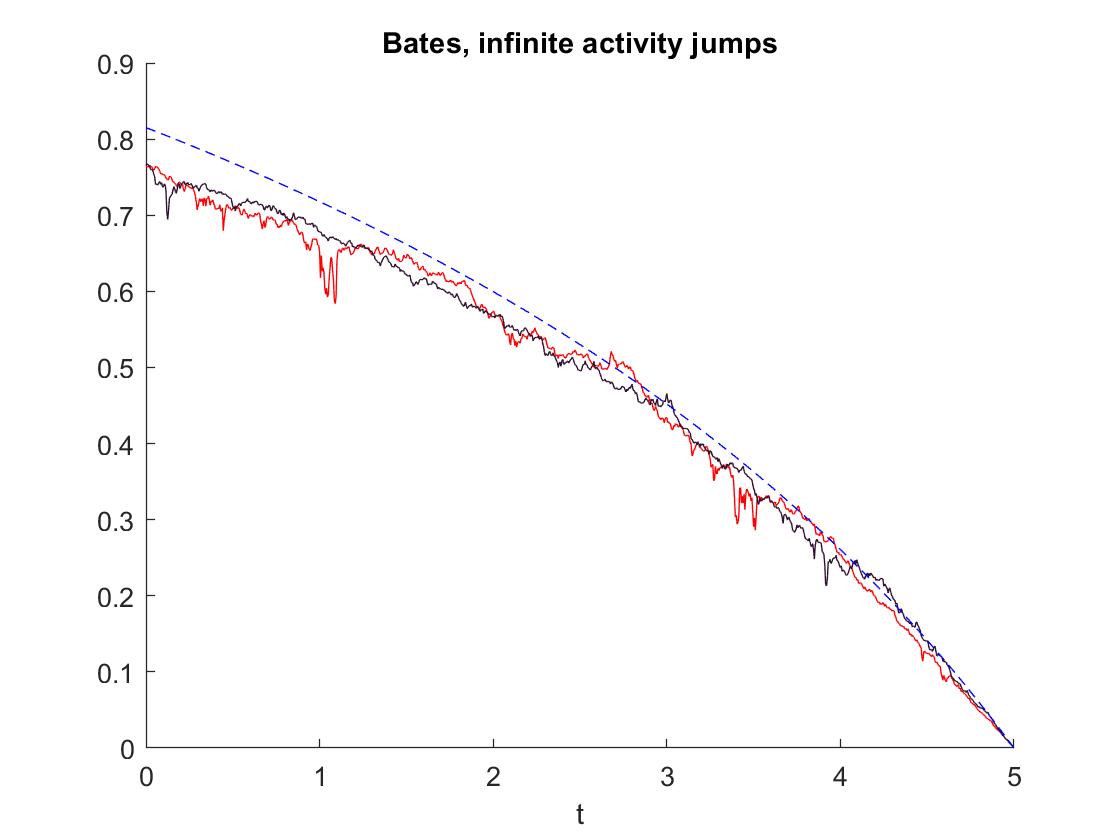
Refer to caption — Figure 1. Two samples of the strategy $\pi^{1}$ using a time discretization of $N=1000$ steps and a space discretization of $200$ steps for Matlab’s pde solver pdepe. The reference solution for the constant volatility (setting $z\equiv\theta$ ) following [41] is plotted in blue dashes.

(b)

Constant activity jumps: $\vartheta=\delta_{q}$ . This model with constant jump size $q$ (set to $l^{L}_{\max}$ ) uses the same CIR process as in the model with infinite jumps, the only difference is - according to 6.3 - the market price of risk

$\displaystyle\lambda^{2}(z)=z\alpha_{2}-\frac{q}{1-\alpha_{2}q},$

where $\alpha^{2}=\alpha^{1}=2.5$ .

Figure 2 shows the resulting strategy $\pi^{2}$ for this model.

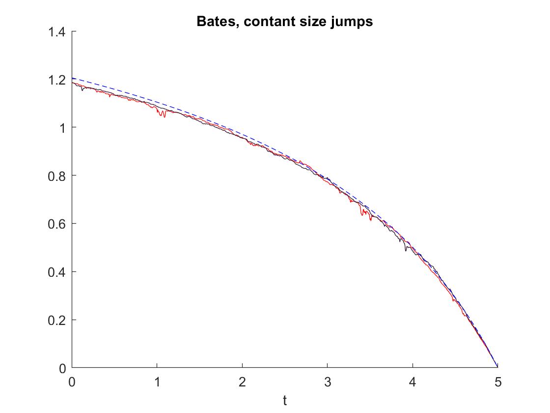
Figure 2. Two samples of the strategy $\pi^{2}$ using a time discretization of $N=1000$ steps and a space discretization of $200$ steps for Matlab’s pde solver pdepe. The reference solution for the constant volatility (setting $z\equiv\theta$ ) following [41] is plotted in blue dashes.
(c)

Absence of jumps: For the Bates model without jumps we are practically in a Heston setting. Our coefficients remain the same, except for the excess return, which just takes the form $\lambda^{3}(z)=\alpha_{3}z$ , with $\alpha_{3}=\alpha_{1}=2.5$ . We obtain the following strategies $\pi^{3}$ for this model in Figure 3.

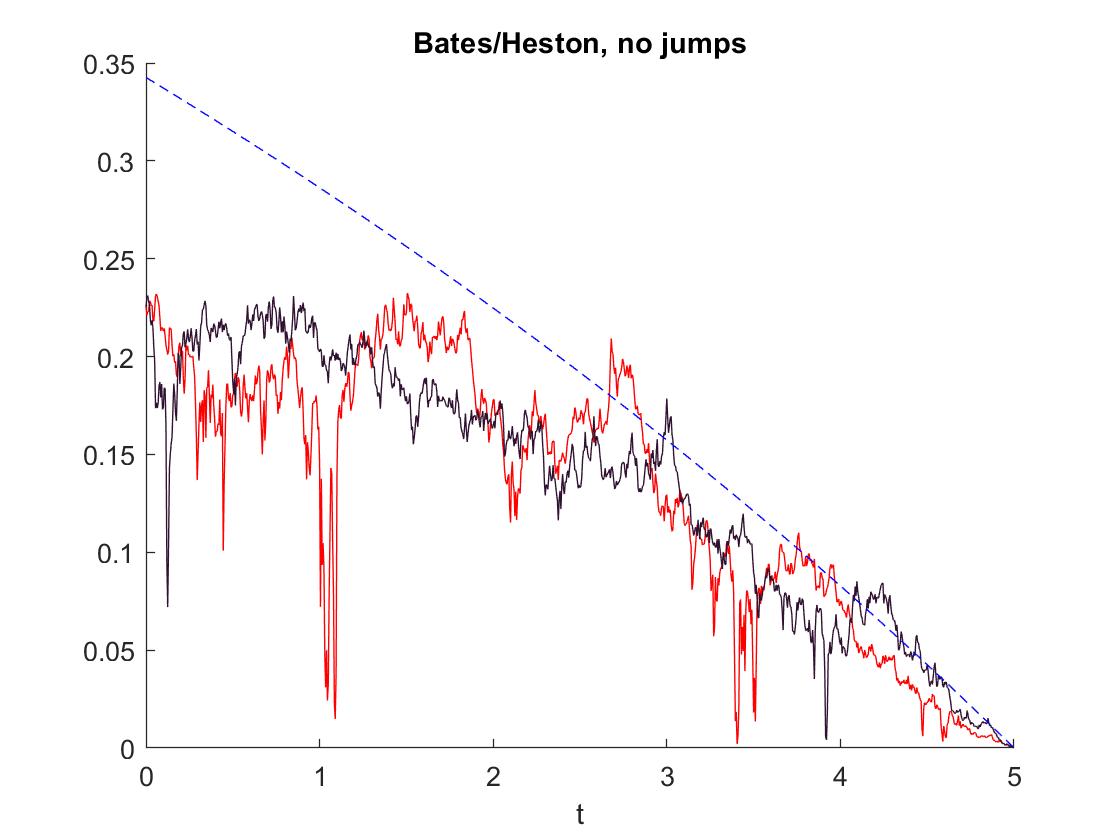
Figure 3. Two samples of the strategy $\pi^{3}$ using a time discretization of $N=1000$ steps and a space discretization of $200$ steps for Matlab’s pde solver pdepe. The reference solution for the constant volatility (setting $z\equiv\theta$ ) following [41] is plotted in blue dashes.
(d)

We continue with the ’original’ Heston model, assuming the same CIR-process as before, but keeping $\lambda^{4}$ constant at $\lambda^{4}\equiv\alpha^{4}\theta$ with $\alpha^{4}=\alpha^{1}=2.5$ . In this case, the market price of risk is not appropriate, which results in a non-constant post-crash-strategy $\pi^{M,4}=\frac{\lambda^{4}}{(\sigma^{4})^{2}\vee 0}$ which we illustrate in an additional figure. In those samples, one can see that the condition $\pi^{4}\leq\pi^{M,4}$ from Theorem 25 is violated, so we cannot guarantee that $\pi^{4}$ is an actual optimal pre-crash strategy.

Figure 4. Left: The post-crash optimal strategy $\pi^{M,4}$ for two sample paths. The peaks mount up to a value of about 1200. Right: The same sample graphs of $\pi^{M,4}$ together with the according strategy samples $\pi^{4}$ (dashed). Note that 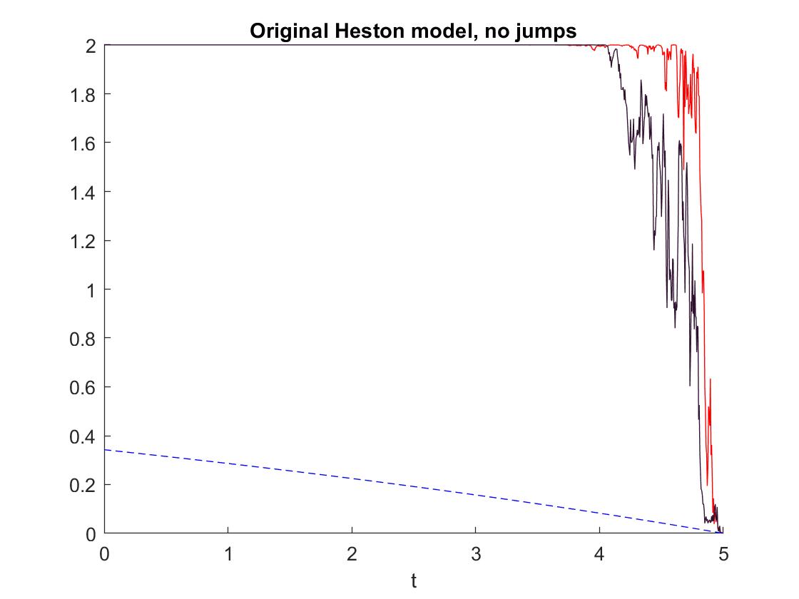$\pi^{4}\nleq\pi^{M,4}$ .

Figure 5. Two samples of the strategy $\pi^{4}$ using a time discretization of $N=1000$ steps and a space discretization of $200$ steps for Matlab’s pde solver pdepe. The reference solution for the constant volatility (setting $z\equiv\theta$ ) following [41] is plotted in blue dashes. Note that $\pi^{4}$ is quite close to the upper bound for admissibility, $2$ , here (numerically indistinguishable for the first 3 time steps even).

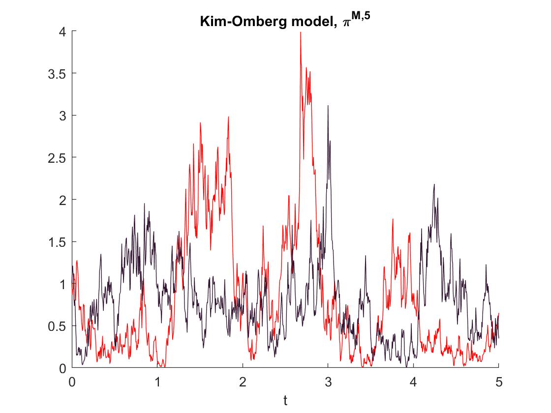
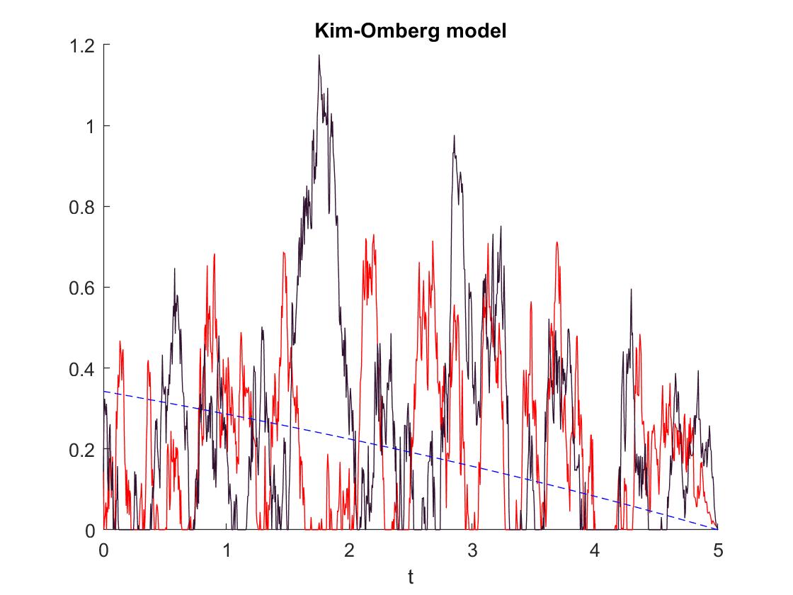
7.2. Numerics for the Kim-Omberg Model

The second model’s numerical simulations that we present here are from the Kim-Omberg model. Here, the process $\lambda^{5}\equiv z$ is given by the Ornstein-Uhlenbeck dynamics

\displaystyle dz_{t}=\kappa^{KO}(\theta^{KO}-z_{t})dt+\tilde{\varsigma}^{KO}d\hat{W}_{t},\quad z_{0}=\theta^{KO},\quad t\in[0,T],

with $\kappa^{KO}=3.5,\theta^{KO}=\theta=0.014,\tilde{\varsigma^{KO}}=0.3$ , and $\sigma^{5}\equiv\sqrt{\theta^{KO}}$ .

Also in this model, we can not guarantee the condition $\pi^{5}\leq\pi^{M,5}$ for Theorem 25.

Acknowledgements

We wish to thank the participants of the Stochastic Models and Control Workshop 2017 in Trier and from the London Mathematical Finance Seminar Series for useful comments and discussions.

References

[1] M. Altmayer and A. Neuenkirch, Discretising the Heston model: an analysis of the weak convergence rate, IMA J. Numer. Anal., 37 (2017), pp. 1930–1960.
[2] D. Applebaum, Lévy processes and stochastic calculus, Cambridge university press, 2009.
[3] G. Barles, R. Buckdahn, and É. Pardoux, Backward stochastic differential equations and integral-partial differential equations, Stochastics: An International Journal of Probability and Stochastic Processes, 60 (1997), pp. 57–83.
[4] G. Barles and P. Souganidis, Convergence of approximation schemes for fully nonlinear second order equations, Asymptotic Analysis, 4 (1991), pp. 271–283.
[5] D. Bates, Jumps and stochastic volatility: Exchange rate processes implicit in deutsche mark options, Review of Financial Studies, 9 (1996), pp. 69–107.
[6] C. Belak, S. Christensen, and O. Menkens, Worst-case optimal investment with a random number of crashes, Statistics and Probability Letters, 90 (2014), pp. 140–148.
[7] C. Belak, O. Menkens, and J. Sass, Worst-case portfolio optimization with proportional transaction costs, Stochastics, 87 (2015), pp. 623–663.
[8] N. Branger, C. Schlag, and E. Schneider, Optimal portfolios when volatility can jump, Journal of Banking & Finance, 32 (2008), pp. 1087–1097.
[9] P. Briand and F. Confortola, Bsdes with stochastic lipschitz condition and quadratic pdes in hilbert spaces, Stochastic Processes and their Applications, 118 (2008), pp. 818–838.
[10] P. Briand, B. Delyon, Y. Hu, É. Pardoux, and L. Stoica, L^p solutions of backward stochastic differential equations, Stochastic Processes and their Applications, 108 (2003), pp. 109–129.
[11] M. Broadie and Ö. Kaya, Exact simulation of stochastic volatility and other affine jump diffusion processes, Operations Research, 54 (2006), pp. 217–231.
[12] G. Chacko and L. Viceira, Dynamic consumption and portfolio choice with stochastic volatility in incomplete markets, Review of Financial Studies, 18 (2005), pp. 1369–1402.
[13] S. Cox, M. Hutzenthaler, and A. Jentzen, Local Lipschitz continuity in the initial value and strong completeness for nonlinear stochastic differential equations, arXiv:1309.5595v3, (2021).
[14] A. Cozma and C. Reisinger, Exponential integrability properties of Euler discretization schemes for the Cox-Ingersoll-Ross process, Discrete and Continuous Dynamical Systems - B, 21 (2016), pp. 3359–3377.
[15] S. Dereich, A. Neuenkirch, and L. Szpruch, An Euler-type method for the strong approximation of the Cox–Ingersoll–Ross process., Proc. R. Soc. A, 468 (2012), pp. 1105–1115.
[16] S. Desmettre, R. Korn, P. Ruckdeschel, and F. Seifried, Robust worst-case optimal investment, OR Spectrum, 37 (2015), pp. 677–701.
[17] S. Desmettre, R. Korn, and F. T. Seifried, Worst-case consumption-portfolio optimization, International Journal of Theoretical and Applied Finance, 18 (2015), p. 1550004.
[18] M. Eddahbi, I. Fakhouri, and Y. Ouknine, $L^{p}(p\geq 2)$ -solutions of generalized BSDEs with jumps and monotone generator in a general filtration, Modern Stochastics: Theory and Applications, 4 (2017), pp. 25–63.
[19] N. El Karoui and S. Huang, A general result of existence and uniqueness of backward stochastic differential equations, in Backward Stochastic Differential Equations, N. El Karoui and L. Mazliak, eds., no. 364 in Pitman research Notes in Math. Series, Longman Harlow, 1997.
[20] N. El Karoui, S. Peng, and M. C. Quenez, Backward stochastic differential equations in Finance, Mathematical Finance, 7 (1997), pp. 1–71.
[21] T. Engler and R. Korn, Worst-case portfolio optimization under stochastic interest rate risk, Risks, 2 (2014), pp. 469–488.
[22] H. Föllmer, A. Schied, and S. Weber, Robust preferences and robust portfolio choice, Mathematical Modelling and Numerical Methods in Finance (P. Ciarlet, A. Bensoussan & Q. Zhang, eds.), Handbook of Numerical Analysis, 15 (2009), pp. 22–89.
[23] T. Fujiwara and H. Kunita, Stochastic differential equations of jump type and Lévy processes in diffeomorphisms group, J. Math. Kyoto Univ., 25 (1985), pp. 71–106.
[24] C. Geiss and A. Steinicke, Existence, uniqueness and comparison results for BSDEs with Lévy jumps in an extended monotonic generator setting, Probability, Uncertainty and Quantitative Risk, 3 (2018), p. 9.
[25] M. Hefter and A. Herzwurm, Strong convergence rates for Cox-Ingersoll-Ross processes – full parameter range, Journal of Mathematical Analysis and Applications, 459 (2018), pp. 1079–1101.
[26] S. L. Heston, A closed-form solution for options with stochastic volatility with applications to bond and currency options, Review of Financial Studies, 6 (1993), pp. 327–343.
[27] P. Hua and P. Wilmott, Crash courses, Risk, 10 (1997), pp. 64–67.
[28] T. Hurd and A. Kuznetsov, Explicit formulas for Laplace transforms of stochastic integrals., Markov Process. Relat. Fields, 14 (2008), pp. 277–290.
[29] M. Hutzenthaler, A. Jentzen, and M. Noll, Strong convergence rates and temporal regularity for Cox-Ingersoll-Ross processes and Bessel processes with accessible boundaries, arXiv:1403.6385, (2014).
[30] N. Ikeda and S. Watanabe, Stochastic differential equations and diffusion processes, North Holland, 1989.
[31] J. Kallsen and J. Muhle-Karbe, Utility maximization in affine stochastic volatility models, International Journal of Theoretical and Applied Finance, 13 (2010), pp. 459–477.
[32] I. Karatzas and S. Shreve, Brownian motion and stochastic calculus., New York, Springer-Verlag, 2nd ed., 1991.
[33] T. S. Kim and E. Omberg, Dynamic nonmyopic portfolio behavior, Review of Financial Studies, 1 (1996), pp. 141–161.
[34] F. H. Knight, Risk, Uncertainty and Profit, Hart, Schaffner & Marx; Houghton Mifflin Co., 1921.
[35] R. Korn and E. Leoff, Multi-asset worst-case optimal portfolios, International Journal of Theoretical and Applied Finance, 22 (2022), p. 1950019.
[36] R. Korn and O. Menkens, Worst-case scenario portfolio optimization: a new stochastic control approach, Mathematical Methods of Operations Research, 62 (2005), pp. 123–140.
[37] R. Korn and L. Müller, Optimal dynamic reinsurance with worst-case default of the reinsurer, European Actuarial Journal, 12 (2022), pp. 879–885.
[38] , Optimal portfolios in the presence of stress scenarios a worst-case approach, Mathematics and Financial Economics, 16 (2022), pp. 153–185.
[39] R. Korn and F. T. Seifried, A worst-case approach to continuous-time portfolio optimization, Radon Series on Computational and Applied Mathematics, 8 (2009), pp. 327–345.
[40] R. Korn and M. Steffensen, On worst-case portfolio optimization, SIAM Journal on Control and Optimization, 46 (2007), pp. 2013–2030.
[41] R. Korn and P. Wilmott, Optimal portfolios under the threat of a crash, International Journal of Theoretical and Applied Finance, 05 (2002), pp. 171–187.
[42] H. Kraft, Optimal portfolios and heston’s stochastic volatility model: an explicit solution for power utility, Quantitative Finance, 5 (2005), pp. 303–313.
[43] S. Kremsner and A. Steinicke, $L^{p}$ -Solutions and Comparison Results for Lévy Driven BSDEs in a Monotonic, General Growth Setting, Journal of Theoretical Probability, (2020), p. arXiv:1909.06181.
[44] T. Kruse and A. Popier, BSDEs with monotone generator driven by Brownian and Poisson noises in a general filtration, Stochastics, 88 (2016), pp. 491–539.
[45] J. Li, Backward Stochastic Differential Equations with Unbounded Coefficients and Their Applications, PhD thesis, University of Liverpool, 2014.
[46] J. Liu, Portfolio selection in stochastic environments, The Review of Financial Studies, 20 (2007), pp. 1–39.
[47] H. Pham, Smooth solutions to optimal investment models with stochastic volatilities and portfolio constraints, Applied Mathematics and Optimization, 46 (2002), pp. 55–78.
[48] P. Protter, Stochastic Integration and Stochastic Differential Equations, Springer, Berlin, 2004.
[49] A. Saplaouras, Backward stochastic differential equations with jumps are stable, dissertation, TU Berlin, 2017.
[50] A. Schied, Optimal investments for robust utility functionals in complete market models, Mathematics of Operations Research, 30 (2005), pp. 750–764.
[51] F. T. Seifried, Optimal investment for worst-case crash scenarios: A martingale approach, Mathematics of Operations Research, 35 (2010), pp. 559–579.
[52] D. Talay and Z. Zheng, Worst case model risk management, Finance and Stochastics, 1 (2002), pp. 517–537.
[53] T. Zariphopoulou, A solution approach to valuation with unhedgeable risks, Finance and Stochastics, 5 (2001), pp. 61–82.

Appendix A Proofs from Section 3

Proof.

(Proposition 9) There are three possibilities for $\pi^{M}$ . Either $\pi^{M}=0$ or $\pi^{M}=\frac{1}{l^{L}_{\max}}$ or $\pi^{M}\in\left(0,\frac{1}{l^{L}_{\max}}\right)$ .

Define $\Psi(\lambda,\sigma,y):=\partial_{y}\Phi(y)=\lambda-\sigma^{2}y-\int_{[0,l^{L}_{\max}]}\frac{l}{1-yl}\vartheta(dl).$ In the case $\pi^{M}\in\left(0,\frac{1}{l^{L}_{\max}}\right)$ , $\Psi(\lambda,\sigma,\pi^{M})=0$ and by the implicit function theorem, as $\partial_{y}\Psi=-\sigma^{2}-\int_{[0,l^{L}_{\max}]}\frac{l^{2}}{(1-yl)^{2}}\theta(dl)<0$ , $\pi^{M}$ may be expressed by a functional relation $\pi^{M}=\psi(\lambda,\sigma)$ , where $\psi$ is differentiable in a neighborhood around $(\lambda,\sigma)$ . This shows continuity in this case. To find first Lipschitz-like relations, we start by differentiating $0=\partial_{\lambda}\Psi(\lambda,\sigma,\psi(\lambda,\sigma))$ , and obtain, using the chain rule,

\partial_{\lambda}\psi(\lambda,\sigma)=\frac{1}{\sigma^{2}+\int_{[0,l^{L}_{\max}]}\frac{l^{2}}{(1-\psi(\lambda,\sigma)l)^{2}}\theta(dl)}<\frac{1}{\sigma^{2}}<\infty.

The same works for the derivative in direction $\sigma$ ,

	$\displaystyle 0=\partial_{\sigma}\Psi(\lambda,\sigma,\psi(\lambda,\sigma))\quad\Leftrightarrow$
	$\displaystyle 0=-2\sigma\psi(\lambda,\sigma)-\left(\sigma^{2}+\int_{[0,l^{L}_{\max}]}\frac{l^{2}}{(1-\psi(\lambda,\sigma)l)^{2}}\theta(dl)\right)\partial_{\sigma}\psi(\lambda,\sigma)\quad\Leftrightarrow$
	$\displaystyle-\frac{2\sigma\psi(\lambda,\sigma)}{\sigma^{2}+\int_{[0,l^{L}_{\max}]}\frac{l^{2}}{(1-\psi(\lambda,\sigma)l)^{2}}\theta(dl)}=\partial_{\sigma}\psi(\lambda,\sigma).$

and hence, $|\partial_{\sigma}\psi(\lambda,\sigma)|\leq\frac{2}{l^{L}_{\max}|\sigma|}\leq\frac{2}{l^{L}_{\max}\inf_{\tilde{\sigma}}|\tilde{\sigma}|}$ . Trivially, also in the remaining cases, $\pi^{M}\in\{0,\tfrac{1}{l^{L}_{\max}}\}$ , it can be expressed as a function $\psi$ in $(\lambda,\sigma)$ . We show that $\psi$ is continuous, no matter what case we are in: Let $(\lambda_{n},\sigma_{n})$ be a sequence converging to some $(\lambda,\sigma)$ . Let $p^{*}$ be a limit point of a converging subsequence of $\psi(\lambda_{n_{k}},\sigma_{n_{k}})$ (which exists, as $\psi$ only takes values in $\left[0,\tfrac{1}{l^{L}_{\max}}\right]$ ). For all $k\geq 1$ is then

\Phi(\psi(\lambda_{n_{k}},\sigma_{n_{k}}))=\Phi(\lambda_{n_{k}},\sigma_{n_{k}},\psi(\lambda_{n_{k}},\sigma_{n_{k}}))\geq\Phi(\lambda_{n_{k}},\sigma_{n_{k}},\psi(\lambda,\sigma)).

Since $\Phi$ is continuous in $\lambda,\sigma,y$ , taking the limit $k\to\infty$ in the last inequality, we get

\Phi(\lambda,\sigma,p^{*})\geq\Phi(\lambda,\sigma,\psi(\lambda,\sigma)).

By the uniqueness of the $\mathrm{argmax}$ (follows from the strict convexity of $\Phi$ in $y$ ), we get $p^{*}=\psi(\lambda,\sigma).$

We show that the Lipschitz-like properties hold independently from the cases: Doing this for $\lambda$ in the sequel, the proof works the similarly for $\sigma$ . To that end, fix $\sigma$ and let $\lambda<\lambda^{\prime}$ . For an exemplary case (other cases work similar), let $\psi(\lambda,\sigma)=0$ and let $\psi(\lambda^{\prime},\sigma)\in\left(0,\tfrac{1}{l^{L}_{\max}}\right)$ . Then set $\lambda_{1}:=\inf\{t\in(\lambda,\lambda^{\prime}]:\psi(t,\sigma)>0\}$ . In the same way set $\lambda_{2}:=\inf\big{\{}t\in(\lambda_{1},\lambda^{\prime}):\psi(t,\sigma)=\tfrac{1}{l^{L}_{\max}}\big{\}}$ , and $\lambda_{3}:=\inf\big{\{}t\in[\lambda_{2},\lambda^{\prime}):\psi(t,\sigma)<\tfrac{1}{l^{L}_{\max}}\big{\}}$ and set $\lambda_{2}:=\lambda_{3}:=\lambda_{1}$ whenever the sets are empty. We observe,

	$\displaystyle\|\psi(\lambda,\sigma)-\psi(\lambda^{\prime},\sigma)\|\leq$	$\displaystyle\|\psi(\lambda,\sigma)-\psi(\lambda_{1},\sigma)\|+\|\psi(\lambda_{1},\sigma)-\psi(\lambda_{2},\sigma)\|$
		$\displaystyle+\|\psi(\lambda_{2},\sigma)-\psi(\lambda_{3},\sigma)\|+\|\psi(\lambda_{3},\sigma)-\psi(\lambda^{\prime},\sigma)\|$
		$\displaystyle=\|\psi(\lambda_{1},\sigma)-\psi(\lambda_{2},\sigma)\|+\|\psi(\lambda_{3},\sigma)-\psi(\lambda^{\prime},\sigma)\|.$

Thus, in the intervals $(\lambda_{1},\lambda_{2})$ as well as $(\lambda_{3},\lambda^{\prime})$ , $\psi$ is a differentiable function in $\lambda$ with Lipschitz constant $\frac{1}{\sigma^{2}}$ . By taking limits, this Lipschitz property extends to the intervals’ boundaries, and we obtain

\displaystyle|\psi(\lambda,\sigma)-\psi(\lambda^{\prime},\sigma)|\leq\frac{1}{\sigma^{2}}|\lambda_{1}-\lambda_{2}|+|\lambda_{3}-\lambda^{\prime}|\leq\frac{1}{\sigma^{2}}|\lambda-\lambda^{\prime}|.

If $|\sigma|\geq|\tilde{\sigma}|>0$ , Lipschitz continuity on the whole domain follows.

∎

Appendix B Proofs of BSDE results from Section 5

Proof.

(Proposition 28) In view of Subsection 5.1, the generator of the BSDE can be written as

	$\displaystyle{f}(t,y)=$
	$\displaystyle a_{t}+\frac{\lambda_{t}^{-}}{l^{WOC}}(1-e^{-(y\vee 0)})-\frac{\lambda_{t}^{+}}{l^{WOC}}(1-e^{-(y\vee 0)})+\frac{\sigma_{t}^{2}}{2\left(l^{WOC}\right)^{2}}(1-e^{-(y\vee 0)})^{2}$
	$\displaystyle-\int_{[0,l^{L}_{\max}]}\log\left(1-\frac{1-e^{-(y\vee 0)}}{l^{WOC}}l\right)\vartheta(dl),$

where $a_{t}$ is given by

\lambda_{t}\pi_{t}^{M}-\frac{\sigma_{t}^{2}(\pi_{t}^{M})^{2}}{2}+\int_{[0,l^{L}_{\max}]}\log\left(1-\pi_{t}^{M}l\right)\vartheta(dl).

Now, given the boundedness conditions on $\vartheta,\lambda,\sigma,\pi^{M}$ , the generator $f$ meets the assumptions of [24, Theorem 3.2](or e.g. [43, Theorem 3.3], [44, Theorem 1]), as seen in Subsection 5.1, (9) and (10), from which the assertion follows. ∎

Proof.

(Theorem 29) We approximate the generator ${f}$ by the functions

	$\displaystyle f^{n,N}(t,y):=$	$\displaystyle a^{N,n}_{t}+\frac{\lambda_{t}^{-}\wedge n}{l^{WOC}}(1-e^{-(y\vee 0)})-\frac{\lambda_{t}^{+}}{l^{WOC}}(1-e^{-(y\vee 0)})$
		$\displaystyle+\frac{\sigma_{t}^{2}\wedge n}{2\left(l^{WOC}\right)^{2}}(1-e^{-(y\vee 0)})^{2}-\int_{[0,l^{L}_{\max}]}\log\left(1-\frac{1-e^{-(y\vee 0)}}{l^{WOC}}l\right)\vartheta(dl),$

with $a^{N,n}_{t}:=(\lambda_{t}\wedge n)\pi_{t}^{M}-\frac{(\sigma_{t}^{2}\wedge N)(\pi_{t}^{M})^{2}}{2}+\int_{[0,l^{L}_{\max}]}\log\left(1-\pi_{t}^{M}l\right)\vartheta(dl)$ , and

	$\displaystyle f^{N}(t,y):=$	$\displaystyle a^{N}_{t}+\frac{\lambda_{t}^{-}}{l^{WOC}}(1-e^{-(y\vee 0)})-\frac{\lambda_{t}^{+}}{l^{WOC}}(1-e^{-(y\vee 0)})$
		$\displaystyle+\frac{\sigma_{t}^{2}}{2\left(l^{WOC}\right)^{2}}(1-e^{-(y\vee 0)})^{2}-\int_{[0,l^{L}_{\max}]}\log\left(1-\frac{1-e^{-(y\vee 0)}}{l^{WOC}}l\right)\vartheta(dl),$

with $a^{N}_{t}:=\lambda_{t}\pi_{t}^{M}-\frac{(\sigma_{t}^{2}\wedge N)(\pi_{t}^{M})^{2}}{2}+\int_{[0,l^{L}_{\max}]}\log\left(1-\pi_{t}^{M}l\right)\vartheta(dl)$ .

For the BSDEs with generators $f^{N,n}$ (and terminal condition $0$ ), we get solutions $(\Upsilon^{N,n},\sigma_{\Upsilon}^{N,n})$ from Proposition 28. Note that $f^{N,n}(t,\omega,y)\nearrow{f^{N}}(t,\omega,y)$ and ${f^{N}}(t,\omega,y)\searrow f(t,\omega,y)$ . We will follow this order of approximations to construct solutions. For the first approximation, by the comparison theorem (e.g. in [24, Theorem 3.4], [43, Theorem 6.1], [44, Proposition 4]), we get that $\left(\Upsilon_{t}^{N,n}(\omega)\right)_{n\geq 1}$ is a monotonically increasing family for all $t\in[0,T]$ for almost all $\omega\in\Omega$ . Thus, we can define the random variable $\Upsilon^{N}_{t}(\omega):=\lim_{n\to\infty}\Upsilon_{t}^{N,n}(\omega)$ , wherever the limit exists and $0$ on the complement.

We show that $\mathbb{E}\left[\sup_{t}|\Upsilon^{N}_{t}|^{2}\right]<\infty$ . To that end, observe first that Itô’s formula yields for all $t\in[0,T]$

	$\displaystyle\|\Upsilon_{t}^{N,n}\|^{2}+\int_{t}^{T}\|\sigma^{N,n}_{\Upsilon,s}\|^{2}ds$	$\displaystyle+\int_{0}^{T}\int_{[0,l^{L}_{\max}]}\|U^{N,n}_{\Upsilon,s}(l)\|^{2}\vartheta(dl)ds$
		$\displaystyle=\int_{t}^{T}2\Upsilon^{N,n}_{s}f^{N,n}(s,\Upsilon^{N,n}_{s})ds-\int_{t}^{T}2\Upsilon_{s}^{N,n}\sigma^{N,n}_{\Upsilon,s}d{\bar{W}}_{s}$
(21)			$\displaystyle\quad-\int_{(t,T]\times[0,l^{L}_{\max}]}\left(\left(\Upsilon^{N,n}_{s-}+U^{N,n}_{\Upsilon,s}\right)^{2}-\left(\Upsilon^{N,n}_{s-}(l)\right)^{2}\right)\tilde{\nu}(ds,dl).$

From this equation, we get by taking conditional expectations w.r.t. $\mathcal{F}_{t}$ and using Young’s inequality that for all $q\in(0,\infty)$ ,

(22)			$\displaystyle\mathbb{E}\left[\int_{0}^{T}\|\sigma^{N,n}_{\Upsilon,s}\|^{2}ds\right]+\mathbb{E}\left[\int_{0}^{T}\int_{[0,l^{L}_{\max}]}\|U^{N,n}_{\Upsilon,s}(l)\|^{2}\vartheta(dl)ds\right]$
		$\displaystyle\quad\leq\frac{1}{q}\mathbb{E}\left[\sup_{t}\|\Upsilon^{N,n}_{t}\|^{2}\right]+q\mathbb{E}\left[\int_{0}^{T}f^{N,n}(s,\Upsilon^{N,n}_{s})ds\right]^{2}.$

Further, (B) implies, together with Doob’s martingale inequality, Burkholder-Davis-Gundy’s, Young’s inequality and the fact that

\left|\left(\Upsilon^{N,n}_{s-}+U^{N,n}_{\Upsilon,s}(l)\right)^{2}-\left(\Upsilon^{N,n}_{s-}\right)^{2}\right|\leq 4\sup_{t}|\Upsilon^{N,n}_{t}||U^{N,n}_{\Upsilon,s}(l)|,

that there is a constant $c$ , such that for all $R\in(0,\infty)$ ,

	$\displaystyle\mathbb{E}\left[\sup_{t}\|\Upsilon^{N,n}_{t}\|^{2}\right]\leq\frac{1}{R}\mathbb{E}\left[\sup_{t}\|\Upsilon^{N,n}_{t}\|^{2}\right]+R\mathbb{E}\left[\int_{0}^{T}f^{N,n}(s,\Upsilon^{N,n}_{s})ds\right]^{2}$
	$\displaystyle\quad\quad\quad+4c\mathbb{E}\left[\int_{0}^{T}\left\|\Upsilon^{N,n}_{s}\sigma^{N,n}_{\Upsilon,s}\right\|^{2}ds\right]^{\frac{1}{2}}+8c\mathbb{E}\left[\int_{0}^{T}\sup_{t}\|\Upsilon^{N,n}_{t}\|^{2}\left\|U^{N,n}_{\Upsilon,s}(l)\right\|^{2}\vartheta(dl)ds\right]^{\frac{1}{2}}$
	$\displaystyle\leq\frac{1}{R}\mathbb{E}\left[\sup_{t}\|\Upsilon^{N,n}_{t}\|^{2}\right]+R\mathbb{E}\left[\int_{0}^{T}f^{N,n}(s,\Upsilon^{N,n}_{s})ds\right]^{2}$
	$\displaystyle\quad\quad+\frac{8c}{R}\mathbb{E}\left[\sup_{t}\|\Upsilon^{N,n}_{t}\|^{2}\right]+cR\mathbb{E}\left[\int_{0}^{T}\|\sigma^{N,n}_{\Upsilon,s}\|^{2}ds\right]+cR\mathbb{E}\left[\int_{0}^{T}\left\|U^{N,n}_{\Upsilon,s}(l)\right\|^{2}\vartheta(dl)ds\right],$

where we used Young’s inequality again for the second estimate. Replacing the last term with the help of inequality (22), we arrive at

	$\displaystyle\mathbb{E}\left[\sup_{t}\|\Upsilon^{N,n}_{t}\|^{2}\right]\leq$	$\displaystyle\left(\frac{1+16c}{R}+\frac{cR}{q}\right)\mathbb{E}\left[\sup_{t}\|\Upsilon^{N,n}_{t}\|^{2}\right]$
		$\displaystyle+\left(R+cRq\right)\mathbb{E}\left[\int_{0}^{T}f^{N,n}(s,\Upsilon^{N,n}_{s})ds\right]^{2}.$

Choosing now $R$ and $q$ such that $\frac{1+16c}{R}+\frac{cR}{q}<1$ , we find a constant $C\in(0,\infty)$ such that $\mathbb{E}\left[\sup_{t}|\Upsilon^{N,n}_{t}|^{2}\right]\leq C\mathbb{E}\left[\int_{0}^{T}f^{N,n}(s,\Upsilon^{N,n}_{s})ds\right]^{2}$ . From our integrability assumption on $\lambda$ and $\sigma$ follow the uniform integrability of $\left(\sup_{t}|\Upsilon^{N,n}_{t}|^{2}\right)_{n\geq 1}$ and thus also $\mathbb{E}\left[\sup_{t}|\Upsilon^{N}_{t}|^{2}\right]<\infty$ .

Now, by dominated convergence we get that for $t\in[0,T]$ ,

\lim_{n\to\infty}\int_{t}^{T}f^{N,n}(s,\Upsilon_{s}^{N,n})ds=\int_{t}^{T}f^{N}(s,\Upsilon^{N}_{s})ds,\quad\text{a.s.}

and hence

	$\displaystyle\Upsilon^{N}_{t}-\int_{t}^{T}f^{N}(s,\Upsilon^{N}_{s})ds$	$\displaystyle=\lim_{n\to\infty}\left(\Upsilon_{t}^{N,n}-\int_{t}^{T}f^{N,n}(s,\Upsilon_{s}^{N,n})ds\right)$
		$\displaystyle=\lim_{n\to\infty}\left(-\int_{t}^{T}\sigma^{N,n}_{\Upsilon,s}d{\bar{W}}_{s}-\int_{]t,T]\times[0,l^{L}_{\max}]}U^{N,n}_{\Upsilon,s}(l)\tilde{\nu}(ds,dl)\right).$

Together with the integrability assumptions on $\lambda,\sigma$ and since for all $t\in[0,T]$ , $\mathbb{E}\left[|\Upsilon^{N}_{t}|^{2}\right]<\infty$ , it follows that $\int_{t}^{T}\sigma^{N,n}_{\Upsilon,s}d{\bar{W}}_{s}+\int_{]t,T]\times[0,l^{L}_{\max}]}U^{N,n}_{\Upsilon,s}(l)\tilde{\nu}(ds,dl)$ converges in $L^{2}$ to a random variable $V_{t}\in L^{2}$ . Therefore,

0=\mathbb{E}\left[\int_{t}^{T}\sigma^{N,n}_{\Upsilon,s}d{\bar{W}}_{s}+\int_{]t,T]\times[0,l^{L}_{\max}]}U_{\Upsilon,s}(l)\tilde{\nu}(ds,dl)\middle|\mathcal{F}_{t}\right]\to\mathbb{E}\left[V_{t}\middle|\mathcal{F}_{t}\right],\quad\text{a.s.},

and $\mathbb{E}\left[V_{t}\middle|\mathcal{F}_{t}\right]=0$ follows. In particular, $V_{0}=-\Upsilon^{N}_{0}+\int_{t}^{T}f^{N}(s,\Upsilon^{N}_{s})ds\in L^{2}$ . By the martingale representation theorem, there are processes $A,B$ , $A$ progressively measurable and $B$ predictable such that

V_{0}=\int_{0}^{T}A_{s}d{\bar{W}}_{s}+\int_{(0,T]\times[0,l^{L}_{\max}]}B_{s}(l)\tilde{\nu}(ds,dl),

and

\mathbb{E}\left[\int_{0}^{T}A_{s}^{2}ds\right]+\mathbb{E}\left[\int_{0}^{T}\int_{0}^{l^{L}_{\max}}B_{s}(l)^{2}\vartheta(dl)ds\right]<\infty.

For all $t\in[0,T]$ we have $V_{0}-V_{t}=-\Upsilon^{N}_{0}+\Upsilon^{N}_{t}+\int_{0}^{t}f^{N}(s,\Upsilon^{N}_{s})ds$ , which is $\mathcal{F}_{t}$ -measurable implying $\mathbb{E}\left[V_{0}-V_{t}\middle|\mathcal{F}_{t}\right]=V_{0}-V_{t}$ . Altogether, we have that

	$\displaystyle V_{0}-V_{t}$	$\displaystyle=\mathbb{E}\left[V_{0}-V_{t}\middle\|\mathcal{F}_{t}\right]=\mathbb{E}\left[V_{0}\middle\|\mathcal{F}_{t}\right]-\mathbb{E}\left[V_{t}\middle\|\mathcal{F}_{t}\right]$
		$\displaystyle=\int_{0}^{t}A_{s}d{\bar{W}}_{s}+\int_{]0,t]\times[0,l^{L}_{\max}]}B_{s}(l)\tilde{\nu}(ds,dl)-0.$

As a consequence,

	$\displaystyle V_{0}-V_{t}$	$\displaystyle=\int_{0}^{T}A_{s}d{\bar{W}}_{s}+\int_{]0,T]\times[0,l^{L}_{\max}]}B_{s}(l)\tilde{\nu}(ds,dl)-V_{t}$
		$\displaystyle=\int_{0}^{t}A_{s}d{\bar{W}}_{s}+\int_{]0,t]\times[0,l^{L}_{\max}]}B_{s}(l)\tilde{\nu}(ds,dl),$

from which we infer $V_{t}=\int_{t}^{T}A_{s}d{\bar{W}}_{s}+\int_{]t,T]\times[0,l^{L}_{\max}]}B_{s}(l)\tilde{\nu}(ds,dl)$ . Now it is readily checked that $(\Upsilon,A,B)$ solves the BSDE given by ${f^{N}}$ , so we can set $\sigma^{N}_{\Upsilon}:=A$ and $U^{N}_{\Upsilon}:=B$ . We go over to the approximation in $N$ now. Note that for all $N\geq M$ , $n\geq 0$ and all $t\in[0,T]$ we have that $\mathbb{P}$ -a.s.

\displaystyle\Upsilon^{N,n}_{t}\geq\Upsilon^{M,n}_{t},\quad\text{hence}\quad\Upsilon^{N}_{t}\geq\Upsilon^{M}_{t}.

Therefore, we may define again for all $t$ , $\Upsilon_{t}:=\lim_{N\to\infty}\Upsilon^{N}_{t}$ on the set where the limit exists and 0 otherwise. Now the same steps from (B) can be performed again, ending up with a solution $(\Upsilon,\sigma_{\Upsilon},U_{\Upsilon})$ .

∎

Proof.

(Theorem 31) Existence follows by Theorem 29 and the variants depicted in Remark 30 as $\lambda$ and $\sigma^{2}$ allow finite moments of any order $p>0$ . Denoting differences between two supposed solutions $\Upsilon,\Upsilon^{\prime}$ by $\Delta\Upsilon:=\Upsilon-\Upsilon^{\prime}$ , we get, using the Itô formula given in [44, Lemma 7] for $p=1$ ,

\displaystyle\mathbb{E}\left[|\Delta\Upsilon_{t}|\right]\leq\mathbb{E}\left[\int_{t}^{T}|f(s,\Upsilon_{s})-f(s,\Upsilon^{\prime}_{s})|ds\right].

We now split up the set $\Omega$ into $C_{n}(t)=\left\{\omega:\frac{\lambda_{t}^{-}(\omega)}{l^{WOC}}+\frac{\sigma_{t}^{2}}{2(l^{WOC})^{2}}\leq n\right\}$ and $\Omega\setminus C_{n}(t)$ to estimate, using Lipschitz and boundedness properties of the function $y\mapsto 1-\exp(-(y\vee 0))$ ,

\displaystyle\mathbb{E}\left[|\Delta\Upsilon_{t}|\right]\leq n\int_{t}^{T}\mathbb{E}\left[\Delta|\Upsilon_{s}|\right]ds+c\mathbb{E}\left[\int_{t}^{T}\chi_{\Omega\setminus C_{n}(s)}2\left(\lambda_{s}^{-}+\sigma_{s}^{2}\right)ds\right],

where $c=\left(\frac{1}{l^{WOC}}\vee\frac{1}{2(l^{WOC})^{2}}\right)$ . Gronwall’s inequality now shows that for $r\in[t,T]$ :

\displaystyle\mathbb{E}\left[|\Delta\Upsilon_{r}|\right]\leq e^{n(T-t)}c\mathbb{E}\left[\int_{t}^{T}\chi_{\Omega\setminus C_{n}(s)}2\left(\lambda_{s}^{-}+\sigma_{s}^{2}\right)ds\right].

The terms can be further estimated, using the definition of $C_{n}$ and that $\frac{e^{ax}}{a}\geq x$ , by

\displaystyle\mathbb{E}\left[|\Delta\Upsilon_{r}|\right]\leq c\mathbb{E}\left[\int_{t}^{T}\chi_{\Omega\setminus C_{n}(s)}\frac{e^{4(T-t)\max\{1/c,1\}\left(\lambda_{s}^{-}+\sigma_{s}^{2}\right)}}{4(T-t)\max\{1/c,1\}}ds\right].

If $t_{1}$ is such that $4(T-t_{1})\max\{1/c,1\}<\varepsilon$ , then the right hand side tends to zero as $n\to\infty$ , showing that $\Delta\Upsilon=0$ on $[t_{1},T]$ . We can now perform the same steps as above for the BSDE

\Delta\Upsilon_{t}=\int_{t}^{t_{1}}\left(f(s,\Upsilon_{s})-f(s,\Upsilon^{\prime}_{s})\right)ds-\int_{t}^{t_{1}}\sigma_{\Upsilon,s}d\bar{W}_{s}-\int_{(t,t_{1}]\times[0,l^{L}_{\max}]}U_{\Upsilon,s}(l)\tilde{\nu}(ds,dl),

$t\in[0,t_{1}]$ , showing iteratively that $\Delta\Upsilon=0$ on the whole interval $[0,T]$ . Uniqueness of $\sigma_{\Upsilon}$ and $U_{\Upsilon}$ then follow. ∎

Proof.

(Theorem 32) Denoting differences $\Upsilon-\Upsilon^{\prime},\sigma_{\Upsilon}-\sigma_{\Upsilon}^{\prime},U-U^{\prime}$ by $\Delta\Upsilon,\Delta\sigma_{\Upsilon},\Delta U_{\Upsilon}$ , and letting $B(s):=\left\{l\in[0,l^{L}_{\max}]:\Delta U_{\Upsilon,s}(l)\geq-\Delta\Upsilon_{s}\right\}$ , by Tanaka-Meyer’s formula we get that

	$\displaystyle((\Delta\Upsilon_{t})^{+})^{2}=\ \xi-\xi^{\prime}+\int_{t}^{T}\chi_{\left\{\Delta\Upsilon_{s}\geq 0\right\}}\bigg{[}(\Delta\Upsilon_{s})\left(f(s,\Upsilon_{s})-f^{\prime}(s,\Upsilon^{\prime}_{s})\right)-(\Delta\sigma_{\Upsilon,s})^{2}$
	$\displaystyle-\int_{t}^{T}\int_{B(s)}(\Delta U_{\Upsilon,s}(l))^{2}\vartheta(dl)+\int_{B(s)^{c}}\left((\Delta\Upsilon_{s})^{2}+2(\Delta U_{\Upsilon,s}(l))(\Delta\Upsilon_{s})\right)\vartheta\bigg{]}ds+M(t),$

where $M(t)$ is a stochastic integral term with zero expectation. Thus, omitting negative terms, we get

\displaystyle\mathbb{E}\left[((\Delta\Upsilon_{t})^{+})^{2}\right]=\mathbb{E}\left[\int_{t}^{T}\chi_{\left\{\Delta\Upsilon_{s}\geq 0\right\}}(\Delta\Upsilon_{s})\left(f(s,\Upsilon_{s})-f^{\prime}(s,\Upsilon^{\prime}_{s})\right)ds\right].

We add and subtract $f(s,\Upsilon^{\prime}_{s})$ in the integral and get, using that $f(s,\Upsilon^{\prime}_{s})\leq f^{\prime}(s,\Upsilon^{\prime}_{s})$ ,

\displaystyle\mathbb{E}\left[((\Delta\Upsilon_{t})^{+})^{2}\right]=\mathbb{E}\left[\int_{t}^{T}\chi_{\left\{\Delta\Upsilon_{s}\geq 0\right\}}(\Delta\Upsilon_{s})\left(f(s,\Upsilon_{s})-f(s,\Upsilon^{\prime}_{s})\right)ds\right]

(this step can also be performed with inserting $f^{\prime}(s,\Upsilon_{s})$ and using the inequality $f(s,\Upsilon^{\prime}_{s})\leq f(s,\Upsilon^{\prime}_{s})$ , if this is the inequality assumed). The assumption on $f$ now implies

\displaystyle\mathbb{E}\left[((\Delta\Upsilon_{t})^{+})^{2}\right]=\mathbb{E}\left[\int_{t}^{T}K_{s}((\Delta\Upsilon_{s})^{+})^{2}\wedge K_{s}(\Delta\Upsilon_{s})^{+}ds\right]

We now split up the set $\Omega$ into $C_{n}(t)=\left\{\omega:K_{t}\leq n\right\}$ and $\Omega\setminus C_{n}(t)$ to estimate

	$\displaystyle\mathbb{E}\left[((\Delta\Upsilon_{t})^{+})^{2}\right]\leq$	$\displaystyle\ n\int_{t}^{T}\mathbb{E}\left[((\Delta\Upsilon_{s})^{+})^{2}\right]ds$
		$\displaystyle+\mathbb{E}\left[\int_{t}^{T}\chi_{\Omega\setminus C_{n}(s)}2K_{s}^{2}ds\right]+\mathbb{E}\int_{s}^{T}2((\Delta\Upsilon_{s})^{+})^{2}ds.$

Gronwall’s inequality now shows that for $r\in[t,T]$ :

\displaystyle\mathbb{E}\left[((\Delta\Upsilon_{r})^{+})^{2}\right]\leq e^{(n+2)(T-t)}\mathbb{E}\left[\int_{t}^{T}\chi_{\Omega\setminus C_{n}}2K_{s}^{2}ds\right].

The terms can be further estimated by

\displaystyle\mathbb{E}\left[((\Delta\Upsilon_{r})^{+})^{2}\right]\leq e^{(n+2)(T-t)}\mathbb{E}\left[\int_{t}^{T}\chi_{\Omega\setminus C_{n}}4e^{8(T-t)K_{s}}ds\right].

If $t_{1}$ is such that $8(T-t_{1})<\varepsilon$ , then the right hand side tends to zero as $n\to\infty$ , showing that $\Delta\Upsilon\leq 0$ on $[t_{1},T]$ . As in the proof of Theorem 31, we can now show successively that on small enough intervals the process $(\Delta\Upsilon)^{+}=0$ , from which we infer the assertion. ∎

Proof.

(Proposition 36) With $\pi^{M}$ also $\Upsilon^{M}$ is almost an Itô process, it is just extended by a term involving a local time, in particular, using Tanaka-Meyer’s formula [48, Chapter 4, Theorem 70 and Corollary 1], we have

(23)	$\displaystyle\Upsilon^{M}_{t}$	$\displaystyle=-\log(1-l^{WOC}\pi^{M}_{t})$
		$\displaystyle=-\log(1-l^{WOC}\pi^{M}_{0})+\frac{(l^{WOC})^{2}L^{\varpi}_{t}}{2}+\int_{0}^{t}\frac{l^{WOC}{\bf 1}_{[0,\infty)}}{1-l^{WOC}\pi^{M}_{s}}b_{s}(\varpi_{s})d\bar{W}_{s}$
		$\displaystyle\quad+\int_{0}^{t}\bigg{(}\frac{l^{WOC}}{1-l^{WOC}\pi^{M}_{s}}{\bf 1}_{[0,\infty)}(\varpi_{s})a_{s}+\frac{\left(l^{WOC}\right)^{2}\|b_{s}\|^{2}}{(1-l^{WOC}\pi^{M}_{s})^{2}}{\bf 1}_{[0,\infty)}(\varpi_{s})\bigg{)}ds$

where $L^{\varpi}$ is the local time at $0$ of the process $\varpi$ . By the assumptions on $\pi^{M}$ , the stochastic integrals are martingales again. We name the integrands $a_{\Upsilon},b_{\Upsilon}$ . Since the $\pi^{M}$ is post-crash optimal, $Z^{M}:=Z^{\pi^{M}}$ is just given by $Z^{M}=-\Upsilon^{M}$ and as $Z^{M}$ is by assumption a submartingale, $\Upsilon^{M}$ must be a supermartingale, that is $a_{\Upsilon,t}dt+\frac{(l^{WOC})^{2}}{2}dL^{\varpi}_{t}$ is a measure with values in $(-\infty,0]$ . We can view $(\Upsilon^{M},-b_{\Upsilon})\in\mathcal{S}^{2}\times L^{2}(\bar{W})$ then as the solution to the (slightly generalized) BSDE

\displaystyle\Upsilon^{M}_{t}=\xi-\int_{t}^{T}a_{\Upsilon,s}ds-\frac{(l^{WOC})^{2}(L^{\varpi}_{T}-L^{\varpi}_{t})}{2}+\int_{t}^{T}b_{\Upsilon,s}d\bar{W}_{s}

with driver $-a_{\Upsilon}$ , additional measure term $-\frac{(l^{WOC})^{2}}{2}dL^{\varpi}_{t}$ and terminal value $\Upsilon_{T}^{M}$ . For such generalized BSDEs with data $(f,dR)$ ( $f$ being the generator and $dR$ being an additional measure term) we may apply the comparison theorem from [18, Proposition 1] to compare it to $\hat{\pi}$ which is the solution to the indifference BSDE (8). Clearly $\Upsilon_{T}^{M}\geq 0=\hat{\Upsilon}_{T}$ . For comparison of the BSDEs it is sufficient to compare them only along the solution path of one of the two BSDEs. Here we choose comparison along $(\Upsilon^{M},-b_{\Upsilon})$ . The data of the first BSDE is, as pointed out above, $(f_{1},dR_{1})=\left(-a_{\Upsilon,t},-\frac{(l^{WOC})^{2}}{2}dL^{\varpi}_{t}\right)$ . Conversely, the driver of the second BSDE evaluated along the path of $\Upsilon^{M}_{t}$ is $\Phi_{t}(\pi_{t}^{M})-\Phi_{t}(\pi_{t}^{M})=0$ , as is its measure term. So the data of the second BSDE is $(f_{2},dR_{2})=(0,d0)$ . By recapitulating the proof of the comparison theorem [18, Proposition 1], which requires $f_{2}\leq f_{1}$ as well as $dR_{2}\leq dR_{1}$ , it is easy to see (in the proof’s last inequality) that also the condition $f_{2}ds+dR_{2}\leq f_{1}ds+dR_{1}$ is sufficient. Therefore, we can conclude $\hat{\Upsilon}\leq\Upsilon^{M}$ and as utility crash exposures are just monotone transformations of portfolio processes, this implies $\hat{\pi}\leq\pi^{M}$ . ∎

Appendix C Proofs of (CIR) results from Section 6

Proof.

(Theorem 39) For bounded $\lambda,\sigma$ we refer to [3, Theorem 3.5], since the conditions of the generator of the BSDE (8) are met.

We therefore focus on the unbounded case and follow the proof of [3, Theorem 3.4]. Let $\Upsilon^{t}_{s}(x)$ be defined by the solution of (8) on $[t,T]$ . with $\lambda_{s}=\lambda(z_{s}^{t}(x))$ , $\sigma_{t}=\sigma(z_{s}^{t}(x))$ , where $z^{t}(x)$ is the solution to the forward equation (12) starting from $z^{t}_{t}=x$ on $[t,T]$ . Define then $v(t,x):=\Upsilon^{t}_{t}(x)$ What we have to show to conduct the proof as in [3] is the continuity of $v$ , uniqueness of the family of BSDE-solutions $\left(\Upsilon^{t}(x)\right)_{(t,x)\in[0,T]\times\mathbb{R}}$ , a comparison theorem and an inequality used in their proof which we treat below. In [3], all those properties follow from the uniform Lipschitz condition for their generator functions, which does not hold in the case of our generator $f$ because $\lambda$ and $\sigma$ are unbounded.

The uniqueness of the solutions to the family of BSDEs in our case is granted by Theorem 31 and the exponential integrability condition (Bexp) on $\lambda(z_{t})$ and $\sigma(z_{t})$ . The comparison theorem needed is given by Theorem 32.

We show the continuity of $v$ : We define $\Upsilon^{t}_{s}(x):=\Upsilon^{t}_{t}(x)$ for $s\leq t$ and estimate

\displaystyle|v(t,x)-v(t^{\prime},x^{\prime})|^{2}=|\Upsilon_{0}^{t}(x)-\Upsilon_{0}^{t^{\prime}}(x^{\prime})|^{2}\leq\mathbb{E}\left[\sup_{s\in{[0,T]}}|\Upsilon^{t}_{s}(x)-\Upsilon^{t^{\prime}}_{s}(x^{\prime})|^{2}\right].

Using Itô’s formula for $|\Upsilon^{t}_{s}(x)-\Upsilon^{t^{\prime}}_{s}(x^{\prime})|^{2}$ , and subsequently Young’s inequality and Doob’s maximal inequality through standard BSDE methods, we get that

\displaystyle\mathbb{E}\left[\sup_{s\in{[0,T]}}|\Upsilon^{t}_{s}(x)-\Upsilon^{t^{\prime}}_{s}(x^{\prime})|^{2}\right]\leq\mathbb{E}\left[\int_{0}^{T}\left|\chi_{[t,T]}(s)f(s,\Upsilon^{t}_{s}(x))-\chi_{[t^{\prime},T]}(s)f(s,\Upsilon^{t^{\prime}}_{s}(x^{\prime}))\right|^{2}ds\right].

We therefore have to investigate

	$\displaystyle\int_{0}^{T}\left\|\chi_{[t,T]}(s)f(s,\Upsilon^{t}_{s}(x))-\chi_{[t^{\prime},T]}(s)f(s,\Upsilon^{t^{\prime}}_{s}(x^{\prime}))\right\|^{2}ds$
	$\displaystyle=\int_{t}^{t^{\prime}}\|f(s,\Upsilon_{s}^{t}(x))\|^{2}ds+\int_{t^{\prime}}^{T}\left\|f(s,\Upsilon^{t}_{s}(x))-f(s,\Upsilon^{t^{\prime}}_{s}(x^{\prime}))\right\|^{2}ds,$

assuming $t<t^{\prime}$ . Concerning the first summand, note first that whenever

\int_{[0,l^{L}_{\max}]}\log\left(1-\frac{l}{l^{L}_{\max}}\right)\vartheta(dl)=-\infty,

by Case 1 of the proof of Proposition 7,

	$\displaystyle\int_{[0,l^{L}_{\max}]}\log\left(1-\psi(\lambda(z_{s}(x))\sigma(z_{s}(x)))l\right)\vartheta(dl)$
	$\displaystyle\leq\psi(\lambda(z_{s}(x))\sigma(z_{s}(x)))(\lambda(z_{s}(x))-\sigma(z_{s}(x))^{2}\psi(\lambda(z_{s})\sigma(z_{s}))).$

We may then use the growth and boundedness assumptions on $\lambda,\sigma,z,\vartheta$ and the form of $\Phi$ to find a constant $C>0$ and estimate the generator by

\displaystyle|f(s,y)|^{2}\leq C\left(1+|z^{t}_{s}(x)|^{2p}\right).

As there is a $K>0$ such that

\mathbb{E}\left[\int_{0}^{T}(1+|z^{t}_{s}(x)|^{2p})ds\right]\leq\mathbb{E}\left[KT(1+|x|^{2p})ds\right]<\infty,

(granted by assumption (14)) it follows by dominated convergence that

\displaystyle\mathbb{E}\left[\int_{t}^{t^{\prime}}|f(s,\Upsilon_{s}^{t}(x))|^{2}ds\right]\to 0,\quad\text{as}\quad t\to t^{\prime}.

The generator $f$ regarded as real function in $y,\lambda,\sigma$ is continuous in all those variables (which follows from the form of $f$ , the continuity of $\Phi$ and $\psi$ , see Proposition 9). As also the $z^{t}(x)$ are continuous in $x$ and $t$ by assumption (15), the generator is continuous in $t$ and $x$ . Bounding

\displaystyle\int_{t^{\prime}}^{T}|f(s,\Upsilon_{s}^{t}(x))|^{2}ds+\int_{t^{\prime}}^{T}\left|f(s,\Upsilon^{t}_{s}(x))-f(s,\Upsilon^{t^{\prime}}_{s}(x^{\prime}))\right|^{2}ds

by $\int_{0}^{T}2KC\left(1+|x|^{2p}\right)ds$ makes dominated convergence applicable again, and we infer that $v$ is continuous in $t$ and $x$ .

As a last step, to give a sufficient relation to use the proof of [3, Theorem 3.4], we have to bound the solution to the following BSDE:

	$\displaystyle\Upsilon_{s}^{h}=$	$\displaystyle\int_{s}^{t+h}\left(\tilde{\psi}(r,z_{r}^{t}(x))+f(r,\phi(r,z_{r}^{t}(x))+\Upsilon_{r}^{h})\right)dr-\int_{s}^{t}\sigma_{\Upsilon,r}^{h}d\bar{W}_{r}$
		$\displaystyle-\int_{(s,T]\times[0,l^{L}_{\max}]}U_{\Upsilon,r}^{h}(l)\tilde{\nu}(dr,dl),\quad s\in[t,t+h],$

where $\tilde{\psi}$ and $\phi$ are $C^{2}$ -functions with polynomial growth. The same procedure as in Theorem 29 and the one in Theorem 31 shows existence and uniqueness of a solution $(\Upsilon^{h},\sigma_{\Upsilon}^{h},U_{\Upsilon}^{h})\in\mathcal{S}^{2}\times L^{2}(\bar{W})\times L^{2}(\tilde{\nu})$ as the additive terms are well behaved. Further standard estimates, derived by Itô’s formula, yield

	$\displaystyle\mathbb{E}\left[\|\Upsilon_{s}^{h}\|^{2}\right]+\frac{1}{2}\mathbb{E}\left[\int_{s}^{t+h}\|\sigma_{\Upsilon,r}^{h}\|^{2}dr+\int_{s}^{t+h}\int_{[0,l^{L}_{\max}]}\|U_{\Upsilon,r}^{h}(l)\|\vartheta(dl){dr}\right]$
	$\displaystyle\leq\mathbb{E}\left[\int_{s}^{t+h}\|\Upsilon_{r}^{h}\|\left\|\tilde{\psi}(r,z_{r}^{t}(x))+f\left(r,\phi(r,z_{r}^{t}(x))+\Upsilon_{r}^{h}\right)\right\|dr\right].$

The polynomial growth of $\tilde{\psi}$ , the bounds for the moments of $z_{r}^{t}(x)$ and the since $|f(s,y)|$ is bounded by $C(1+|\lambda(z^{t}_{s}(x))|+\sigma(z^{t}_{s}(x))^{2})$ implies that there is a constant $c$ such that

	$\displaystyle\mathbb{E}\left[\|\Upsilon_{s}^{h}\|^{2}\right]+\frac{1}{2}\mathbb{E}\left[\int_{s}^{t+h}\|\sigma_{\Upsilon,r}^{h}\|^{2}dr+\int_{s}^{t+h}\int_{[0,l^{L}_{\max}]}\|U_{\Upsilon,r}^{h}(l)\|\vartheta(dl){dr}\right]$
	$\displaystyle\leq c\mathbb{E}\left[\int_{s}^{t+h}\|\Upsilon_{r}^{h}\|\left(1+\|\Upsilon_{r}^{h}\|+\|\lambda(z^{t}_{s}(x))\|+\sigma(z^{t}_{s}(x))^{2}\right)dr\right].$

Since $\lambda,\sigma$ grow at most polynomially and $z^{t}(x)$ obeys (14), it follows that

\mathbb{E}\left[|\Upsilon_{s}^{h}|^{2}\right]\leq C\mathbb{E}\left[\int_{s}^{t+h}\left(|\Upsilon_{r}^{h}|+|\Upsilon_{r}^{h}|^{2}\right)dr\right],

and, recalling that $\mathbb{E}\left[\sup_{s\in[0,T]}|Y^{h}_{s}|\right]<\infty$ , we end up with

\mathbb{E}\left[|\Upsilon_{s}^{h}|^{2}\right]\leq\tilde{C}h.

From this point on, the proof can now be performed just as the one of [3, Theorem 3.4]. ∎

Proof.

(Proposition 40) Inequality (18) follows by similar but easier calculations as in Lemma 2.1 of [23] since the square root function fulfills the inequality $\sqrt{x}\leq 1+x$ . To show inequality (19), we first define

	$\displaystyle z_{r}^{t}(x)-z_{r}^{t}(x^{\prime})-(x-x^{\prime})$	$\displaystyle=\int_{t}^{r}\!\kappa\left(z_{u}^{t}(x)-z_{u}^{t}(x^{\prime})\right)du+\tilde{\varsigma}\!\int_{t}^{r}\left(\sqrt{z_{u}^{t}(x)}-\sqrt{z_{u}^{t}(x^{\prime})}\right)d\hat{W}_{u}$
		$\displaystyle=:A_{r}+M_{r}.$

Then,

\displaystyle\mathbb{E}\left[\sup_{r\in[t,s]}\left|z_{r}^{t}(x)-z_{r}^{t}(x^{\prime})-(x-x^{\prime})\right|^{p}\right]\leq C_{p}\left(\mathbb{E}\left[\sup_{r\in[t,s]}\left|A_{r}\right|^{p}\right]+\mathbb{E}\left[\sup_{r\in[t,s]}\left|M_{r}\right|^{p}\right]\right).

Since $A$ has Lipschitz coefficients, we obtain

\displaystyle\mathbb{E}\left[\sup_{r\in[t,s]}\left|A_{r}\right|^{p}\right]\leq\kappa\left|t-s\right|^{p-1}\int_{t}^{s}\mathbb{E}\left[\left|z_{u}^{t}(x)-z_{u}^{t}(x^{\prime})\right|^{p}\right]du

by Jensen’s inequality. With Doob’s maximal inequality and Itô’s formula applied to $x\mapsto|x|^{p}$ , we get constants $C_{p,1},C_{p,2}>0$ (we will continue to number appearing $p$ -dependent constants by $C_{p,i}$ )

(24)		$\displaystyle\mathbb{E}\left[\sup_{r\in[t,s]}\left\|M_{r}\right\|^{p}\right]$	$\displaystyle\leq C_{p}\mathbb{E}\left[\left\|M_{s}\right\|^{p}\right]$
(24)			$\displaystyle\leq\tilde{C}_{p}\mathbb{E}\left[\int_{t}^{s}\|M_{u}\|^{p-2}\tilde{\varsigma}^{2}\left\|\sqrt{z_{u}^{t}(x)}-\sqrt{z_{u}^{t}(x^{\prime})}\right\|^{2}du\right]$

Next, we look at the Lamperti transformation. Therefore, we apply Lemma 3.2 from [29] to $\sqrt{z_{u}^{t}(x)}$ (or $\sqrt{z_{u}^{t}(x^{\prime})}$ respectively). We get

(25)	$\displaystyle\sqrt{z_{u}^{t}(x)}$	$\displaystyle=\sqrt{x}+\int_{t}^{u}\left(\frac{4\kappa\theta-\tilde{\varsigma}^{2}}{8}\frac{1}{\sqrt{z_{r}^{t}(x)}}-\frac{\kappa}{2}\sqrt{z_{r}^{t}(x)}\right){1}_{\left\{\sqrt{z_{r}^{t}(x)}\in(0,\infty)\right\}}dr$
		$\displaystyle\qquad+\frac{\tilde{\varsigma}}{2}\left(\hat{W}_{u}-\hat{W}_{t}\right)$
		$\displaystyle=\sqrt{x}+\int_{t}^{u}g\left(\sqrt{z_{r}^{t}(x)}\right)dr+\frac{\tilde{\varsigma}}{2}\left(\hat{W}_{u}-\hat{W}_{t}\right)$

where we set

\displaystyle g(x):=\left(\frac{\alpha}{x}+\beta x\right){1}_{\{x>0\}}

with

\displaystyle\alpha=\frac{4\kappa\theta-\tilde{\varsigma}^{2}}{8},\qquad\beta=-\frac{\kappa}{2}.

Note that $g$ satisfies the following inequality for $\alpha>0,x,x^{\prime}\geq 0$ and $\beta\in\mathbb{R}$ :

(26)

(x-x^{\prime})(g(x)-g(x^{\prime}))\leq\beta(x-x^{\prime})^{2}+\alpha\left({1}_{\{x=0\}}+{1}_{\{x^{\prime}=0\}}\right)

without the second term on the right side, this would be the so-called one-sided Lipschitz continuity (see e.g. [15]). From (25), we have

\displaystyle\sqrt{z_{u}^{t}(x)}-\sqrt{z_{u}^{t}(x^{\prime})}=\sqrt{x}-\sqrt{x^{\prime}}+\int_{t}^{u}g\left(\sqrt{z_{r}^{t}(x)}\right)-g\left(\sqrt{z_{r}^{t}(x^{\prime})}\right)dr

and by Ito’s formula, we get

	$\displaystyle\left(\sqrt{z_{u}^{t}(x)}-\sqrt{z_{u}^{t}(x^{\prime})}\right)^{2}$	$\displaystyle=\left(\sqrt{x}-\sqrt{x^{\prime}}\right)^{2}$
		$\displaystyle+2\int_{s}^{u}\left(\sqrt{z_{r}^{t}(x)}-\sqrt{z_{r}^{t}(x^{\prime})}\right)\left(g\left(\sqrt{z_{r}^{t}(x)}\right)-g\left(\sqrt{z_{r}^{t}(x^{\prime})}\right)\right)dr.$

Since $g$ fulfills inequality (26), we obtain

\displaystyle\left(\sqrt{z_{u}^{t}(x)}-\sqrt{z_{u}^{t}(x^{\prime})}\right)^{2}\leq\left(\sqrt{x}-\sqrt{x^{\prime}}\right)^{2}+2\alpha\int_{t}^{u}\left({1}_{\left\{\sqrt{z_{r}^{t}(x)}=0\right\}}+{1}_{\left\{\sqrt{z_{r}^{t}(x^{\prime})}=0\right\}}\right)dr

since $\beta<0$ . Furthermore, note that the second term on the right is $0$ $\mathbb{P}$ -a.s. by Lemma 3.1 in [29]. Inserting this into (24) and applying Young’s inequality, we get

	$\displaystyle\mathbb{E}\left[\sup_{r\in[t,s]}\left\|M_{r}\right\|^{p}\right]$	$\displaystyle\leq C_{p,3}\mathbb{E}\left[\int_{t}^{s}\|M_{u}\|^{p-2}\left(\sqrt{x}-\sqrt{x^{\prime}}\right)^{2}du\right]$
		$\displaystyle\leq C_{p,4}\mathbb{E}\left[\int_{t}^{s}\|M_{u}\|^{p}+\left\|\sqrt{x}-\sqrt{x^{\prime}}\right\|^{p}du\right]$
		$\displaystyle\leq C_{p,5}\left((s-t)\left\|\sqrt{x}-\sqrt{x^{\prime}}\right\|^{p}+\int_{t}^{s}\mathbb{E}\left[\sup_{r\in[t,u]}\left\|M_{r}\right\|^{p}\right]du\right).$

Applying Gronwall’s inequality gives

\displaystyle\mathbb{E}\left[\sup_{r\in[t,s]}\left|M_{r}\right|^{p}\right]\leq C_{p,6}(s-t)\left|\sqrt{x}-\sqrt{x^{\prime}}\right|^{p}

Summarizing, we have

	$\displaystyle\mathbb{E}\left[\sup_{r\in[t,s]}\left\|z_{r}^{t}(x)-z_{r}^{t}(x^{\prime})-(x-x^{\prime})\right\|^{p}\right]$
	$\displaystyle\leq C_{p,7}\left(\int_{t}^{s}\mathbb{E}\left[\left\|z_{u}^{t}(x)-z_{u}^{t}(x^{\prime})\right\|^{p}\right]du+(s-t)\left\|\sqrt{x}-\sqrt{x^{\prime}}\right\|^{p}\right)$
	$\displaystyle\leq C_{p,8}\left((s-t)\left\|x-x^{\prime}\right\|^{p}+(s-t)\left\|\sqrt{x}-\sqrt{x^{\prime}}\right\|^{p}\right.$
	$\displaystyle\left.\qquad\qquad+\int_{t}^{s}\mathbb{E}\left[\sup_{r\in[t,u]}\left\|z_{r}^{t}(x)-z_{r}^{t}(x^{\prime})-(x-x^{\prime})\right\|^{p}\right]du\right).$

Applying Gronwall’s inequality finishes the proof of (19). To prove (20), we can assume $x\geq x^{\prime}$ without loss of generality. Then,

\displaystyle\mathbb{P}\left(z_{t}(x)\geq z_{t}(x^{\prime}),\text{for all }0\leq t<\infty\right)=1

by Proposition 5.2.18 in [32]. Then, we have

\displaystyle\mathbb{E}\left[\left|z_{t}(x)-z_{t}(x^{\prime})\right|\right]=\mathbb{E}\left[z_{t}(x)-z_{t}(x^{\prime})\right]=(x-x^{\prime})e^{-\kappa t}

since $z_{t}(x)$ is non-central chi-square distributed with expectation $\theta+(x-\theta)e^{-\kappa t}$ . ∎

Proof.

(Proposition 43)
By (17), we get that for a starting value $x$ of $z$ ,

\displaystyle\exp(\varepsilon z_{t})=\exp\bigg{(}\varepsilon x+\varepsilon\kappa\theta t-\varepsilon\kappa\int_{0}^{t}z_{s}ds+\varepsilon\tilde{\varsigma}\int_{0}^{t}\sqrt{z_{s}}d\hat{W}_{s}\bigg{)}.

Proposition 3.2 in [14] states that

\displaystyle\sup_{t\in[0,T]}\mathbb{E}\bigg{[}-\varepsilon\kappa\int_{0}^{t}z_{s}ds+\varepsilon\tilde{\varsigma}\int_{0}^{t}\sqrt{z_{s}}d\hat{W}_{s}\bigg{]}<\infty,\quad\text{if}\quad-\kappa\varepsilon+\frac{\varepsilon^{2}\tilde{\varsigma}^{2}}{2}<0,

which is the case if $\varepsilon$ is chosen smaller than $\frac{2\kappa}{\tilde{\varsigma}^{2}}$ . ∎

	$\displaystyle\|\psi(\lambda,\sigma)-\psi(\lambda^{\prime},\sigma)\|\leq$	$\displaystyle\|\psi(\lambda,\sigma)-\psi(\lambda_{1},\sigma)\|+\|\psi(\lambda_{1},\sigma)-\psi(\lambda_{2},\sigma)\|$
		$\displaystyle+\|\psi(\lambda_{2},\sigma)-\psi(\lambda_{3},\sigma)\|+\|\psi(\lambda_{3},\sigma)-\psi(\lambda^{\prime},\sigma)\|$
		$\displaystyle=\|\psi(\lambda_{1},\sigma)-\psi(\lambda_{2},\sigma)\|+\|\psi(\lambda_{3},\sigma)-\psi(\lambda^{\prime},\sigma)\|.$

	$\displaystyle\mathbb{E}\left[\sup_{t}\|\Upsilon^{N,n}_{t}\|^{2}\right]\leq\frac{1}{R}\mathbb{E}\left[\sup_{t}\|\Upsilon^{N,n}_{t}\|^{2}\right]+R\mathbb{E}\left[\int_{0}^{T}f^{N,n}(s,\Upsilon^{N,n}_{s})ds\right]^{2}$
	$\displaystyle\quad\quad\quad+4c\mathbb{E}\left[\int_{0}^{T}\left\|\Upsilon^{N,n}_{s}\sigma^{N,n}_{\Upsilon,s}\right\|^{2}ds\right]^{\frac{1}{2}}+8c\mathbb{E}\left[\int_{0}^{T}\sup_{t}\|\Upsilon^{N,n}_{t}\|^{2}\left\|U^{N,n}_{\Upsilon,s}(l)\right\|^{2}\vartheta(dl)ds\right]^{\frac{1}{2}}$
	$\displaystyle\leq\frac{1}{R}\mathbb{E}\left[\sup_{t}\|\Upsilon^{N,n}_{t}\|^{2}\right]+R\mathbb{E}\left[\int_{0}^{T}f^{N,n}(s,\Upsilon^{N,n}_{s})ds\right]^{2}$
	$\displaystyle\quad\quad+\frac{8c}{R}\mathbb{E}\left[\sup_{t}\|\Upsilon^{N,n}_{t}\|^{2}\right]+cR\mathbb{E}\left[\int_{0}^{T}\|\sigma^{N,n}_{\Upsilon,s}\|^{2}ds\right]+cR\mathbb{E}\left[\int_{0}^{T}\left\|U^{N,n}_{\Upsilon,s}(l)\right\|^{2}\vartheta(dl)ds\right],$

(24)		$\displaystyle\mathbb{E}\left[\sup_{r\in[t,s]}\left\|M_{r}\right\|^{p}\right]$	$\displaystyle\leq C_{p}\mathbb{E}\left[\left\|M_{s}\right\|^{p}\right]$
(24)			$\displaystyle\leq\tilde{C}_{p}\mathbb{E}\left[\int_{t}^{s}\|M_{u}\|^{p-2}\tilde{\varsigma}^{2}\left\|\sqrt{z_{u}^{t}(x)}-\sqrt{z_{u}^{t}(x^{\prime})}\right\|^{2}du\right]$

	$\displaystyle\mathbb{E}\left[\sup_{r\in[t,s]}\left\|M_{r}\right\|^{p}\right]$	$\displaystyle\leq C_{p,3}\mathbb{E}\left[\int_{t}^{s}\|M_{u}\|^{p-2}\left(\sqrt{x}-\sqrt{x^{\prime}}\right)^{2}du\right]$
		$\displaystyle\leq C_{p,4}\mathbb{E}\left[\int_{t}^{s}\|M_{u}\|^{p}+\left\|\sqrt{x}-\sqrt{x^{\prime}}\right\|^{p}du\right]$
		$\displaystyle\leq C_{p,5}\left((s-t)\left\|\sqrt{x}-\sqrt{x^{\prime}}\right\|^{p}+\int_{t}^{s}\mathbb{E}\left[\sup_{r\in[t,u]}\left\|M_{r}\right\|^{p}\right]du\right).$

	$\displaystyle\mathbb{E}\left[\sup_{r\in[t,s]}\left\|z_{r}^{t}(x)-z_{r}^{t}(x^{\prime})-(x-x^{\prime})\right\|^{p}\right]$
	$\displaystyle\leq C_{p,7}\left(\int_{t}^{s}\mathbb{E}\left[\left\|z_{u}^{t}(x)-z_{u}^{t}(x^{\prime})\right\|^{p}\right]du+(s-t)\left\|\sqrt{x}-\sqrt{x^{\prime}}\right\|^{p}\right)$
	$\displaystyle\leq C_{p,8}\left((s-t)\left\|x-x^{\prime}\right\|^{p}+(s-t)\left\|\sqrt{x}-\sqrt{x^{\prime}}\right\|^{p}\right.$
	$\displaystyle\left.\qquad\qquad+\int_{t}^{s}\mathbb{E}\left[\sup_{r\in[t,u]}\left\|z_{r}^{t}(x)-z_{r}^{t}(x^{\prime})-(x-x^{\prime})\right\|^{p}\right]du\right).$

Worst-Case Optimal Investment in Incomplete Markets

Abstract.

1. Introduction

2. Financial Market Model and Worst-Case Optimization Problem

Definition 1.

Remark 2.

Remark 3.

Admissible portfolio processes

Definition 4.

Remark 5.

Lemma 6.

Proof.

3. Solution to the Post-Crash Problem

Proposition 7 (Solution of the post-crash problem).

Proof.

Corollary 8.

Proposition 9.

Definition 10.

Remark 11 (Power utility with stochastic coefficients).

4. Solution to the Pre-Crash Problem

Problem 12 (Pre-Crash Problem).

Remark 13.

Definition 14 (Worst-case dominance).

Lemma 15.

Proof.

4.1. Super- and Subindifference Strategies

Definition 16 (Super-/Subindifference Strategy).

Remark 17.

Definition 18.

Remark 19.

Lemma 20.

Proof.

4.2. The Subindifference Frontier

Proposition 21 (Subindifference Frontier).

Proof.

Remark 22.

4.3. A Superindifference Frontier Result

Proposition 23 (Superindifference Frontier).

Proof.

4.4. The Merton Bound

Lemma 24 (Merton bound).

Proof.

4.5. Worst-Case Optimality of Indifference Strategies

Theorem 25.

Proof.

5. A BSDE Characterisation of Indifference Strategies

5.1. Analysis of the Generator

Proposition 26.

Proof of Proposition 26.

Remark 27.

5.2. Solutions to the Indifference Utility BSDE

Proposition 28.

Theorem 29.

Remark 30.

Theorem 31.

Theorem 32.

Remark 33.

5.3. Existence of Indifference Strategies

Corollary 34 (Uniqueness of indifference strategies).

Lemma 35.

Proof.

Proposition 36.

Corollary 37.

6. The Markovian Case

6.1. From BSDEs to associated PDEs

Proposition 38.

Theorem 39.

6.2. Concrete Examples

Proposition 40.

Remark 41.

Proposition 42.

Proposition 43.

6.3. Modeling the Jumps

7. Numerical Experiments

7.1. Numerics for the Bates and Heston model

7.2. Numerics for the Kim-Omberg Model

Acknowledgements

References

Appendix A Proofs from Section 3

Proof.

Worst-Case Optimal Investment
in Incomplete Markets