Woven Graph Codes:
Asymptotic Performances and Examples
Abstract
Constructions of woven graph codes based on constituent block and convolutional codes are studied. It is shown that within the random ensemble of such codes based on -partite, -uniform hypergraphs, where depends only on the code rate, there exist codes satisfying the Varshamov-Gilbert (VG) and the Costello lower bound on the minimum distance and the free distance, respectively. A connection between regular bipartite graphs and tailbiting codes is shown. Some examples of woven graph codes are presented. Among them an example of a rate woven graph code with based on Heawood’s bipartite graph and containing constituent rate convolutional codes with overall constraint lengths is given. An encoding procedure for woven graph codes with complexity proportional to the number of constituent codes and their overall constraint length is presented.
Index terms—Convolutional codes, girth, graphs, graph codes, hypergraphs, LDPC codes, tailbiting codes, woven codes.
I Introduction
Woven graph codes can be considered as a generalization of low-density parity-check (LDPC) block codes [1]. Their structure as graph codes makes them suitable for iterative decoding. Moreover, the LDPC block codes are known as codes with low-complexity decoding and they can be considered as competitors to the turbo codes [2] which are sometimes called parallel concatenated codes. As mentioned in [3], the underlying graph defines a permutation of the information symbols which resembles the interleaving in turbo coding schemes.
On the other hand, similarly to the LDPC codes, graph codes usually have minimum distances essentially smaller than those of the best known linear codes of the same parameters. At a first glance, the minimum distance of a graph code does not play an important role in iterative decoding since the error-correcting capability of this suboptimal procedure is often less than that guaranteed by the minimum distance. However, in general, the belief-propagation decoding algorithms work better if the girth of the underlying graph is large, that is, if the minimum distance of the graph code is large [4].
In the sequel we distinguish between graph, graph-based, and woven graph codes. We say that a graph code is a block code whose parity-check matrix coincides with the incidence matrix of the corresponding graph. Graph-based codes constitute a class of concatenated codes with constituent block codes concatenated with a graph code (see, for example, [3]). Each vertex in the underlying graph corresponds to a constituent block code. The main feature of these codes is that the block length of their constituent block codes coincides with the degree of the underlying graph.
We introduce woven graph codes which are, in fact, graph-based codes with constituent block codes whose block length is a multiple of the graph degree , that is, their block length is , where is an integer. In particular, when tends to infinity we obtain convolutional constituent codes.
Distance properties of bipartite graph-based codes with constituent block codes were studied in [3]. It was shown that if the minimum distance of the constituent block codes is larger than or equal to , then there exist asymptotically good codes with fixed constituent codes among these graph-based codes. Also it was shown in [3] that for some range of rates, random graph-based codes with block constituent codes satisfy the VG bound when the block length of the constituent codes tends to infinity. One disadvantage of graph-based codes that becomes apparent in the asymptotic analysis is that good performances can only be achieved when the block length of the constituent block codes (which in this case coincides with the graph degree ) tends to infinity. In practice this leads to rather long graph-based codes with not only rather high decoding complexity of the iterative decoding procedures but also high encoding complexity.
In this paper, we consider a class of the generalized graph-based codes which we call woven graph codes with constituent block and convolutional codes. They are based on -partite, -uniform hypergraphs. Notice that graph-based codes with constituent block codes based on hypergraphs were considered in [5], [6]. It is mentioned in [5] that Gallager’s LDPC codes are graph codes over hypergraphs.
We consider first woven graph codes with constituent block codes. A product-type lower bound on the minimum distance of such codes is derived. In order to analyze their asymptotic performances we modify the approach used in [3] to -partite, -uniform hypergraphs and constituent block codes111When we were preparing this paper we were informed that the possibility of achieving the VG bound by considering hypergraphs was known to A. Barg [7].. It is shown that when grows to infinity in the random ensemble of woven graph codes with binary constituent block codes we can find such that there exist codes satisfying the VG lower bound on the minimum distance for any rate.
In order to generalize the asymptotic analysis to woven graph codes with constituent convolutional codes we assume that the binary constituent block code is chosen as a zero-tail (ZT) terminated convolutional code and consider a sequence of ZT convolutional codes of increasing block length . It is shown that when the overall constraint length of the woven graph code tends to infinity in the random ensemble of such convolutional codes we can find such that there exist codes satisfying the Costello lower bound on the free distance for any rate.
We also describe the constituent convolutional codes as block codes over the field of binary Laurent series [8]. This description as well as the notion of block Hamming distance [9] of convolutional codes is used to derive a product-type lower bound on the free distance of woven graph codes with constituent convolutional codes and to construct examples of such woven codes with rate . For a given hypergraph the free distance of the woven graph code depends on the numbering of code symbols associating to the hypergraph vertices. By a search over all possible permutations of the constituent code we found an example of a rate woven graph code with overall constraint length and free distance . The rate woven graph code is based on Heawood’s bipartite graph [10], [11] and contains constituent convolutional codes with overall constraint length and free distance .
We consider also the encoding problem for graph and woven graph codes. The traditional encoding technique for graph codes has complexity , where is the blocklength. We show by examples that some regular block graph codes are quasi-cyclic and thereby can be interpreted as tailbiting (TB) codes (see, for example, [12], [13]). It is known that the encoding complexity of such codes is proportional to the overall constraint length of the parent convolutional code.
By using a TB representation for the graph code we can construct an example of an encoder for a woven graph code that is also represented in the form of a TB code but with overall constraint length less than or equal to , where is the number of constituent convolutional codes with overall constraint length each.
In Section II, we consider some properties of -partite, -uniform, -regular hypergraphs. We define woven graph codes with constituent block codes as well as with constituent convolutional codes and obtain product-type lower bounds on their minimum and free distances. Then, in Section III, we derive a lower bound on the free distance of the random ensemble of woven graph codes. In Section IV, examples of woven graph codes are given. We conclude the paper by considering encoding techniques for graph codes and woven graph codes in Section V.
II Preliminaries
A hypergraph is a generalization of a graph in which the edges are subsets of vertices and may connect (contain) any number of vertices. These edges are called hyperedges. A hypergraph is called -uniform if every hyperedge has cardinality or, in other words, connects vertices. If the hypergraph is simply a graph. The degree of a vertex in a hypergraph is the number of hyperedges that are connected to (contain) it. If all vertices have the same degree we say that this is the degree of the hypergraph. The hypergraph is -regular if every vertex has the same degree .
Let the set of vertices of an -uniform hypergraph be partitioned into disjoint subsets , . A hypergraph is said to be -partite if no edge contains two vertices from the same set , .
In the sequel we consider -partite, -uniform, -regular hypergraphs. Such a hypergraph is a union of disjoint subsets of vertices. Each vertex has no connections in its own set and is connected with vertices in the other subsets.
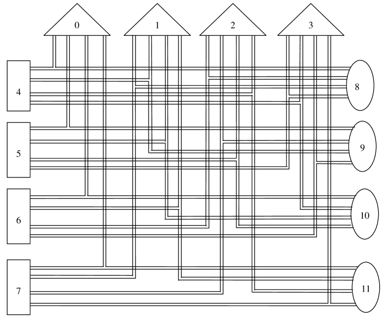
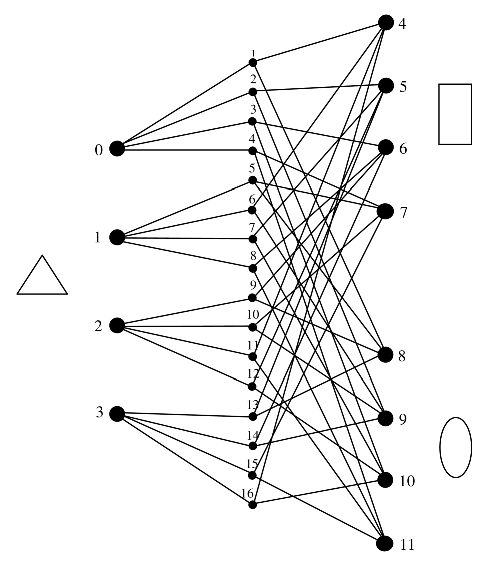
In Fig. 1 a -partite, -uniform, -regular hypergraph is shown. It contains three sets of vertices. They are shown by triangles, rectangles, and ovals, respectively. There are no edges connecting vertices inside any of these three sets. The vertices are connected by hyperedges each of which connects three vertices.
A cycle of length in the hypergraph is an alternating sequence of vertices and hyperedges where all vertices are distinct except the initial and the final vertex, which coincide, and all edges are distinct. The girth of a hypergraph is the length of its shortest cycle.
In Fig. 2 we show a subgraph that contains the shortest cycle of the -partite, -uniform, -regular hypergraph in Fig. 1. It consists of the vertices , , and and has girth equal to 2. We introduce the notion of a compact -connected subgraph in the hypergraph. It is a connected subgraph in which each vertex is incident with at least hyperedges. We call the length (number of hyperedges) of the shortest compact subgraph its (,)-girth. In Fig. 2 the hyperedges belonging to the shortest -compact subgraph are marked by circles. It is easy to see that (,)-girth is .
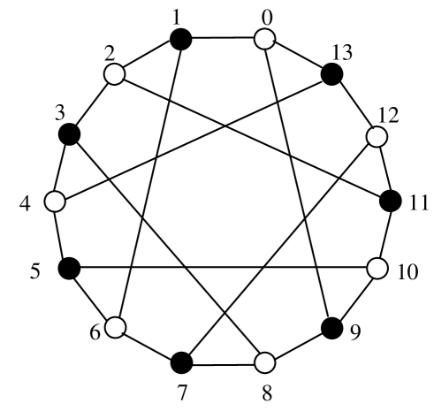
A -partite, -uniform hypergraph is a bipartite graph. For such a hypergraph the (,)-girth is equal to the girth and a compact subgraph is a cycle. Heawood’s bipartite graph [10], [11] with vertices and edges is shown in Fig. 3. This graph contains a set of black and a set of white vertices. Each vertex has no connections within its own set and is connected with vertices from the other set. The girth of the Heawood graph is .
II-A Graph-based codes and graph codes
In order to illustrate the structure of a binary graph-based block code with constituent block codes we represent the Heawood bipartite graph using a so-called Tanner graph [15] as shown in Fig. 4.
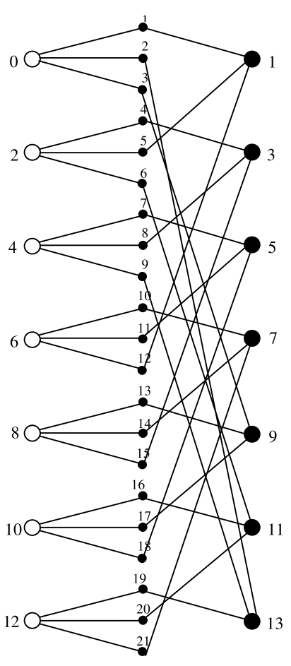
We introduce a set of (variable) vertices which correspond to the code symbols. Each of the (constraint) vertices on the right- and left-hand sides corresponds to one of 14 parity checks. The edges leaving one constraint vertex correspond to a codeword of the constituent block code of rate . The parity-check matrix of the corresponding graph-based code with binary constituent block codes is
| (1) |
where the parity-check matrix of size has the form
where is a size parity-check matrix of the constituent block code, and is a size parity-check matrix which is the permutation of the columns of determined by the graph. Notice that in general by choosing and assigning constituent block codes of different rates to the same graph we can obtain graph-based codes of different rates. In general, since in an -partite, -uniform, -regular hypergraph the total number of parity checks is equal to , the code rate of the graph-based code is
| (2) |
with equality if and only if all parity-checks are linearly independent. If , then we get .
The simplest example of a Heawood graph-based code can be obtained by choosing as constituent block codes a single-parity-check code of rate . Then the parity-check matrix has the form
and the parity-check matrix of the graph-based code is
| (3) |
In this case the graph-based code coincides with the graph code since (3) is the incidence matrix of the Heawood graph. In [4] it is proved that the minimum distance of the bipartite graph-based code with single-parity-check constituent codes is , where is the girth of the corresponding graph. Notice that for the Tanner graph we have . The parity-check matrix (3) is a parity-check matrix. Taking into account that one check is linearly dependent on the other, we obtain a binary block code. Its minimum distance is .
Consider the hypergraph shown in Fig. 1. Its incidence matrix has the form
| (4) |
and is a parity-check matrix of a hypergraph-based code which coincides with the parity-check matrix of the hypergraph code. Each column represents a hyperedge and each row represents a vertex of this hypergraph. For example, the first four rows represent the vertices 1, 2, 3, and 4 (triangles), the next four rows he vertices 5, 6, 7, and 8 (rectangles), and the last four rows the vertices 9, 10, 11, and 12 (ovals). The first column represents the hyperedge which connects the vertices 1, 5, and 9, the second column the hyperedge connecting vertices 1, 6, and 10 etc. The rows of (4) are linearly dependent. By removing two parity checks we obtain a linear block code with the minimum distance , where is the (,)-girth of the hypergraph. The rate of this hypergraph code is , which satisfies inequality (2),
The Tanner version of this hypergraph is shown in Fig. 5.
For an -partite, -uniform, -regular hypergraph-based code with constituent block codes we have the following theorem.
Theorem 1
The minimum distance of a hypergraph-based code based on an -partite, -uniform, -regular hypergraph with (,)-girth and containing constituent block codes with minimum distance is
Proof. Any nonzero codeword in an -partite, -uniform, -regular hypergraph-based code always corresponds to a connected -subgraph or a set of disjoint connected subgraphs. These subgraphs are called active [14], [4]. All hyperedges and vertices in an active subgraph are also called active. The number of hyperedges in the shortest connected subgraph is equal to . Any nonzero symbol in a codeword corresponds to an active hyperedge in the graph. By using the arguments given above, we conclude that for any codeword ,
where is the Hamming weight of . Minimizing over completes the proof.
II-B Woven graph codes with constituent block codes
Now assume that the constituent code assigned to the hypergraph vertices is a binary linear block code determined by a parity-check matrix
| (5) |
where is a size matrix, is the set of all possible binary matrices of size .
Let denote such a binary constituent block code determined by the matrix (5). We call the corresponding hypergraph-based code with as constituent codes a woven graph code with constituent block codes.
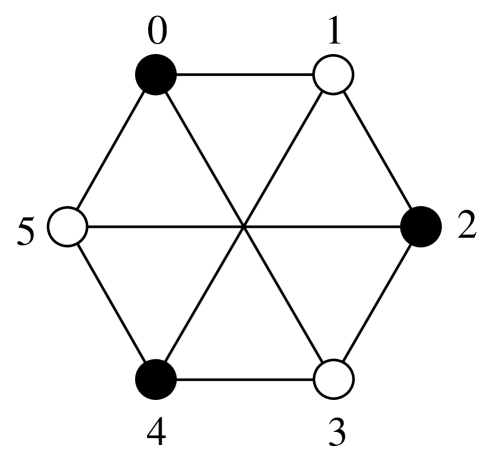
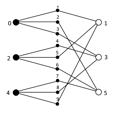
Consider an example of a woven graph code based on the bipartite graph with girth shown in Fig. 6. The Tanner version of this the so-called “utility” bipartite graph is shown in Fig. 7.
The incidence matrix of this graph is
| (6) |
We use a constituent () linear block code with determined by the parity-check matrix
By searching over all possible permutations of the matrices , , and we found the following parity-check matrix of the woven graph code with the best minimum distance
| (8) |
The matrix (8) describes a linear block code with .
Any codeword of the constituent block code can be represented as a sequence of blocks of length , that is, , where , . We define the minimum Hamming block distance between the codewords and of the constituent block code as
where , . Next we will prove the following theorem.
Theorem 2
The minimum distance of woven graph codes based on -partite, -uniform, -regular hypergraphs with (,)-girth and containing constituent block codes with minimum distance and minimum block distance can be lower-bounded by
Proof. Any nonzero codeword corresponds to an active connected subgraph or a set of disjoint connected subgraphs and the number of hyperedges in the shortest subgraph is . Any nonzero symbol in a codeword activates a hyperedge in the graph, that is, not less than constituent subcodes correspond to a codeword. Since at most hyperedges are connected with any hypergraph vertex then the number of active constituent subcodes can be lower-bounded by
Taking into account that any codeword of block weight greater than or equal to in the constituent block code has a weight at least equal to we obtain the following inequality
for any codeword and the proof is complete.
II-C Woven graph codes with constituent convolutional codes
Woven graph codes with constituent convolutional codes can be considered as a straightforward generalization of the woven graph code with constituent block codes. Assume that the code is chosen as a zero-tail terminated (ZT) convolutional code and consider a sequence of ZT convolutional codes with increasing . It is evident that when tends to infinity the constituent code can be chosen as a rate binary convolutional code with constraint length . Then the corresponding woven graph code has rate and its constraint length is at most .
Another description of woven graph codes with constituent convolutional codes follows from the representation of the constituent convolutional code in polynomial form. Let be a minimal encoding matrix [8] of a rate , memory convolutional code, given in polynomial form, that is,
| (9) |
where , , , are binary polynomials such that . The overall constraint length is . The binary information sequence is encoded as
where is a binary code sequence. Let denote a parity-check matrix for the same code,
| (10) |
where is the redundancy of the constituent code.
We denote by the field of binary Laurent series and regard a rate constituent convolutional code as a rate block code over the field of binary Laurent series encoded by . Then its codewords are elements of , which is the -dimensional vector space over the field of binary Laurent series [8].
The minimum Hamming block distance between the codewords and is defined [9] as
where is the Hamming (block) weight of .
Representing a convolutional code as a block code over the field of binary Laurent series we can obtain a woven graph code with constituent convolutional codes as a generalization of a graph-based code with binary constituent block codes. For example, a parity-check matrix of the rate Heawood’s graph-based code with constituent convolutional codes has the form
| (11) |
where and are short-hand for and , respectively, and is a parity-check matrix of the rate constituent convolutional code and is one of six possible permutations of .
Exploiting the above definitions we can interpret this bipartite woven graph-based code with constituent convolutional codes as follows. The left column of vertices in Fig. 4 represents parity checks each of which determines one of constituent fixed and identical convolutional codes and their branches represent the elements , even, , . Similarly, the right column of vertices represents same convolutional codes and their branches represent the elements , odd, , , where the set is a random permutation of the set determined by the graph.
We can also regard the left constituent convolutional codes as a warp with threads. Each of the right constituent convolutional codes are tacked on of the threads in the warp such that each thread of the warp is tacked on exactly once. Thus, our construction is a special case of a woven code [17] and we call this graph-based code a woven graph code.
Theorem 3
The free distance of a woven graph code based on an -partite, -uniform, -regular hypergraph with the (,)-girth and containing constituent convolutional codes with free distance and minimum block distance can be lower-bounded by
Proof. Since woven graph codes with constituent convolutional codes can be considered as a generalization of woven graph codes with constituent block codes, the theorem follows from Theorem 2 when tends to infinity.
For a woven graph code based on a bipartite graph with girth and containing constituent convolutional codes with minimum block distance and free distance by a straightforward generalization of the approach of [4] we obtain the following tighter bound on the free distance
| (12) |
III Asymptotic bounds on the minimum distance of woven graph codes
We will show that the ensemble of random woven graph codes based on random -partite, -uniform, -regular hypergraphs with a fixed degree and with a fixed number of vertices in each subgraph contains asymptotically good codes. In order to prove this we will modify the approach in [3].
III-A Woven graph codes with constituent block codes
First we consider the ensemble of random woven graph codes with rate constituent block codes determined by the edges of a random -partite, -uniform, -regular hypergraph corresponding to the time-varying random parity-check matrix
| (13) |
where , , is a block matrix of size (or a binary matrix of size ) and denotes a random permutation of the columns of ,
| (14) |
where , , denotes the random parity-check matrix (5) which determines the constituent block code and is the number of constituent codes in each subgraph.
Remark: In [3] a more restricted ensemble of random codes is studied in which all matrices are identical random matrices. In the proof of Theorem 1 we need that the syndrome components are independent random variables in the product probability space of random matrices and random permutations. The following simple example shows that this is not always the case if all matrices are identical.
Consider constituent block codes of block length with information symbols. This example is rather artificial since the rate of the constituent block code and therefore the rate of the graph-based code with is . In this case the parity-check matrix of the code has the form
where is a random permutation of elements. First assume that all matrices are identical, that is, . There are only 8 equiprobable elements in the product space, namely,
For any vector of weight 1 we have the following set of random equiprobable syndromes:
Therefore,
If and are both random and independent this probability is equal to 1/4.
Although this remark contradicts the proof of Theorem 3 in [3], there exists another (combinatorial) way to prove the same statement for identical [16].
Next we prove the following theorem.
Theorem 4
(Varshamov-Gilbert lower bound) For any , some , some integer and for all in the random ensemble of length woven graph codes with binary block constituent codes of rate there exist codes of rate such that their relative minimum distance satisfies the inequalities
| (19) |
where is a root of the equation
and is the solution of , and denotes the binary entropy function.
Proof. Let be the Hamming weight of the codeword of the random binary woven graph code . We are going to find a parameter such that the probability tends to 0 for all . We can rewrite as
| (20) |
where and denotes the number of nonzero constituent codewords in the th subgraph corresponding to the codeword of weight .
In the ensemble of random parity-check matrices , , of size the probability that a nonzero vector is a codeword of the corresponding constituent random binary code is equal to since the syndromes of the constituent codes are equiprobable sequences of length . Taking into account that in the th subgraph we have nonzero constituent codewords the probability can be upper-bounded by
| (21) |
In order to estimate the probability we prove the following lemma.
Lemma 1
For the ensemble of binary woven graph codes with constituent block codes described in Theorem 19, the probability that a codeword of weight contains nonzero constituent codewords in the subgraphs can be upper-bounded by
| (22) |
Proof. Taking into account that in the th subgraph the number of nonzero component codewords is equal to and that the subgraphs are random and independent we can rewrite the probability as
The probability can be upper-bounded as
where . The cardinality of can be upper-bounded as
| (23) |
where the sum is upper-bounded by the maximal term times the number of terms . ∎
Notice that in the above derivations we ignored the fact that can be noninteger since we consider the asymptotic behaviour of (20).
It follows from Lemma 1 that
| (24) |
Consider the asymptotic behaviour of (20) when tends to infinity. Introduce the notations and and the function
After simple derivations we obtain
| (25) |
where is the rate of binary woven graph code. Maximizing (25) over gives
Inserting and into (25) we obtain
| (26) |
which coincides with (9) and (10) in [3] for , that is, if the graph is bipartite.
For any and from , it follows that there exist codes of rate with relative minimum distance . Let denote the solution of the equation
| (27) |
for and let be the solution of . Solving (27) for and we obtain that there exist woven graph codes of rate with the relative minimum distance satisfying the inequalities:
| (28) |
∎
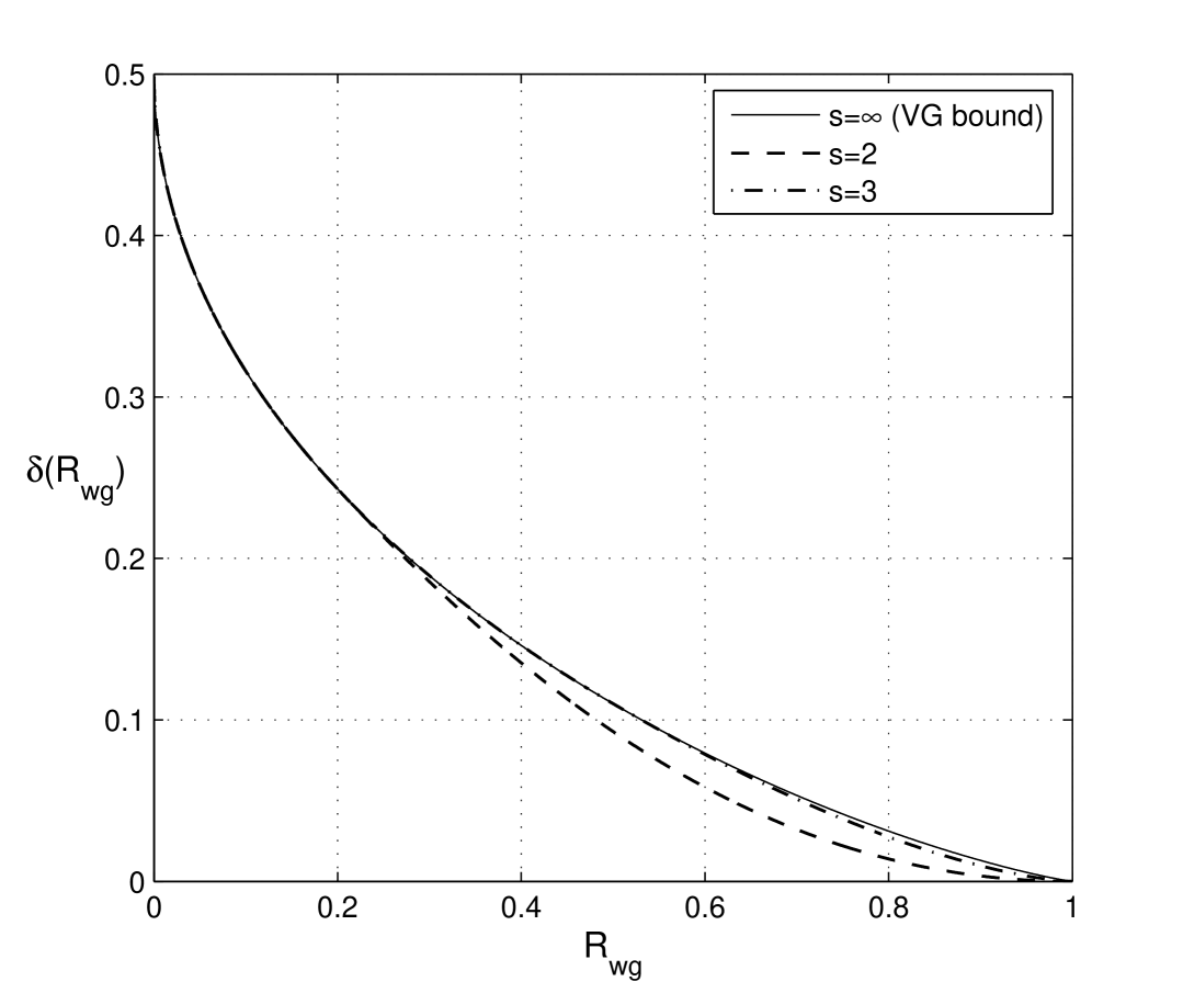
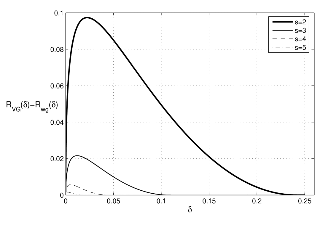
In Fig. 8 the lower bound (19) on the relative minimum distance for the ensemble of binary woven graph codes with block constituent codes as a function of the code rate is shown. It is easy to see that when grows the ensemble of binary woven graph codes contains codes meeting the VG bound for almost all rates . Fig. 9 demonstrates the gap between the VG bound and the code rate as a function of the relative minimum distance for different values of . It follows from Fig. 9 that for the difference in code rate compared to the VG bound is negligible.
III-B Asymptotic bound on the free distance of woven graph codes with constituent convolutional codes
Consider a ZT convolutional woven graph code with constituent ZT convolutional codes of rate . The length of a ZT woven graph codeword in -tuples is equal to where is the number of -tuples influenced by information symbols and is the memory of the woven graph code of rate . Denote by the free distance of the corresponding woven graph code.
Now we can prove the following
Theorem 5
(Costello lower bound) For any , some , some integer , and for all in the random ensemble of rate woven graph codes over -partite, -uniform, -regular hypergraphs with constituent convolutional codes of rate there exists a code with memory such that its relative free distance satisfies the Costello lower bound [8],
| (29) |
Proof: Analogously to the derivations in the proof of Theorem 4 let where denotes the number of nonzero constituent codewords in the th subgraph corresponding to the codeword of weight , . In order to evaluate the number of nonzero constituent codewords among the constituent codewords, notice that the set of such codewords is a union of sets of nonzero constituent codewords belonging to each of the subgraphs. The cardinality of the union is at least . Therefore the all-zero “tail” required to force the encoder into the zero state has length at least . The total number of redundant symbols consists of two parts: the number of parity-check symbols for the nonzero constituent codewords in the subgraphs and at least redundant symbols required for zero-tail terminating of the woven graph code. Thus, formula (21) can be rewritten as
| (30) |
The statement of the Lemma 22 is changed in a following way
| (31) |
Instead of (24) we now have
| (32) | |||||
IV Example
We start with considering a graph code determined by the parity-check matrix (3). As mentioned before, the matrix (3) can be considered as a parity-check matrix. Since the parity checks defined by the graph are linearly dependent (the sum of the rows of (3) is equal to zero) it turned out that by ignoring one parity check we obtain a parity-check matrix of a linear block code. For simplicity we consider the rate code that is obtained by ignoring the eighth information symbol which yields a subcode of this code.
It is easy to see that renumbering the graph vertices by adding to each vertex number some fixed number modulo the total number of vertices preserves both the incidence and adjacency matrices of the graph. For example, in Fig. 3, by adding 2 modulo 14 we will get exactly the same graph. When we have a similar property for linear codes we call such codes quasi-cyclic codes and these block codes can be described as tailbiting (TB) convolutional codes. Renumbering the vertices corresponds to permuting the rows of (3). By row permutations, (3) can be reduced to the form
| (37) |
It follows from (37) that the graph shown in Fig. 3 corresponds to a TB code with a parent convolutional code determined by the parity-check matrix
| (38) |
It means that this code is “tail-bitten” at the 7th level of the trellis diagram. A corresponding polynomial generator matrix of the parent convolutional code has the form
| (39) |
The minimum distance of the TB code is equal to the graph girth, that is, .
Notice that many regular bipartite graphs look very similar to the Heawood graph in the sense that by manipulating the incidence (parity-check) matrices and truncating lengths we can obtain infinite families of graphs. Some properties of these graphs can be easily predicted from the properties of the corresponding parent convolutional codes.
Consider the parity-check matrix (11) of the woven graph code based on the Heawood bipartite graph with constituent convolutional codes of rate . This woven graph code has the rate .
Let the rate constituent convolutional code of memory and overall constraint length with be given by the generator matrix
| (40) |
A corresponding parity-check matrix is
| (41) |
Notice that the constituent code considered as a block code over represents a block code with the minimum distance .
By using the product-type lower bound (12) we obtain
On the other hand, it was verified by computer search that any codeword of the woven graph code determined by (11) consists of at least three nonzero codewords of the component code described by (41). Moreover, it was found by computer search that each of these nonzero codewords of has the minimum block weight . Note that the codewords of the block code over with block weight corresponds to the codewords of the convolutional code belonging to its subcodes of rate . These three subcodes have generator matrices
where , , and .
The minimum free distance over all these subcodes of rate is equal to 8. Taking into account that all other codewords of the woven graph code contain at least four nonzero codewords of of block weight we obtain an improved lower bound on the free distance of the woven graph code as .
In order to obtain an upper bound on the free distance of the woven graph code we consider the parity-check matrix (11) in more detail. It also describes a quasi-cyclic code and can by row permutations be reduced to a parity-check matrix of a two-dimensional code, a TB (block) code in one dimension and a convolutional code in the other,
| (42) |
A parity-check matrix of the parent convolutional code for the TB code (42) given in symbolic form is
| (43) |
where and are formal variables. The matrix (43) can be considered as a parity-check matrix of a two-dimensional convolutional code. The variable corresponds to the parent convolutional code of the Heawood graph code (38), the variable is used for the constituent convolutional code (41).
A generator matrix of the two-dimensional convolutional code with the parity-check matrix (43) has the form
| (44) |
where , , , , , and .
The generator matrix (44) tail-bitten over variable at length yields the generator matrix of the code (42),
| (45) |
where is short-hand for .
Notice that any of the six permutations of the columns , generates a woven graph code. The permutation , , and describes the woven graph code with the largest free distance. The overall constraint length of this generator matrix is equal to 70 but the matrix is not in minimal form. A minimal-basic generator matrix [8] has the overall constraint length equal to 64 and differs from (45) by one row which can replace any of the rows of and has the form
where
where and .
The matrix (45) is a generator matrix of a convolutional code of rate . By applying the BEAST algorithm [19] to the minimal-basic generator matrices corresponding to the different permutations of the columns , we obtained the free distance and a few spectrum coefficients of the corresponding woven graph codes. The parameters of the best obtained woven graph codes are presented in Table 1.
V Encoding
Generally speaking, encoding of graph-based block codes has complexity , where is the blocklength. This technique implies that we find a generator matrix corresponding to the given parity-check matrix and then multiply the information sequence by the obtained generator matrix. However, we showed by examples that some regular graph codes as well as woven graph codes are quasi-cyclic codes and thereby they can be interpreted as TB codes. For this class of codes the complexity of the encoding is proportional to the constraint length of the parent convolutional code.
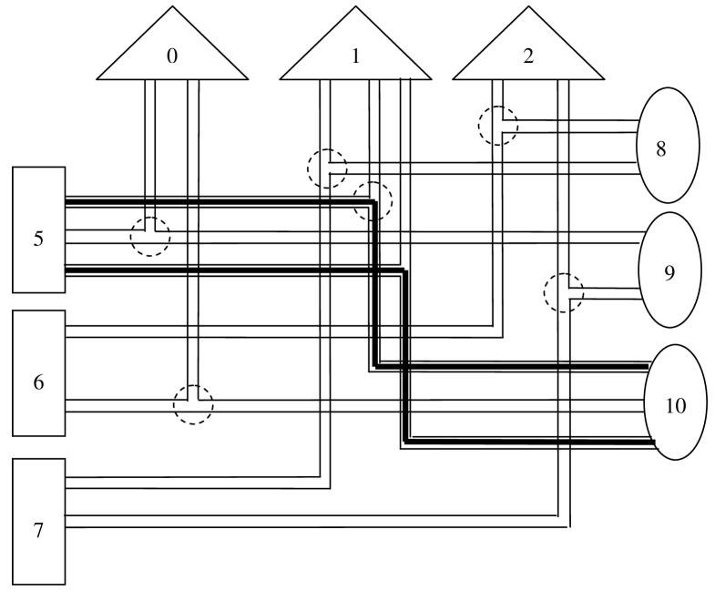
In this section we are going to illustrate by an example an encoder of a woven graph code with constituent convolutional codes having encoding complexity proportional to the overall constraint length of the corresponding woven graph code .
Consider again the woven graph code in our example. It is based on the Heawood graph and uses constituent convolutional codes of rate and overall constraint length . Taking into account the representation (45) of the woven graph code as a rate two-dimensional code, a TB (block) code in one dimension and a convolutional code in the other, we can draw its encoder as shown in Fig. 10.
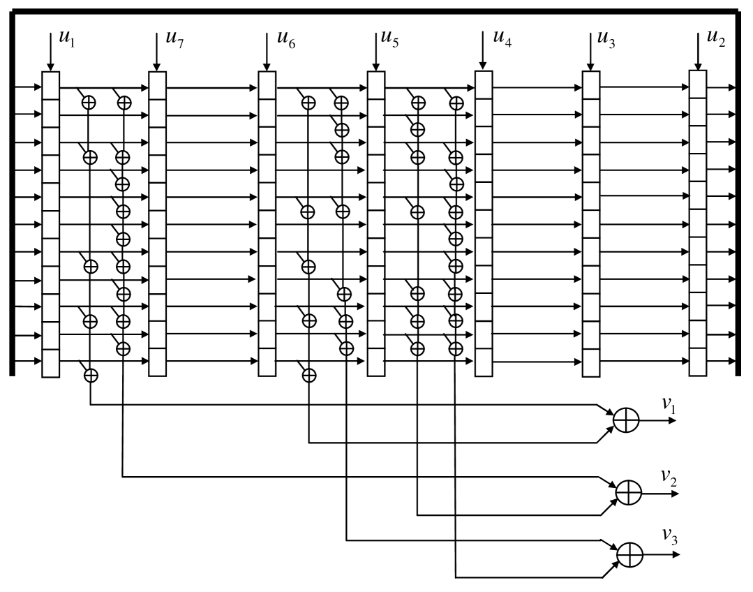
The input symbols enter the encoder once per each cycle of duration seven time instants. At each time moment the contents of each register is rewritten into the next (modulo seven) register and the three output symbols are generated. In other words, each of the registers corresponding to the constituent code can be considered as an enlarged delay element of the encoder of the “TB-dimension” code determined by the graph. The sequence determines a transition between the states of this encoder. After a cycle of seven time instants we return to the starting state of the enlarged encoder and a TB-codeword (or a word from one of its cosets) of length 21 has been generated. Then the following seven input symbols enter and after seven time instants another word of length 21 has been generated, etc.
VI Conclusion
The asymptotic behavior of the woven graph codes with block as well as with convolutional constituent codes has been studied. It was shown that in the random ensemble of such codes based on -partite, -uniform, -regular hypergraphs we can find a value such that for any code rate there exist codes meeting the VG and the Costello lower bound on the minimum distance and free distance, respectively. Product-type lower bounds on the minimum distance of graph-based and woven graph codes have been derived. Example of a rate woven graph code with free distance above the product bound is presented. It is shown, by an example, that woven graph codes can be encoded with a complexity proportional to the constraint length of the constituent convolutional code.
Acknowledgment
This work was supported in part by the Royal Swedish Academy of Sciences in cooperation with the Russian Academy of Sciences and in part by the Swedish Research Council under Grant 621-2007-6281.
References
- [1] R. G. Gallager, Low-density Parity-Check Codes, Cambridge, MA: MIT Press, 1963.
- [2] C. Berrou, A. Glavieux, and P. Thitimajshima, “Near Shannon limit error-correcting coding and decoding: Turbo codes,” in Proc. IEEE Int. Conf. Commun. (ICC), Geneva, Switzerland, pp. 1064–1070, 1993.
- [3] A. Barg and G. Zemor, “Distance properties of expander codes,” IEEE Trans. Inf. Theory, vol. 52, no.1, pp. 78–90, Jan. 2006.
- [4] X.-Y. Hu and M. F. Fossorier “On the computation of the minimum distance of low-density parity-check codes,” Int. Conference on Communications (ICC’04), Paris, June 2004.
- [5] G. Schmidt, V. V. Zyablov, and M. Bossert, “On expander codes based on hypergraphs,” ISIT 2003, Yokohama, Japan, June 29–July 4, 2003.
- [6] S. Hoory and Y. Bilu, “The codes from hypergraphs,” European Journal of Combinatorics vol. 25, Issue 3, pp. 339–354, April, 2004.
- [7] A. Barg, Private communication, May 2007.
- [8] R. Johannesson and K. Sh. Zigangirov, Fundamentals of Convolutional Coding, IEEE Press, Piscataway, NJ, 1999.
- [9] M. Bossert, C. Medina, and V. Sidorenko, “Encoding and distance estimation of product convolutional codes,” in Proc. IEEE Int. Symp. Information Theory (ISIT’05), Adelaide, Australia, Sept. 4-9, pp. 1063–1067, 2005.
- [10] J. A. Bondy and U. S. R. Murty, Graph theory with Applications, N.Y.: North Holland, pp. 236 and 244, 1976.
- [11] F. Harary, Graph theory, Reading, MA.:Addison-Wesley, p. 173, 1994.
- [12] G. Solomon and H. C. A. van Tilborg, “A connection between block and convolutional codes,” SIAM J. Appl. Math., vol. 37, pp. 358–369, 1979.
- [13] J. H. Ma and J. K. Wolf, “On tail-biting convolutional codes,” IEEE Trans. Commun., vol. COM-34, pp. 104–111, 1986.
- [14] R. M. Tanner, “Minimum-distance bounds by graph analysis,” IEEE Trans. Inf. Theory, vol. 47, no. 2, pp. 808–820, Feb. 2001.
- [15] R. M. Tanner, “A Recursive Approach to Low Complexity Codes,” IEEE Trans. Inf. Theory, vol. 27, no. 5, pp. 533–547, Sep. 1981.
- [16] L. Bassalygo, private communication, May 2007.
- [17] S. Hst, R. Johannesson, and V. V. Zyablov, “Woven convolutional codes I: Encoder properties,” IEEE Trans. Inf. Theory, vol. 48, no. 1, pp. 149–161, Jan. 2002.
- [18] R. M. Tanner, D. Sridhara, A. Sridharan, T. E. Fuja, and D. J. Costello, Jr., “LDPC Block and Convolutional Codes Based on Circulant Matrices,” IEEE Trans. Inf. Theory, vol. 50, no. 12, pp. 2966–2984, Dec. 2004.
- [19] I. E. Bocharova, M. Handlery, R. Johannesson, and B.D. Kudryashov, “A BEAST for prowling in trees,” IEEE Trans. Inf. Theory, vol. 50, no. 6, pp. 1295–1302, June 2004.
- [20] I. E. Bocharova, B. D. Kudryasov, R. Johannesson, and P. Stahl, “Tailbiting codes: bounds and search results,” IEEE Trans. Inf. Theory, vol. 48, no. 1, pp. 137–148, Jan. 2002.