33email: {sven.weinzierl, sandra.zilker, martin.matzner}@fau.de
33email: {jens.brunk, becker}@ercis.uni-muenster.de
33email: kate.revoredo@wu.ac.at
XNAP: Making LSTM-based Next Activity Predictions Explainable by Using LRP
Abstract
Predictive business process monitoring (PBPM) is a class of techniques designed to predict behaviour, such as next activities, in running traces. PBPM techniques aim to improve process performance by providing predictions to process analysts, supporting them in their decision making. However, the PBPM techniques’ limited predictive quality was considered as the essential obstacle for establishing such techniques in practice. With the use of deep neural networks (DNNs), the techniques’ predictive quality could be improved for tasks like the next activity prediction. While DNNs achieve a promising predictive quality, they still lack comprehensibility due to their hierarchical approach of learning representations. Nevertheless, process analysts need to comprehend the cause of a prediction to identify intervention mechanisms that might affect the decision making to secure process performance. In this paper, we propose XNAP, the first explainable, DNN-based PBPM technique for the next activity prediction. XNAP integrates a layer-wise relevance propagation method from the field of explainable artificial intelligence to make predictions of a long short-term memory DNN explainable by providing relevance values for activities. We show the benefit of our approach through two real-life event logs.
Keywords:
Predictive business process monitoring, explainable artificial intelligence, layer-wise relevance propagation, deep neural networks.1 Introduction
Predictive business process monitoring (PBPM) [14] emerged in the field of business process management (BPM) to improve the performance of operational business processes [5, 20]. PBPM is a class of techniques designed to predict behaviour, such as next activities, in running traces. PBPM techniques aim to improve process performance by providing predictions to process analysts, supporting them in their decision making. Predictions may reveal inefficiencies, risks and mistakes in traces supporting process analysts on their decisions to mitigate the issues [7]. Typically, PBPM techniques use predictive models, that are extracted from historical event log data. Most of the current techniques apply “traditional” machine-learning (ML) algorithms to learn models, which produce predictions with a higher predictive quality [6]. The PBPM techniques’ limited predictive quality was considered as the essential obstacle for establishing such techniques in practice [26]. Therefore, a plethora of works has proposed approaches to further increase predictive quality [22]. By using deep neural networks (DNNs), the techniques’ predictive quality was improved for tasks like the next activity prediction [9].
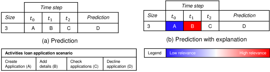
In practice, a process analyst’s choice to use a PBPM technique does not only depend on a PBPM technique’s predictive quality. Márquez-Chamorro et al. [15] state that the explainability of a PBPM technique’s predictions is also an important factor for using such a technique in practice. By providing an explanation of a prediction, the process analyst’s confidence in a PBPM technique improves and the process analyst may adopt the PBPM technique [17]. However, DNNs learn multiple representations to find the intricate structure in data, and therefore the cause of a prediction is difficult to retrieve [13]. Due to the lack of explainability, a process analysts cannot identify intervention mechanisms that might affect the decision making to secure the process performance. To address this issue, explainable artificial intelligence (XAI) has developed as a sub-field of artificial intelligence. XAI is a class of ML techniques that aims to enable humans to understand, trust and manage the advanced artificial “decision-supporters” by producing more explainable models, while maintaining a high level of predictive quality [10]. For instance, in a loan application process, the prediction of the next activity “Decline application” (cf. (a) in Fig. 1) produced by a model trained with a DNN can be insufficient for a process analyst to decide if this is a normal behaviour or some intervention is required to avoid an unnecessary refusal of the application. In contrast, the prediction with explanation (cf. (b) in Fig. 1) informs the process analyst that some important details are missing for approving the application because the activity “Add details” has a high relevance on the prediction of the next activity “Decline application”.
In this paper, we propose the explainable PBPM technique XNAP. XNAP integrates a layer-wise relevance propagation (LRP) method from XAI to make next activity predictions of a long short-term memory (LSTM) DNN explainable by providing relevance values for each activity in the course of a running trace. To the best of the authors’ knowledge, this work proposes the first approach to make LSTM-based next activity predictions explainable.
The paper is structured as follows. Sec. 2 introduces the required background. In Sec. 3, we present related work on explainable PBPM and reveal the research gap. Sec. 4 introduces the design of XNAP. In Sec. 5, the benefits of XNAP are demonstrated based on two real-life event logs. In Sec. 6 we provide a summary and point to future research directions.
2 Background
2.1 Preliminaries111Note definitions are inspired by the work of Taymouri et al. [23].
Definition 1 (Vector, Matrix, Tensor)
A vector is an array of numbers, in which the ith number is identified by . If each number of vector lies in and the vector contains numbers, then the vector lies in , and the vector ’s dimension is . A matrix is a two-dimensional array of numbers, where A tensor is an -dimensional array of numbers. If , then is a tensor of the third order with , where
Definition 2 (Event, Trace, Event Log)
An event is a tuple where is the case id, is the activity (event type) and is the timestamp. A trace is a non-empty sequence of events such that An event log is a set of traces. A trace can also be considered as a sequence of vectors, in which a vector contains all or a part of the information relating to an event, e.g. an event’s activity. Formally, where is a vector, and the superscript indicates the time-order upon which the events happened.
Definition 3 (Prefix and label)
Given a trace , a prefix of length , that is a non-empty sequence, is defined as with and a label (i.e. next activity) for a prefix of length is defined as . The above definition also holds for an input trace representing a sequence of vectors. For example, the tuple of all possible prefixes and the tuple of all possible labels for are and .
2.2 Layer-wise Relevance Propagation for LSTMs
LRP is a technique to explain predictions of DNNs in terms of input variables [3]. For a given input sequence , a trained DNN model and a calculated prediction , LRP reverse-propagates the prediction through the DNN model to assign a relevance value to each input variable of [1]. A relevance value indicates to which extent an input variable contributes to the prediction. Note is a DNN model, and is a target class for which we want to perform LRP. In this paper, is an LSTM model, i.e. a DNN model with an LSTM [11] layer as a hidden layer. The architecture of the “vanilla” LSTM (layer) is common in the PBPM literature for the task of predicting next activities [25]. For instance, an explanation of it can be found in the work of Evermann et al. [9].
To calculate the relevance values of the input variables, LRP performs two computational steps. First, it sets the relevance of an output layer neuron corresponding to the target class of interest to the value . It ignores the other output layer neurons and equivalently sets their relevance to zero. Second, it computes a relevance value for each intermediate lower-layer neuron depending on the neural connection type. A DNN’s layer can be described by one or more neural connections. In turns, the LRP procedure can be described layer-by-layer for different types of layers included in a DNN. Depending on the type of a neural connection, LRP defines heuristic propagation rules for attributing the relevance to lower-layer neurons given the relevance values of the upper-layer neurons [3].
In case of recurrent neural network layers, such as LSTM [11] layers, there are two types of neural connections: many-to-one weighted linear connections, and two-to-one multiplicative interactions [2]. Therefore, we restrict the definition of the LRP procedure to these types of connections. For weighted connections, let be an upper-layer neuron. Its value in the forward pass is computed as , while are the lower-layer neurons, and as well as are the connection weights and biases. Given each relevance of the upper-layer neurons , LRP computes the relevance of the lower-layer neurons . Initially, is set. The relevance distribution onto lower-layer neurons comprises two steps. First, by computing relevance messages going from upper-layer neurons to lower-layer neurons . The messages are computed as a fraction of the relevance accordingly to the following rule:
| (1) |
is the total number of lower-layer neurons connected to , is a stabiliser (small positive number, e.g. ) and is the sign of . Second, by summing up incoming messages for each lower-layer neuron to obtain relevance . is computed as . If the multiplicative factor is set to 1.0, the total relevance of all neurons in the same layer is conserved. If it is set to 0.0, the total relevance is absorbed by the biases.
For two-to-one multiplicative interactions between lower-layer neurons, let be an upper-layer neuron. Its value in the forward pass is computed as the multiplication of two lower-layer neuron values and , i.e. . In such multiplicative interactions, there is always one of two lower-layer neurons that represents a gate with a value range as the output of a sigmoid activation function. This neuron is called gate , whereas the remaining one is the source . Given such a configuration, and denoting by the relevance of the upper-layer neuron , the relevance can be redistributed onto lower-layer neurons by: and . With this reallocation rule, the gate neuron already decides in the forward pass how much of the information contained in the source neuron should be retained to make the overall classification decision.
3 Related Work on Explainable PBPM
In the past, PBPM research has mainly focus on improving the predictive quality of PBPM approaches to foster the transfer of these approaches into practice. In contrast, the PBPM approaches’ explainability was scarcely discussed although it can be equally important since missing explainability might limit the PBPM approaches’ applicability [15]. In the context of ML, XAI has already been considered in different approaches [4]. However, PBPM research has just recently started to focus on XAI. Researchers differentiate between two types of explainability. First, ante-hoc explainability provides transparency on different levels of the model itself; thus they are referred to as transparent models. This can be the complete model, single components or learning algorithms. Second, post-hoc explainability can be provided in the form of visualisations after the model was trained since they are extracted from the trained model [8].
Concerning ante-hoc explainability in PBPM, multiple approaches have been proposed for different prediction tasks. For example, Maggi et al. [14] propose a decision-tree-based, Breuker et al. [5] a probabilistic-based, Rehse et al. [18] a rule-based and Senderovic et al. [21] a regression-based approach.
In terms of post-hoc explainability, research has focused on model-agnostic approaches. These are techniques that can be added to any model in order to extract information from the prediction procedure [4]. In contrast, model-specific explanations are methods designed for certain models since they examine the internal model structures and parameters [8]. Fig. 2 depicts an overview of approaches for post-hoc explainability in PBPM. Verenich et al. [24] propose a two-step decomposition-based approach. Their goal is to predict the remaining time. First, they predict on an activity-level the remaining time. Next, these predictions are aggregated on a process-instance-level using flow analysis techniques. Sindhgatta et al. [22] provide both global and local explainability for XGBoost, this is for outcome and remaining time predictions. Global explanations are on a prediction-model-level. Therefore, the authors implemented permutation feature importance. On the contrary, Local explanations are on a trace-level, i.e. they describe the predictions regarding a trace. For this, the authors apply LIME [19]. This method perturbs the input, observes how predictions change and based on that, tries to provide explainability. Mehdiyev and Fettke [16] present an approach to make DNN-based process outcome predictions explainable. Thereby, they generate partial dependence plots (PDP) to provide causal explanations. Rehse et al. [18] create global and local explanations for outcome predictions. Based on a DL architecture with LSTM layers, they apply a connection weight approach to calculate the importance of features and therefore provide global explainability. For local explanations, the authors determine the contribution to the prediction outcome via learned rules and individual features.
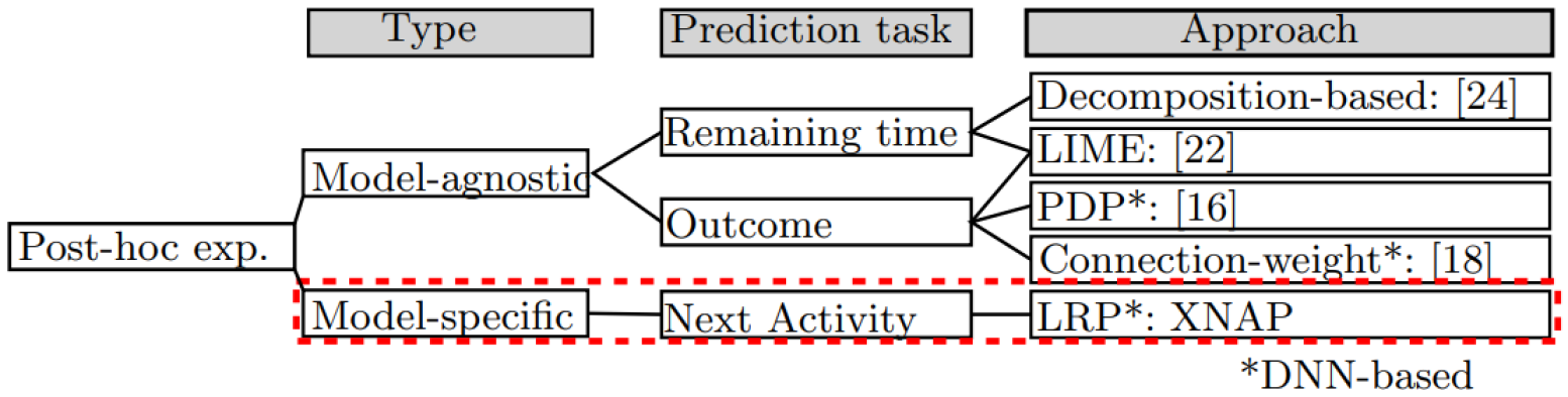
In comparison to those approaches, LRP is not part of the training phase and presumes a learned model. LRP peaks into the model to calculate relevance backwards from the prediction to the input. Thus, through the use of LRP, we contribute by providing the first model-specific post-hoc explanations of LSTM-based next activity predictions.
4 XNAP: Explainable Next Activity Prediction
XNAP is composed of an offline and an online component. In the offline component, a predictive model is learned from a historical event log by applying a Bi-LSTM DNN. In the online component, the learned model is used for producing next activity predictions in running traces. Given the next activity predictions and the learned predictive model, LRP determines relevance values for each activity of running traces.
4.1 Offline Component: Learning a Bi-LSTM model
The offline component receives as input an event log, pre-processes it, and outputs a Bi-LSTM model learned based on the pre-processed event log.
Pre-processing: The offline component’s pre-processing step transforms an event log into a data tensor and a label matrix (i.e. next activities). The procedure comprises four steps. First, we transform an event log into a matrix . is the event log’s size , whereas is the number of an event tuple’s elements. Note that we add an activity to the end of each sequence to predict their end. Second, we onehot-encode the string values of the activity attribute in because a Bi-LSTM requires a numerical input for calculating forward and backward propagations. After this step, we get the matrix , where is the number of different activity values in the event log . Third, we create prefixes and next activity labels. Thereby, a tuple of prefixes is created from by applying the function , whereas a tuple of labels is created from through the function . Lastly, we construct a third-order data tensor based on the prefix tuple as well as a label matrix based on the label tuple , where is the longest trace in the event log , i.e. . The remaining space for a sequence is padded with zeros, if .
Model learning: XNAP learns a Bi-LSTM model that maps the prefixes onto the next activity labels based on the data tensor and label matrix from the previous step. We use the Bi-LSTM architecture, an extension of “vanilla” LSTMs since Bi-LSTMs are forward and backward LSTMs that can exploit control-flow information from two directions of sequences. XNAP’s Bi-LSTM architecture comprises an input layer, a hidden layer, and an output layer. The input layer receives the data tensor and transfers it to the hidden layer. The hidden layer is a Bi-LSTM layer with a dimensionality of 100, i.e. the Bi-LSTM’s cell internal elements have a size of 100. We assign the activation function to the Bi-LSTM’s cell output. To prevent overfitting, we perform a random dropout of of input units along with their connections. The model connects the Bi-LSTM’s cell output to the neurons of a dense output layer. Its number of neurons corresponds to the number of the next activity classes. For learning weights and biases of the Bi-LSTM architecture, we apply the Nadam optimisation algorithm with a categorical cross-entropy loss and default values for parameters. Note that the loss is calculated based on the Bi-LSTM’s prediction and the next activity ground truth label stored in the label matrix . Additionally, we set the batch size to . Following Keskar et al. [12], gradients are updated after each 128th trace of the data tensor . Larger batch sizes tend to sharp minima and impair generalisation. The number of epochs (learning iterations) is set to , to ensure convergence of the loss function.
4.2 Online Component: Producing predictions with explanations
The online component receives as input a running trace, performs a pre-processing, creates a next activity prediction and concludes with the creation of a relevance value for each activity of the running trace regarding the prediction. The prediction is obtained by using the learned Bi-LSTM model from the offline component. Given the prediction, LRP determines the activity relevances by backwards passing the learned Bi-LSTM model.
Pre-processing: The online component’s pre-processing step transforms a running trace into a data tensor and a label matrix, as already described in the offline component’s pre-processing step. Note that we terminate the online phase if is since, for such traces, there is insufficient data to base prediction and relevance creation upon. Further, we assume that we have already observed all possible activities as well as the longest trace in the offline component. Thus, matrix and tensor lay in and . In the offline component, next activity labels are not known and based on the data tensor for a running trace a next activity is predicted.
Prediction creation: Given the data tensor from the previous step, the trained Bi-LSTM model from the offline component returns a probability distribution , containing the probability values of all activities. We retrieve the prediction from through , with .
Relevance creation: Lastly, we provide explainability of the prediction by applying LRP. For a next activity prediction , LRP determines a relevance value for each activity in the course of a running trace towards it by decomposing the prediction, from the output layer to the input layer, backwards through the model. Note the prediction was created in the previous step based on all activities of the running trace . In doing that, we apply the LRP approach proposed by Arras et al. [2] that is designed for LSTMs. As mentioned in Sec. 2, a layer of a DNN can be described by one or more neural connections. Depending on the layer’s type, LRP defines rules for attributing the relevance to lower-layer neurons given the relevance values of the upper-layer neurons. After backwards passing the model by considering conversation rules of different layers, LRP returns a relevance value for each onehot-encoded input activity of the data tensor . Finally, to visualise the relevance values, e.g. by a heatmap, positive relevance values are rescaled to the range and negative ones to the range .
5 Results
5.1 Event logs
We demonstrate the benefit of XNAP with two real-life event logs that are detailed in Table 1.
| Event log | #instances |
|
# events | # activities |
|
|
||||||
| helpdesk | 4,580 | 226 | 21,348 | 14 | [2;15;5;4] | [2;9;4;4] | ||||||
| bpi2019 | 24,938 | 3,299 | 104,172 | 31 | [1;167;4;4] | [1;11;4;4] | ||||||
| ∗[min; max; mean; median] | ||||||||||||
First, we use the helpdesk event log333https://data.mendeley.com/datasets/39bp3vv62t/1.. It contains data of a ticketing management process form a software company. Second, we make use of the bpi2019 event log444https://data.4tu.nl/repository/uuid:a7ce5c55-03a7-4583-b855-98b86e1a2b07.. It was provided by a coatings and paint company and depicts an order handling process. Here, we only consider sequences of max. events and extract a 10%-sample of the remaining sequences to lower computation effort.
5.2 Experimental Setup
LRP is a model-specific method that requires a trained model for calculating activity relevances to explain predictions. Therefore, we report the predictive quality of the trained models, and then demonstrate the activity relevances.
Predictive quality: To improve model generalisation, we randomly shuffle the traces of each event log. For that, we perform a process-instance-based sampling to consider process-instance-affiliation of event log entries. This is important since LSTMs map sequences depending on the temporal order of their elements. Afterwards, for each event log, we perform a ten-fold cross-validation. Thereby, in every iteration, an event log’s traces are split alternately into a 90%-training and 10%-test set. Additionally, we use 10% of the training set as a validation set. While we train the models with the remaining training set, we use the validation set to avoid overfitting by applying early stopping after ten epochs. Consequently, the model with the lowest validation loss is selected for testing. To measure predictive quality, we calculate the average weighted Accuracy (overall correctness of a model) and average weighted F1-Score (harmonic mean of Precision and Recall).
Explainability: To demonstrate the explainability of XNAP’s LRP, we pick the Bi-LSTM model with the highest F1-Score value and randomly select two traces from all traces of each event log. One of these traces has a size of five; the other one has a size of eight. We use traces of different sizes to investigate our approach’s robustness.
Technical details: We conducted all experiments on a workstation with 12 CPU cores, 128 GB RAM and a single GPU NVIDIA Quadro RXT6000. We implemented the experiments in Python 3.7 with the DL library Keras555https://keras.io. 2.2.4 and the TensorFlow666https://www.tensorflow.org. 1.14.1 backend. The source code can be found on Github777https://github.com/fau-is/xnap..
5.3 Predictive Quality
The Bi-LSTM model of XNAP predicts the next most likely activities for the helpdesk event log with an average (Avg) Accuracy and F1-Score of 84% and 79.8% (cf. Table 2). For the bpi2019 event log, the model achieves an Avg Accuracy and F1-Score of 75.5% and 72.7%. For each event log, the standard deviation (SD) of the Accuracy and F1-Score values is between 1.0% and 1.5%.
| Event log | Metric | 1 | 2 | 3 | 4 | 5 | 6 | 7 | 8 | 9 | 10 | Avg | Sd |
|---|---|---|---|---|---|---|---|---|---|---|---|---|---|
| helpdesk | Accuracy | 0.846 | 0.851 | 0.824 | 0.824 | 0.852 | 0.823 | 0.837 | 0.850 | 0.853 | 0.839 | 0.840 | 0.012 |
| F1-Score | 0.807 | 0.811 | 0.779 | 0.780 | 0.813 | 0.777 | 0.794 | 0.810 | 0.814 | 0.798 | 0.798 | 0.015 | |
| bpi2019 | Accuracy | 0.758 | 0.759 | 0.748 | 0.762 | 0.754 | 0.758 | 0.753 | 0.734 | 0.748 | 0.772 | 0.755 | 0.010 |
| F1-Score | 0.732 | 0.737 | 0.712 | 0.741 | 0.722 | 0.730 | 0.723 | 0.710 | 0.720 | 0.742 | 0.727 | 0.011 |
5.4 Explainability
We show the activity relevance values of XNAP’s LRP on the example of two traces per event log (cf. Fig. 3). The time steps (columns) represent the activities that are used as input. For each trace, we predict the next activity for different prefix lengths (rows). We start with a minimum of three and make one next activity prediction until the maximum length of the trace is reached (five and eight in our examples). The data-given ground truth is listed in the last column. We use a heatmap to indicate the relevance of the input activities to the prediction of the same row.
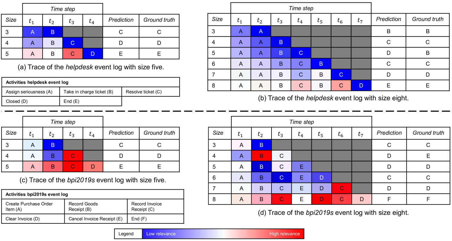
For example, in the traces (a) and (b), the activity “Resolve ticket” (C) has a high relevance on predicting the next activity “End (E)”. With that, a process analyst knows that the trace will end since the ticket was resolved. Another example is in the traces (c) and (d), where the activity “Record Invoice Receipt (C)” has a high relevance on predicting the next activity “Clear Invoice (D)”. Thus, a process analyst knows that the invoice can be cleared in the next step because the invoice receipt was recorded.
6 Conclusion
Given the fact that DNNs achieve a promising predictive quality at the expense of explainability and based on our identified research gap, we argue that there is a crucial need for making LSTM-based next activity predictions explainable. We introduced XNAP, an explainable PBPM technique, that integrates an LRP method from the field of XAI to make a BI-LSTM’s next activity prediction explainable by providing a relevance value for each activity in the course of a running trace. We demonstrated the benefits of XNAP with two event logs. By analysing the results, we made three main observations. First, LRP is a model-specific XAI method; thus, the quality of the relevance scores depend strongly on the model’s predictive quality. Second, XNAP performs better for traces with a smaller size and a higher number of different activities. Third, XNAP computes the relevance values of activities in very few seconds. In contrast, model-agnostic approaches, e.g. PDP [16], need more computation time.
In future work, we plan to validate our observations with further event logs. Additionally, we will conduct an empirical study to evaluate the usefulness of XNAP. We also plan on hosting a workshop with process analysts to better understand how a prediction’s explainability contributes to the adoption of a PBPM system. Moreover, we plan to adapt the propagation rules of XNAP’s LRP also to determine relevance values of context attributes. Another avenue for future research is to compare the explanation capability of a model-specific method like LRP to a model-agnostic method like LIME for, e.g. the DNN-based next activity prediction. Finally, XNAP’s explanations, which are rather simple, might not capture an LSTM model’s complexity. Therefore, future research should investigate new types of explanations that better represent this high complexity.
Acknowledgments
This project is funded by the German Federal Ministry of Education and Research (BMBF) within the framework programme Software Campus under the number 01IS17045. The fourth author received a grand from Österreichische Akademie der Wissenschaften.
References
- [1] Arras, L., Arjona-Medina, J., Widrich, M., Montavon, G., Gillhofer, M., Müller, K.R., Hochreiter, S., Samek, W.: Explaining and interpreting LSTMs. In: Explainable AI: Interpreting, explaining and visualizing deep learning, pp. 211–238. Springer (2019)
- [2] Arras, L., Montavon, G., Müller, K.R., Samek, W.: Explaining recurrent neural network predictions in sentiment analysis. In: Proceedings of the 8th Workshop on Computational Approaches to Subjectivity, Sentiment and Social Media Analysis. pp. 159–168. ACL (2017)
- [3] Bach, S., Binder, A., Montavon, G., Klauschen, F., Müller, K.R., Samek, W.: On pixel-wise explanations for non-linear classifier decisions by layer-wise relevance propagation. PloS one 10(7), e0130140 (2015)
- [4] Barredo Arrieta, A., Díaz-Rodríguez, N., Del Ser, J., Bennetot, A., Tabik, S., Barbado, A., Garcia, S., Gil-Lopez, S., Molina, D., Benjamins, R., Chatila, R., Herrera, F.: Explainable artificial intelligence (XAI): Concepts, taxonomies, opportunities and challenges toward responsible AI. Information Fusion 58, 82–115 (2020)
- [5] Breuker, D., Matzner, M., Delfmann, P., Becker, J.: Comprehensible predictive models for business processes. MIS Quarterly 40(4), 1009–1034 (2016)
- [6] Di Francescomarino, C., Ghidini, C., Maggi, F., Milani, F.: Predictive process monitoring methods: Which one suits me best? In: Proceedings of the 16th International Conference on Business Process Management. pp. 462–479. Springer (2018)
- [7] Di Francescomarino, C., Ghidini, C., Maggi, F., Petrucci, G., Yeshchenko, A.: An eye into the future: Leveraging a-priori knowledge in predictive business process monitoring. In: Proceedings of the 15th International Conference on Business Process Management. pp. 252–268. Springer (2017)
- [8] Du, M., Liu, N., Hu, X.: Techniques for interpretable machine learning. Communications of the ACM 63(1), 68–77 (2019)
- [9] Evermann, J., Rehse, J.R., Fettke, P.: Predicting process behaviour using deep learning. Decision Support Systems 100, 129–140 (2017)
- [10] Gunning, D.: Explainable artificial intelligence (XAI). Defense Advanced Research Projects Agency 2 (2017)
- [11] Hochreiter, S., Schmidhuber, J.: Long short-term memory. Neural Computation 9(8), 1735–1780 (1997)
- [12] Keskar, N.S., Mudigere, D., Nocedal, J., Smelyanskiy, M., Tang, P.T.P.: On large-batch training for deep learning: Generalization gap and sharp minima. In: Proceedings of the 5th International Conference on Learning Representations. pp. 1–16. openreview.net (2017)
- [13] LeCun, Y., Bengio, Y., Hinton, G.: Deep learning. Nature 521(7553), 436 (2015)
- [14] Maggi, F., Di Francescomarino, C., Dumas, M., Ghidini, C.: Predictive monitoring of business processes. In: Proceedings of the 26th International Conference on Advanced Information Systems Engineering. pp. 457–472. Springer (2014)
- [15] Márquez-Chamorro, A., Resinas, M., Ruiz-Cortás, A.: Predictive monitoring of business processes: a survey. Transactions on Services Computing pp. 1–18 (2017)
- [16] Mehdiyev, N., Fettke, P.: Prescriptive process analytics with deep learning and explainable artificial intelligence. In: Proceedings of the 28th European Conference on Information Systems. AISeL (2020)
- [17] Nunes, I., Jannach, D.: A systematic review and taxonomy of explanations in decision support and recommender systems. User Modeling and User-Adapted Interaction 27(3-5), 393–444 (2017)
- [18] Rehse, J.R., Mehdiyev, N., Fettke, P.: Towards explainable process predictions for industry 4.0 in the DFKI-Smart-Lego-Factory. Künstliche Intelligenz 33(2), 181–187 (2019)
- [19] Ribeiro, M.T., Singh, S., Guestrin, C.: “Why should I trust you?” Explaining the predictions of any classifier. In: Proceedings of the 22nd International Conference on Knowledge Discovery and Data Mining. pp. 1135–1144 (2016)
- [20] Schwegmann, B., Matzner, M., Janiesch, C.: precep: Facilitating predictive event-driven process analytics. In: Proceedings of the 8th International Conference on Design Science Research in Information Systems. pp. 448–455. Springer (2013)
- [21] Senderovich, A., Di Francescomarino, C., Ghidini, C., Jorbina, K., Maggi, F.M.: Intra and inter-case features in predictive process monitoring: A tale of two dimensions. In: Proceedings of the 15th International Conference on Business Process Management. pp. 306–323. Springer (2017)
- [22] Sindhgatta, R., Ouyang, C., Moreira, C., Liao, Y.: Interpreting predictive process monitoring benchmarks. arXiv:1912.10558 (2019)
- [23] Taymouri, F., La Rosa, M., Erfani, S., Bozorgi, Z.D., Verenich, I.: Predictive business process monitoring via generative adversarial nets: The case of next event prediction. arXiv:2003.11268 (2020)
- [24] Verenich, I., Dumas, M., La Rosa, M., Nguyen, H.: Predicting process performance: A white-box approach based on process models. Journal of Software: Evolution and Process 31(6), e2170 (2019)
- [25] Weinzierl, S., Zilker, S., Brunk, J., Revoredo, K., Nguyen, A., Matzner, M., Becker, J., Eskofier, B.: An empirical comparison of deep-neural-network architectures for next activity prediction using context-enriched process event logs. arXiv:2005.01194 (2020)
- [26] Weinzierl, S., Revoredo, K.C., Matzner, M.: Predictive business process monitoring with context information from documents. In: Proceedings of the 27th European Conference on Information Systems. pp. 1–10. AISeL (2019)